Distribution Function of Dark Matter with Constant Anisotropy

Abstract

N-body simulations of dark matter halos show that the density is cusped near the center of the halo. The density profile behaves as $r^{-\gamma}$ in the inner parts, where $\gamma\simeq 1$ for the NFW model and $\gamma\simeq 1.5$ for the Moore’s model, but in the outer parts, both models agree with each other in the asymptotic behavior of the density profile. The simulations also show the information about anisotropy parameter $\beta(r)$ of velocity distribution. $\beta\approx 0$ in the inner part and $\beta\approx 0.5$ (radially anisotropic) in the outer part of the halo. We provide some distribution functions $F(E,L)$ with the constant anisotropy parameter $\beta$ for the two spherical models of dark matter halos: a new generalized NFW model and a generalized Moore model. There are two parameters $\alpha$ and $\epsilon$ for those two generalized models to determine the asymptotic behavior of the density profile. In this paper, we concentrate on the situation of $\beta(r)=1/2$ from the viewpoint of the simulation.

Managing Editor

1 Introduction

The dark matter halo can be considered as the collisionless self-gravitational system which is described by the Vlasov equation and the Poisson equation. Apart from observations, there are mainly two approaches to the study of dark matter halos: (1) numerical simulations and (2) analytic or semi-analytic method.

Nowadays, N-body simulations become more and more important in the study of dark matter halos. Those simulations provide density profile and other properties of dark matter halos such as anisotropy of velocity distribution. A ’universal’ density profile of dark matter halo was proposed by Navarro, Frenk, $\&$ White (hereafter NFW)[1, 2]. The NFW profile is shown as $\rho\propto 1/((r/r_{s})(1+r/r_{s})^{2})$, where $r_{s}$ is a characteristic radius. We can find directly from the NFW profile that $\rho\propto r^{-1}$ near the center and $\rho\propto r^{-3}$ in the outer parts. Some simulations’ results exhibit different inner logarithmic slopes from NFW’s but deviate not so much from the latter’s in the outer parts of the halo. In the inner parts of the halo, Moore’s profile[3] behaves as $\rho\propto r^{-1.5}$. Jing and Suto’s profile[4] behaves as $\rho\propto r^{-\gamma}$ in the inner part, where the density logarithmic slopes $\gamma\simeq 1.1\sim 1.5$ with different merger histories and different total mass of the halos. Some other simulations concentrate on the outer slope of the dark matter density. For example, Avila-Reese et al. found that outer slopes $\gamma$ of some halos are larger than NFW’s outer slopes($\gamma=3$)[5]. What’s more, Hansen and Moore[6, 7] found that the density logarithmic slopes $\gamma$ is correlated with the velocity anisotropy which is parameterized as an anisotropy parameter $\beta$ and they provided the formula $\beta\approx 1-1.15(1-\gamma/6)$. So $\beta\approx 0$ in the inner part as $\gamma\approx 1$ and $\beta\approx 0.5$ in the outer part as $\gamma\approx 3$.

On the other hand, many authors try to construct the dynamical models of the stellar system and the dark matter halo analytically or semi-analytically. It is important to construct the dynamical models which have physical meaning, as for instance, these analytic or semi-analytic dynamical models can be used to generate the initial conditions of N-body simulations[20]. A stellar system or a dark matter halo is described by the distribution functions(DFs) F(x,v). Eddington (1916) showed how to determine the DF of a spherical symmetric stellar system with the isotropic velocity distribution[9], but it is difficult to calculate the distribution function in the anisotropic cases. A pioneer work on the anisotropic cases is called King-Michie model[10, 11] that comes from an approximate steady state solution of the Fokker-Planck equation. In the past few years, there has been great progress in the anisotropic cases. Dejonghe took a large step on finding anisotropic distribution function with using the augmented density $\rho(\psi,r)$[12, 13]. Some authors constructed the anisotropic models with constant anisotropy parameter[14]. For another kind of models called the Osipkov-Merritt models[15, 16, 17], the velocity dispersion tensor becomes isotropic near the center and becomes completely radial anisotropic in the outer part of the halo. Cuddeford[18] constructed the modified Osipkov-Merritt model which allows the velocity dispersion tensor to be an arbitrary anisotropy in the inner part of the halo but still completely radial anisotropy in the outer part and the composite Osipkov-Merritt model was constructed by Ciotti $\&$ Pellegrini[19]. Furthermore, Baes $\&$ Hese[20] constructed a dynamical model with seven parameters very recently to get a flexible anisotropy profile. Some authors built a model[21] to erase the cusp in the center of the halo.

To construct the dynamical models(or DFs) with flexible anisotropy behavior, some special potential-density pairs have been considered. For example, the Plummer model[13, 22], anisotropic Veltmann model[23], the Hernquist model[24, 25] and the $\gamma-$model[26, 27, 28, 29]. Some authors study this matter in other ways. Some assumed simple DFs at first and then solved the the potential and the density profiles[30, 31]. Widrow[32] provided the Osipkov-Merritt DFs and DEDs (differential energy distributions) for the NFW profile by the semi-analytic method.

Recently, Evans and An[14] have provided the DFs with constant anisotropy of the dark matter for two types of the density profiles. One is the generalized NFW profiles, $\rho\propto 1/(r(a+r)^{b-1})$, and the other is the Gamma model, $\rho\propto 1/(r^{\gamma}(a+r)^{4-\gamma})$. Both in these two models, asymptotic behaviors of density profiles are controlled by only one parameter. In this paper, we provide the DFs with constant anisotropy of the dark matter for more generalized density profiles in a semi-analytical way. Our generalized density profiles, with two parameters $\alpha$ and $\epsilon$, can cover many realistic profiles which come from simulations.

In Section 2 we review the basic knowledge needed for this paper and the main ideas of DF with constant anisotropy. Section 3 provides DFs of two models for dark matter halos: a new generalized NFW model and a generalized Moore model. We make the discussion and conclusion in Section 4.

2 Basic Properties

2.1 General formulae

For the spherically symmetric stellar system with the isotropic velocity field, a mass distribution function $F(E)$ describes this system very well. The mass density can be obtained from the distribution function[12],

$$\rho(\psi)=4\pi\int_{0}^{\psi}F(E)\sqrt{2(\psi-E)}dE\ ,$$ (1)

where the binding energy $E$ is defined as

$$E=\psi(r)-\tfrac{1}{2}\,v_{r}^{2}-\tfrac{1}{2}\,v_{T}^{2}\ ,$$ (2)

and $\psi(r)$ is the relative gravitational potential which can be obtained from the Poisson equation:

$$\frac{1}{r^{2}}\,\frac{d}{dr}\left(r^{2}\,\frac{d\psi}{dr}\right)=-4\pi G\rho(r)\ .$$ (3)

$v_{r}$ is the radial velocity and $v_{T}$ is the tangential velocity:

$$v_{T}=\sqrt{v_{\theta}^{2}+v_{\varphi}^{2}}\ .$$ (4)

Eddington[9] provided the inversion formula of the Eq. (1):

$$F(E)=\frac{1}{2\pi^{2}}D_{E}\int_{0}^{E}\frac{d\rho(\psi)}{d\psi}\frac{d\psi}{\sqrt{2(E-\psi)}}\ ,$$ (5)

where $D_{E}$ denotes the differentiation with respect to $E$.

The anisotropy parameter[8] mentioned in the Introduction is defined as:

$$\beta=1-\frac{\sigma_{T}^{2}}{2\sigma_{r}^{2}}\ ,$$ (6)

where $\sigma_{T}^{2}$ and $\sigma_{r}^{2}$ are the tangential and radial velocity dispersion. If $\beta<0$, $\sigma_{T}^{2}>2\sigma_{r}^{2}$ (tangentially anisotropic). If $0<\beta\leq 1$, $\sigma_{T}^{2}<2\sigma_{r}^{2}$ (radially anisotropic). Else If $\beta=0$, $\sigma_{T}^{2}=2\sigma_{r}^{2}$ (isotropic case). Specially, $\beta\rightarrow-\infty$ means that every particle is in a circular orbit and $\beta=1$ indicate that every particle is in a radial orbit.

The anisotropic case is different from the isotropic one as we should consider the modulus of the angular momentum vector[12] $L=rv_{T}$ and therefore now the distribution function of dark matter depends on two variables $E$ and $L$. Then, the mass density can be obtained from $F(E,L)$ by the double integration[12]

$$\rho(\psi,r)=2\pi\int_{0}^{\psi}dE\int_{0}^{2(\psi-E)}\frac{F(E,L)}{\sqrt{2(\psi-E)-v_{T}^{2}}}dv_{T}^{2}\ .$$ (7)

However, the inversion formula of the above equation is much more difficult to obtain than that in the isotropic case. Many works have been done for this problem just as mentioned in the Introduction.

2.2 Distribution function with constant anisotropy

There is a simple and widely used ansatz for $F(E,L)$ as below[12, 14, 18, 33, 34]:

$$F(E,L)=L^{-2\beta}f(E)\ .$$ (8)

The simulations indicate that the anisotropy parameter $\beta(r)$ varies radially , but for the DF above, $\beta(r)$ is constant. Although this simple ansatz is very attractive in the calculation of inversion formula of Eq. (7), the assumption of constant anisotropy parameter is not so ideal. Anyway, we can still use this valuable assumption which pave the way for the further work.

From Eq. (7) and Eq. (8) we can get $\rho$ from $F(E,L)$,

$$\rho(\psi,r)=r^{-2\beta}\,\frac{(2\pi)^{3/2}\Gamma(1-\beta)}{2^{\beta}\Gamma(3/2-\beta)}\int_{0}^{\psi}\!(\psi-E)^{1/2-\beta}f(E)\,dE\ .$$ (9)

The function $f(E)$ can be given from the inversion formula[14, 18, 33] of the above equation.

$$f(E)=\frac{2^{\beta}(2\pi)^{-3/2}}{\Gamma(1-\lambda)\Gamma(1-\beta)}\ \frac{d}{dE}\!\int_{0}^{E}\frac{d\psi}{(E-\psi)^{\lambda}}\frac{d^{n}h}{d\psi^{n}}\ ,$$ (10)

where $h(\psi)=r^{2\beta}\rho$ is expressed as a function of $\psi$, $n=\lfloor(3/2-\beta)\rfloor$ and $\lambda=3/2-\beta-n$ is the integer floor and the fractional part of $3/2-\beta$. The DED now can be expressed as [14, 18]

$$\frac{dM}{dE}=f(E)\,\frac{(2\pi)^{5/2}\Gamma(1-\beta)}{2^{\beta-1}\Gamma(3/2-\beta)}\int_{0}^{r_{E}}(\psi-E)^{1/2-\beta}r^{2(1-\beta)}dr\ ,$$ (11)

where $r_{E}$ is defined through $\psi(r_{E})=E$. It is clear that $r_{E}$ is the largest radius reachable by a particle with binding energy E.

The expressions of DFs and DEDs are relatively simple if $\beta$ is a half integer (i.e., $\beta=3/2,1/2,-1/2...$). Specifically, in the case of $\beta=1/2$, which is more suitable from the viewpoint of the simulation, the expressions of DF and DED further reduce to[14]

$$\begin{split}&F(E,L)=\frac{g(r_{E})}{2\pi^{2}L}\,,\qquad\frac{dM}{dE}=2\pi r_{E}^{2}g(r_{E}),\\ &g(r_{E})=\left.\frac{\rho+r(d\rho/dr)}{(d\psi/dr)}\right|_{r=r_{E}}.\end{split}$$ (12)

In this paper, we select $\beta=1/2$ for our models just as Ref. EA06 by the same token.

3 Dark Matter Halo Models

3.1 New generalized NFW profiles

Let us consider a family of density profiles with parameters $\alpha$ and $\epsilon$

$$\rho=C\frac{1}{(r/r_{s})^{\alpha}(1+r/r_{s})^{3+\epsilon-\alpha}}\ .$$ (13)

We set the characteristic radius $r_{s}=1$, the total mass $M_{tot}=1$ and the gravitational constant $G=1$ here, and then the density profiles reduce to

$$\rho=C\frac{1}{r^{\alpha}(1+r)^{3+\epsilon-\alpha}}\ ,$$ (14)

$$C=\frac{\Gamma(3-\alpha+\epsilon)}{4\pi\Gamma(3-\alpha)\Gamma(\epsilon)}\ .$$ (15)

With two parameters $\alpha<3$ and $\epsilon>0$ we can freely select the asymptotic behavior of the density profile both in the inner and outer part of the halo. For the cases of $0<\epsilon\ll 1$, the profile closes to the NFW profiles when $\alpha\rightarrow 1$ and is similar to the Moore or Jing & Suto’s profile if $\alpha=1.1\sim 1.5$. If $\epsilon=1$, the profile just reduces to the $\gamma$ model.

We can calculate the relative potential $\psi$ from the Poisson equation.

$$\begin{split}&\psi(r)=C\left[c_{0}-4\pi r^{-\alpha}\Gamma(-\alpha)\left(A_{1}(r)-2A_{2}(r)+A_{3}(r)\right)\right]\\ &\\ &A_{1}(r)=\ _{2}\tilde{F}_{1}[1-\alpha+\epsilon,\ -\alpha,\ 2-\alpha,\ -r]\\ &A_{2}(r)=\ _{2}\tilde{F}_{1}[2-\alpha+\epsilon,\ -\alpha,\ 2-\alpha,\ -r]\\ &A_{3}(r)=\ _{2}\tilde{F}_{1}[3-\alpha+\epsilon,\ -\alpha,\ 2-\alpha,\ -r]\end{split}$$ (16)

where $c_{0}$ is determined by the condition $\left.\psi(r)\right|_{r\rightarrow\infty}=0$. Note that $\Gamma(-\alpha)$ is singular when $\alpha=1,2$. We find that $\psi$ cannot satisfy the condition $\left.\psi(r)\right|_{r\rightarrow\infty}=0$ when $\alpha\rightarrow 2$, but there is no problem for $\alpha\rightarrow 1$. In this paper, we focus on the situation of $\alpha=1\sim 1.5$ from the viewpoint of the N-body simulation.

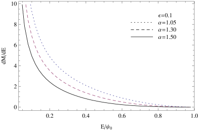
Figure 1: The energy part of the distribution function (left panel) and the differential energy distribution (right panel) of the New Generalized NFW model with the constant anisotropy parameter $\beta=1/2$ and $\epsilon=0.1$: dotted lines ($\alpha=1.05$, closes to the NFW model), dashed lines ($\alpha=1.30$), solid lines ($\alpha=1.50$, where the asymptotic behavior of density profile is similar to the Moore model).

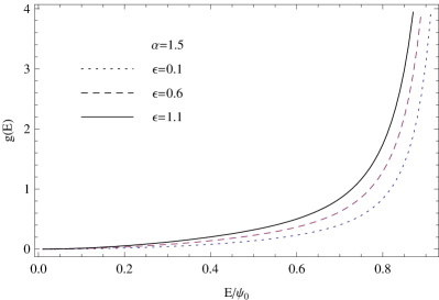
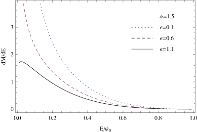
Figure 2: The energy part of the distribution function (left panel) and the differential energy distribution (right panel) of the New Generalized NFW model with the constant anisotropy parameter $\beta=1/2$ and $\alpha=1.5$: dotted lines ($\epsilon=0.1$, where the asymptotic behavior of density profile is similar to the Moore model), dashed lines ($\epsilon=0.6$), solid lines ($\epsilon=1.1$).

Now we can get $g(r_{E})$ from Eq. (12) and Eq. (16):

$$\begin{split}&g(r_{E})=\left.\frac{B_{1}(r)}{4\pi\alpha\Gamma(-\alpha)[B_{2}(r)A_{4}(r)+B_{3}(r)A_{5}(r)]}\right|_{r=r_{E}}\\ &\\ &B_{1}(r)=-(-2+\alpha-\epsilon)\ (-1+\alpha-\epsilon)\ [-1+\alpha+(2+\epsilon)r]\ r\ (1+r)^{-2+\alpha-\epsilon}\\ &B_{2}(r)=(2-\alpha)+(4+2\epsilon-3\alpha)r+[(2+\epsilon)(1+\epsilon)-\alpha(3+2\epsilon)]r^{2}\\ &B_{3}(r)=\alpha-2+(2\alpha\ -3-\epsilon)r\\ &A_{4}(r)=\ _{2}\tilde{F}_{1}[1-\alpha,\ 1-\alpha+\epsilon,\ 2-\alpha,\ -r]\\ &A_{5}(r)=\ _{2}\tilde{F}_{1}[-\alpha,\ 1-\alpha+\epsilon,\ 2-\alpha,\ -r]\end{split}$$ (17)

Note that $B_{1}(r)=0$ if $\alpha-\epsilon=1,2$. However, $g(r_{E})$ doesn’t approach zero when $\alpha-\epsilon\rightarrow 1,2$. We also find that $\alpha$ should be larger than $1$ as the distribution function should be positive. We couldn’t get the $r_{E}$ from $\psi(r_{E})=E$ analytically but can get the numerical solutions. $F(E,L)$ and $dM/dE$ are expressed as:

$$F(E,L)=\left.\frac{B_{1}(r)}{8\pi^{3}L\alpha\Gamma(-\alpha)[B_{2}(r)A_{4}(r)+B_{3}(r)A_{5}(r)]}\right|_{r=r_{E}}$$ (18)

$$\frac{dM}{dE}=\left.\frac{r^{2}\ B_{1}(r)}{2\alpha\Gamma(-\alpha)[B_{2}(r)A_{4}(r)+B_{3}(r)A_{5}(r)]}\right|_{r=r_{E}}\ .$$ (19)

Fig. 1 and Fig. 2 show $g(E)-E/\psi_{0}$ and $dM/dE-E/\psi_{0}$ for different values of parameters $\alpha$ and $\epsilon$. Here, $\psi_{0}=\psi(r=0)$.

3.2 Generalized Moore profiles

The profile of the Moore model[3] is shown as $\rho\propto 1/((r/r_{s})^{1.5}(1+(r/r_{s})^{1.5}))$. We consider one generalized density profile of the Moore model:

$$\rho=C\frac{1}{(r/r_{s})^{\alpha}(1+(r/r_{s})^{3+\epsilon-\alpha})}.$$ (20)

As in section 3.1, we still set $r_{s}=1$, $M_{tot}=1$ and $G=1$ here. We can not express $C$ as a function of $\alpha$ and $\epsilon$ analytically but can calculate $C$ in a numerical way while considering the condition $M_{tot}=\int_{0}^{\infty}4\pi r^{2}\rho(r)dr=1$.

The relative potential is

$$\begin{split}&\psi(r)=C[c_{0}-\frac{4\pi r^{2-\alpha}\Gamma_{1}\Gamma_{2}A_{6}(r)}{(\alpha-2)(\alpha-3)}]\\ &\\ &\Gamma_{1}=\Gamma[\frac{5-2\alpha+\epsilon}{3-\alpha+\epsilon}]\\ &\Gamma_{2}=\Gamma[\frac{6-2\alpha+\epsilon}{3-\alpha+\epsilon}]\\ &A_{6}(r)=\\ &\ {}_{3}\tilde{F}_{2}[\frac{-3+\alpha}{-3+\alpha-\epsilon},1,\frac{-2+\alpha}{-3+\alpha-\epsilon};\frac{6-2\alpha+\epsilon}{3-\alpha+\epsilon},\frac{5-2\alpha+\epsilon}{3-\alpha+\epsilon};-r^{3-\alpha+\epsilon}]\end{split}$$ (21)

where $c_{0}$ is determined by $\left.\psi(r)\right|_{r\rightarrow\infty}=0$ numerically. $\psi(r)$ cannot satisfy the condition $\left.\psi(r)\right|_{r\rightarrow\infty}=0$ for some values of $\alpha\geq 2$. Therefore, just as in section 3.1, we only focus on the situation of $\alpha=1\sim 1.5$. Then $g(r_{E})$ can be calculated from Eq. (12) and Eq. (21):

$$\begin{split}&g(r_{E})=\left.-\frac{B_{4}(r)}{4\pi B_{5}(r)\Gamma_{1}}\ \frac{B_{6}(r)}{(-3+\alpha)\ A_{7}(r)+\Gamma_{2}\ A_{6}(r)}\right|_{r=r_{E}}\\ &\\ &A_{7}(r)=\ _{2}\tilde{F}_{1}[1,\frac{-2+\alpha}{-3+\alpha-\epsilon},\frac{5-2\alpha+\epsilon}{3-\alpha+\epsilon},-r^{3-\alpha+\epsilon}]\\ &B_{4}(r)=\ (-1+\alpha)r^{\alpha}+(2+\epsilon)r^{3+\epsilon}\\ &B_{5}(r)=\ (r^{\alpha}+r^{3+\epsilon})^{2}\\ &B_{6}(r)=\ (6-5\alpha+\alpha^{2})r^{-1+\alpha}\end{split}$$ (22)

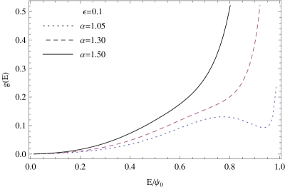
Figure 3: The energy part of the distribution function (left panel) and the differential energy distribution (right panel) of the Generalized Moore model with the constant anisotropy parameter of $\beta=1/2$ and $\epsilon=0.1$: dotted lines ($\alpha=1.05$, where the asymptotic behavior of density profile is similar to the NFW profile’s, but DF doesn’t meet the condition $dg(E)/dE>0$.), dashed lines ($\alpha=1.30$), solid lines ($\alpha=1.50$, closes to the Moore model).

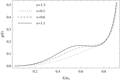
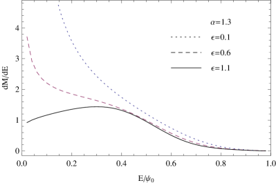
Figure 4: The energy part of the distribution function (left panel) and the differential energy distribution (right panel) of the Generalized Moore model with the constant anisotropy parameter of $\beta=1/2$ and $\alpha=1.3$: dotted lines ($\epsilon=0.1$), dashed lines ($\epsilon=0.6$), solid lines ($\epsilon=1.1$, where DF doesn’t meet the condition $dg(E)/dE>0$).

In this kind of profile, we also calculate $r_{E}$ by numerical way. The $F(E,L)$ and $dM/dE$ are expressed as:

$$\begin{split}&F(E,L)=\ \left.-\frac{B_{4}(r)}{8\pi^{3}L\ B_{5}(r)\Gamma_{1}}\ \frac{B_{6}(r)}{(-3+\alpha)\ A_{7}(r)+\Gamma_{2}\ A_{6}(r)}\right|_{r=r_{E}}\\ &\frac{dM}{dE}=\ \left.-\frac{r^{2}\ B_{4}(r)}{2B_{5}(r)\Gamma_{1}}\ \frac{B_{6}(r)}{(-3+\alpha)\ A_{7}(r)+\Gamma_{2}\ A_{6}(r)}\right|_{r=r_{E}}\ .\end{split}$$ (23)

Fig. 3 and Fig. 4 show $g(E)-E/\psi_{0}$ and $dM/dE-E/\psi_{0}$ for different values of parameters $\alpha$ and $\epsilon$.

Parameters $\epsilon$ and $\alpha_{c}$ $\epsilon=$      $0.01$      $0.1$      $0.2$      $0.3$      $0.4$      $0.5$ $\alpha_{c}\simeq$      $1.110$      $1.127$      $1.146$      $1.166$      $1.186$      $1.209$ $\epsilon=$      $0.6$      $0.7$      $0.8$      $0.9$      $1.0$ $\alpha_{c}\simeq$      $1.230$      $1.253$      $1.276$      $1.299$      $1.323$

In this model, a basic stability condition[35, 36, 37] for the spherical stellar system $dF/dE>0$ is equivalent to the condition $dg(E)/dE>0$ (note: the ”$E$” here is not the energy of a particle but the binding energy). We note that spherical systems with certain $\alpha$ and $\epsilon$ may not meet this condition. This condition requires that the parameter $\alpha_{i}$ should be larger than a critical value $\alpha_{c}$ for the given parameter $\epsilon_{i}$. We calculate $\alpha_{c}$ numerically and show them in Table 3.2. The difference of the two generalized profiles is shown in Fig. 5. One can see that the parameter $\alpha$ controls the asymptotic density profile in the inner parts, while $\epsilon$ is responsible for the asymptotic behavior of the outer profile.

file=Fig5.eps,width=8.5cm

Figure 5: We set $G=1,M_{tot}=1$ and $\beta=1/2$. Two solid lines: New Generalized NFW profiles with different parameters. Two dashed lines: Generalized Moore profiles with different parameters.

4 Discussion and Conclusions

N-body simulations show that the anisotropy parameter $\beta\approx 0.5$ in the outer part of dark matter halos. The distribution functions with constant anisotropy parameter $\beta=1/2$ and the corresponding differential energy distributions can be calculated from the formulae (12). N-body simulations also show that the logarithmic slope of density profile $\gamma=1\sim 1.5$ in the inner part of the dark matter halo ($\rho\sim r^{-\gamma}$).

Many authors work at construction of the dark matter halo models which are better to be analytical, simple, realistic and having flexible anisotropy profile. Unfortunately, it is difficult to meet these requirements at the same time.

In this paper, we only consider the models with constant anisotropy parameter $\beta=1/2$ and then calculate the DFs and DEDs of the two models, the new generalized NFW model and the generalized Moore model. Both have two parameters $\epsilon$ and $\alpha$ for determination of the asymptotic behavior of density profile in the inner and outer parts of the halo. With these two parameters, our models can cover many relatively realistic density profiles which come from N-body simulations. A physical postulate requires that DFs should be positive in the phase space, and our DFs satisfy this basic condition. A basic stability condition for a spherical stellar system $dF/dE>0$ is the sufficient condition for the isotropic case, but is no more a sufficient condition for the anisotropic one.[35, 36, 37] However, we still can use this condition to do some rough discussion. In the new generalized NFW model, all DFs with $\epsilon>0$ and $\alpha=1\sim 1.5$ meet the condition $dF/dE>0$. In the generalized Moore model, we find that not all DFs with $\epsilon>0$ and $\alpha=1\sim 1.5$ satisfy this condition. In order to satisfy the condition $dF/dE>0$, $\alpha_{i}$ should be larger than a critical value $\alpha_{c}$ for a given parameter $\epsilon_{i}$.

We have not dealt with the stability of our models in details in our paper. Although it is difficult to determine the stability domain in the parameter space of the halo model, the study of stability of the stellar system and dark matter halo is very important and some works have already been done [38, 39, 40, 41]. To be more realistic, a more complicated case, the axisymmetric model should be considered[42, 43, 44, 45]. Construction of the polycomponent models is also necessary as the stellar component or the central black hole[46, 47, 28] usually combines with the dark matter component and the two-component models with the stellar and dark matter components were constructed by Ciotti[48].

Although the density profiles of our models are realistic enough and we assume that the anisotropy parameter $\beta=1/2$ from the viewpoint of the simulation, it is still not realistic enough for the anisotropy profile. An $\&$ Evans[33] explored the model whose DF has the form as below,

$$F(E,L)=\sum_{i}L^{-2\beta_{i}}f_{i}(E).$$ (24)

DF is superposition of two or more terms here and this case is more complicated, nevertheless, this kind of DF has more flexible anisotropy profile and it is revealing for our further work to pursue a greater variety of anisotropic behavior of the dark matter halo models.

Appendix A Hypergeometric Function

${}_{p}\tilde{F}_{q}$ is the regularized hypergeometric function which is defined as

$$\ {}_{p}\tilde{F}_{q}(a_{1},...,a_{p};b_{1},...,b_{q};z)\equiv\frac{\ {}_{p}F_{q}(a_{1},...,a_{p};b_{1},...,b_{q};z)}{\Gamma(b_{1})...\Gamma(b_{q})}\ ,$$ (25)

where $\Gamma(z)$ is a gamma function. And ${}_{p}F_{q}(a_{1},...,a_{p};b_{1},...,b_{q};z)$ is the generalized hypergeometric function:

$$\ {}_{p}F_{q}(a_{1},...,a_{p};b_{1},...,b_{q};z)=\sum^{\infty}_{k=0}\frac{(a_{1})_{k}\ (a_{2})_{k}\ ...\ (a_{p})_{k}}{(b_{1})_{k}\ (b_{2})_{k}\ ...\ (b_{q})_{k}}\ \frac{z^{k}}{k!}\ ,$$ (26)

where $(a)_{k}$ is the Pochhammer symbol,

$$(a)_{k}\equiv\frac{\Gamma(a+k)}{\Gamma(a)}=a(a+1)...(a+k-1)\ .$$ (27)

The specific hypergeometric functions can be calculated by mathematical software packages such as Mathematica.

References

- [1] J. F. Navarro, C. S. Frenk and S. D. M. White, Mon. Not. R. Astron. Soc. 275 (1995) 720.
- [2] J. F. Navarro, C. S. Frenk and S. D. M. White, Astrophys. J. 462 (1996) 563.
- [3] B. Moore, T. Quinn, F. Governato, J. Stadel and G. Lake Mon. Not. R. Astron. Soc. 310 (1999) 1147.
- [4] Y. P. Jing and Y. Suto, Astrophys. J. 529 (2000) L69.
- [5] V. Avila-Reese, C. Firmani, A. Klypin and A. V. Kravtsov Mon. Not. R. Astron. Soc. 310 (1999) 527.
- [6] S. H. Hansen and B. Moore, New Astron. 11 (2006) 333.
- [7] S. H. Hansen and J. Stadel, J. Cosmol. Astropart. P. 05 (2006) 014.
- [8] J. J. Binney, Mon. Not. R. Astron. Soc. 190 (1980) 873.
- [9] A. S. Eddington, Mon. Not. R. Astron. Soc. 76 (1916) 572.
- [10] R. W. Michie, Mon. Not. R. Astron. Soc. 125 (1963) 127.
- [11] I. R. King, Astron. J. 71 (1966) 64.
- [12] H. Dejonghe, Phys. Rep. 133 (1986) Nos 3 - 4.
- [13] H. Dejonghe, Mon. Not. R. Astron. Soc. 224 (1987) 13.
- [14] N. W. Evans and J. H. An, Phys. Rev. D 73 (2006) 023524.
- [15] L. P. Osipkov, Pis’ma Astron. Zh. 5 (1979) 77.
- [16] L. P. Osipkov, Soviet Astron. Lett. 5 (1979) 42.
- [17] D. Merritt, Astron. J. 90 (1985) 1027.
- [18] P. Cuddeford, Mon. Not. R. Astron. Soc. 253 (1991) 414.
- [19] L. Ciotti and S. Pellegrini, Mon. Not. R. Astron. Soc. 255 (1992) 561.
- [20] M. Baes and E. van Hese, Astron. Astrophys. 471 (2007) 419.
- [21] C. Tonini, A. Lapi, and P. Salucci, Astrophys. J. 649 (2006) 591.
- [22] H. C. Plummer, Mon. Not. R. Astron. Soc. 71 (1911) 460.
- [23] U. I. K. Veltmann, Astron. Zh. 56 (1979) 976.
- [24] L. Hernquist, Astrophys. J. 356 (1990) 359.
- [25] M. Baes and H. Dejonghe, Astron. Astrophys. 393 (2002) 485.
- [26] W. Dehnen, Mon. Not. R. Astron. Soc. 265 (1993) 250.
- [27] S. Tremaine, D. O. Richstone, Y. Byun, A. Dressler, S. M. Faber, C. Grillmair, J. Kormendy and T. R. Lauer, Astron. J. 107 (1994) 634.
- [28] M. Baes, H. Dejonghe and P. Buyle, Astron. Astrophys. 432 (2005) 411.
- [29] P. Buyle, C. Hunter and H. Dejonghe, Mon. Not. R. Astron. Soc. 375 (2007) 773.
- [30] A. Toomre, Astrophys. J. 259 (1982) 535.
- [31] J. H. An and N. W. Evans, Astron. Astrophys. 444 (2005) 45.
- [32] L. M. Widrow, Astrophys. J. Suppl. Ser. 131 (2000) 39.
- [33] J. H. An and N. W. Evans, Astron. J. 131 (2006) 782.
- [34] M. I. Wilkinson and N. W. Evans, Mon. Not. R. Astron. Soc. 310 (1999) 645.
- [35] V. A. Antonov, Vestn. Leningr. Univ. 7 (1962) 135.
- [36] J. P. Doremus, M. R. Feix and G. Baumann, Phys. Rev.Lett. 26 (1971) 725.
- [37] J. Binney and S. Tremaine, Galactic Dynamics, (Princeton University Press, Princeton, 1987).
- [38] H. Dejonghe and D. Merritt, Astrophys. J. 328 (1988) 93.
- [39] A. Meza and N. Zamorano, Astrophys. J. 490 (1997) 136.
- [40] A. Meza, Astron. Astrophys. 395 (2002) 25.
- [41] P. Buyle, E. Van Hese, S. De Rijcke and H. Dejonghe, Mon. Not. R. Astron. Soc. 375 (2007) 1157.
- [42] C. Hunter and E. Qian, Mon. Not. R. Astron. Soc. 262 (1993) 401.
- [43] K. Holley-Bockelmann, J. C. Mihos, S. Sigurdsson and L. Hernquist, Astrophys. J. 549 (2001) 862.
- [44] B. Famaey, K. Van Caelenberg and H. Dejonghe, Mon. Not. R. Astron. Soc. 335 (2002) 201.
- [45] Z. L. Jiang and L. Ossipkov, Mon. Not. R. Astron. Soc. 379 (2007) 1133.
- [46] D. Merritt and L. Ferrarese, Mon. Not. R. Astron. Soc. 320 (2001) 30.
- [47] M. Baes and H. Dejonghe, Mon. Not. R. Astron. Soc. 351 (2004) 18.
- [48] L. Ciotti, Astrophys. J. 471 (1996) 68.