Four point function of $R$-currents in ${\cal N}=4$ SYM
in the Regge limit at weak coupling

Abstract

We compute, in ${\cal N}=4$ super Yang-Mills theory, the four point correlation function of $R$-currents in the Regge limit in the leading logarithmic approximation at weak coupling. Such a correlator is the closest analog to photon-photon scattering within QCD, and there is a well-defined procedure to perform the analogous computation at strong coupling via the AdS/CFT correspondence. The main result of this paper is, on the gauge theory side, the proof of Regge factorization and the explicit computation of the $R$-current impact factors.

I Introduction

There are many aspects of QCD that are still lacking a satisfying understanding from first principles. One is the behavior in the Regge limit, where the theory is expected to be better formulated in terms of new effective fields, the Reggeized particles Gribov:1968fc ; Lipatov:1996ts . One of the central building blocks of this Reggeon field theory is the Balitsky-Fadin-Kuraev-Lipatov (BFKL) Pomeron which comes as a bound state of two Reggeized gluons with vacuum quantum numbers Kuraev:1976ge-Kuraev:1977fs-Balitsky:1978ic . While the original calculations were done in the leading logarithmic approximation (LLA), the requirement of high precision has led to the computation of subleading corrections (NLO corrections) to the BFKL equation Fadin:1998py ; Camici:1997ij-Ciafaloni:1998gs , and they have been found to be large. While, for finite values of $N_{c}$ further steps beyond NLO will extend beyond the ladder structure and hence open the full complexity of Reggeon field theory, there is evidence that the large-$N_{c}$ limit suppresses the transition from two to four Reggeized gluons and thus allows, also beyond the NLO corrections, to stay within the ladder approximation.

Beside its phenomenological relevance, high energy physics has been a prolific source of theoretical cues. In the early days, the proposal by Veneziano Veneziano:1968yb of crossing-symmetric, Regge behaved amplitude turned out to be a key point for the beginning of the string theory era. Later on, in the early nineties, when studying unitarity corrections to the BFKL Pomeron, Lipatov Lipatov:1993yb ; LiFK found the first occurrence of integrable structures in four dimensional quantum field theories: In the large-$N_{c}$ limit, the generalization of the BFKL evolution equation, the Bartels-Kwiecinski-Praszalowicz (BKP) evolution equations BKP for the $n$ gluon state, were found to be integrable.

Recently, the connection between quantum field theory and string theory was revived by the advent of the AdS/CFT correspondence Maldacena:1997re-Witten:1998qj-Gubser:1998bc . This conjectured connection between Yang-Mills theories (the maximally supersymmetric version of QCD, ${\cal N}=4$ super Yang-Mills theory (SYM), at large $N_{c}$, being the most attractive example) and some string theory (type IIB on $AdS_{5}\times S^{5}$ for the case just mentioned) has motivated, among other directions of interest, also the analysis of the high energy limit in supersymmetric theories, in particular the BFKL Pomeron Kotikov:2000pm-Kotikov:2002ab-Kotikov:2003fb-Kotikov:2004er and the vacuum singularity fromJaniktoHatta .

On the gauge theory side, the most reliable environment of investigating the Pomeron is provided by the scattering of electromagnetic currents, e.g., the total cross section of the scattering of two virtual photons Bartels:1996ke ; Brodsky:1997sd . In order to be able to define correlation functions that are defined on both the gauge theory and the string theory side, it has been suggested CaronHuot:2006te to use, as a substitute of the electromagnetic current, the $R$-currents belonging to the global $SU_{R}(4)$ of the ${\cal N}=4$ SYM theory. To be more precise, one picks a $U(1)$ subgroup of the $SU_{R}(4)$ group. It therefore seems natural to investigate four point correlators (and even $n$ point correlators with $n>4$) of these $R$-current operators, representing correlation functions which are well-defined both on the gauge theory and the string theory side. Whereas two point and three point correlators of the $R$-current operators have been studied before Chalmers:1998xr , an analysis of four point correlation functions has not yet been performed.

In this paper we address, within ${\cal N}=4$ SYM, the Regge limit of $R$-current operators, beginning with the gauge theory side. In QCD it is well known that, in the high energy Regge limit, the four point amplitude of the electromagnetic current factorizes into impact factors of the (virtual) photon and the BFKL Green’s function that describes the energy dependence. In this paper, as a start, we will verify that this expectation remains valid also for the supersymmetric extension, where scalar fields have to be included, and the fermions belong to the adjoint representation of the gauge group. Since the $R$-currents are non-Abelian, their associated Ward identities are more complicated then in QED, and this causes some subtleties in the treatment of UV divergencies. We investigate the one-loop box diagrams and compute, in the leading logarithmic representation, the impact factors of the $R$-current. Since, in the leading logarithmic approximation, the BFKL Green’s function remains the same as in the nonsupersymmetric case, we thus find the supersymmetric analog of the $\gamma^{*}\gamma^{*}$ total cross section discussed in QCD. In a forthcoming paper we will turn to the dual analog on the string theory side where the graviton is expected to play the dominant role.

II Review of photon-photon scattering in QCD

The most convenient way of addressing Regge dynamics in QCD is the study of the elastic scattering of two highly virtual photons. The large virtuality of the external photons provides hard scales that allow us to use perturbation theory. One focuses on the computation of the leading order in the electric charge $\alpha$, at which each photon splits into a quark-antiquark pair, but the order in the strong coupling constant $\alpha_{s}$ can be arbitrary high. The decay of the photon is mediated by the electromagnetic current $j_{\mu}$ associated with the $U(1)$ gauge symmetry of QED. Therefore the computation reduces to evaluating the four point correlation function of this current. In momentum space it reads

$$i(2\pi)^{4}\delta^{(4)}(p_{A}+p_{B}-p_{A^{\prime}}-p_{B^{\prime}})A(s,t)^{\mu_{A}\mu_{B}\mu_{A^{\prime}}\mu_{B^{\prime}}}=$$

$$\qquad\int\prod_{i}d^{4}x_{i}~{}e^{-ip_{A}\cdot x_{A}-ip_{B}\cdot x_{B}+ip_{A^{\prime}}\cdot x_{A^{\prime}}+ip_{B^{\prime}}\cdot x_{B^{\prime}}}$$

$$\qquad\times\langle j^{\mu_{A}}(x_{A})j^{\mu_{B}}(x_{B})j^{\mu_{A^{\prime}}}(x_{A}^{\prime})j^{\mu_{B^{\prime}}}(x_{B}^{\prime})\rangle\,,$$ (1)

where $A$ depends upon the external momenta only through the usual Mandelstam variables $s=(p_{A}+p_{B})^{2}>0$, $t=q^{2}=(p_{A}-p_{A}^{\prime})^{2}\simeq-\mbox{\boldmath$q$}^{2}<0$, and the virtualities of the current momenta $Q_{i}^{2}=-p_{i}^{2}>0$. The Regge limit is defined as

$$s>>|t|,Q_{i}^{2}\,.$$ (2)

We will perform the computation using the Sudakov decomposition of momenta discussed in the appendix. It is convenient to compute the amplitude (II) in terms of its projections onto the polarization vectors of the external photons. The reader is referred to the appendix A.1 for the explicit definition of the polarization vectors in the Regge limit. Once they are defined, we can use their completeness (59) in order to decompose the correlation function (II) as

$$A(s,t)_{\mu_{A}\mu_{B}\mu_{A^{\prime}}\mu_{B^{\prime}}}=$$

$$\qquad\sum_{\lambda_{i}}\epsilon^{\lambda_{A}}_{\mu_{A}}(p_{A})^{*}\epsilon^{\lambda_{B}}_{\mu_{B}}(p_{B})^{*}\epsilon^{\lambda_{A^{\prime}}}_{\mu_{A^{\prime}}}(p_{A^{\prime}})\epsilon^{\lambda_{B^{\prime}}}_{\mu_{B^{\prime}}}(p_{B^{\prime}})$$

$$\qquad\times\langle\lambda_{A}\lambda_{B}|A|\lambda_{A^{\prime}}\lambda_{B^{\prime}}\rangle\,,\quad\lambda_{i}=L,\pm\,,$$ (3)

where $\langle\lambda_{A}\lambda_{B}|A|\lambda_{A^{\prime}}\lambda_{B^{\prime}}\rangle$ are the projections of $A$ onto the appropriate polarization vectors. In the following we will often suppress, for the scattering amplitude $A$ on the LHS, the tensor indices.

II.1 Ward identities

Let us briefly recapitulate the derivation of the Ward identities for the time-ordered product of a conserved current, $j^{\mu}$ (satisfying $\partial_{\mu}j^{\mu}(x)=0$), with some other operators ${\cal O}_{i}$. Because of the theta-functions inserted by the time-ordering operator $T$, there are terms proportional to delta-functions of time differences,

$$\partial_{\mu}Tj^{\mu}(x){\cal O}_{1}(x_{1})...{\cal O}_{n}(x_{n})=$$

$$\sum_{i=1}^{n}\delta(x^{0}-x_{i}^{0})T{\cal O}_{1}(x_{1})...[j^{0}(x),{\cal O}_{i}(x_{i})]...{\cal O}_{n}(x_{n})\,.$$ (4)

From the standard commutation relation one sees that the equal-time commutator of the zero-component of the current with an operator is proportional to the charge of the operator itself under the symmetry group,

$$[j^{0}(\vec{x},t),{\cal O}(\vec{y},t)]=\delta^{(3)}(\vec{x}-\vec{y})q_{{\cal O}}{\cal O}(\vec{x},t)\,.$$ (5)

Here $q_{{\cal O}}$ is the charge of the operator ${\cal O}$ in units of electric charge $e$. Using (5) in (II.1) one obtains the explicit expression of the contact terms:

$$\partial_{\mu}Tj^{\mu}(x){\cal O}_{1}(x_{1})...{\cal O}_{n}(x_{n})=$$

$$\qquad\sum_{i=1}^{n}\delta^{(4)}(x-x_{i})q_{{\cal O}_{i}}T{\cal O}_{1}(x_{1})...{\cal O}_{n}(x_{n})\,.$$ (6)

One sees then that there are no contact terms with neutral operators. In particular, since in an Abelian theory the current is neutral, there are no contact terms in the $T$-products of currents,

$$\partial_{\mu}Tj^{\mu}(x)j^{\mu_{1}}(x_{1})...j^{\mu_{n}}(x_{n})=0\,.$$ (7)

Going to momentum space and taking the vacuum expectation value one gets the well-known equation

$$p_{\mu}\langle j^{\mu}(p)j^{\mu_{1}}(p_{1})...j^{\mu_{n}}(p_{n})\rangle=0\,.$$ (8)

Going from (7) to (8) involves a subtlety. The integrations in the coordinates implied by Fourier transformation pick up contributions from the regions where two or more currents are at the same point. In some cases the product of currents at the same point requires some care, scalar QED is a simple example (Sec.III.3).

II.2 Box diagrams

The lowest order diagrams in Fig. 1 contributing to the correlation function $A$ are fermionic boxes (one-loop).

$$A^{(0)}_{B}=$$

$$\begin{minipage}{62.59596pt} \includegraphics[width=62.59596pt]{pics/sBoxQED.eps} \end{minipage}+\begin{minipage}{62.59596pt} \includegraphics[width=62.59596pt]{pics/tBoxQED.eps} \end{minipage}+\begin{minipage}{62.59596pt} \includegraphics[width=62.59596pt]{pics/uBoxQED.eps} \end{minipage}\,.$$

Figure 1: Lowest order diagrams

At high energies, they behave as $\log^{2}s$ Bartels:2003dj , and therefore give a contribution to the total cross section which decreases as $1/s$. Radiative gluonic corrections to these fermion loop graphs will not modify the power of the energy dependence but provide double logarithmic corrections.

II.3 Two gluon exchange

At the three-loop level a new class of diagrams becomes available, in which purely gluonic $t$-channel states appear. As an example, two lowest order diagrams are shown in Fig. 2.

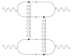
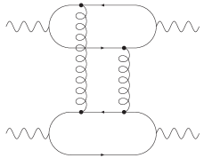
Figure 2: An example of three-loop diagrams corresponding to two gluon exchange.

At high energies the sum of all lowest order diagrams, $A$, behaves as $\alpha_{s}^{2}s$, and therefore provides a contribution to the total cross section which (up to powers of $\ln s$) is constant in $s$. It is clear that at high energy, independently of how small $\alpha_{s}$ is, these diagrams dominate with respect to the boxes and their radiative corrections. In the Regge limit the lowest order diagram, $A^{(0)}$, is purely imaginary and takes the form

$$A^{(0)}(s,t)=$$ (9)

$$is\int\frac{d^{2}\mbox{\boldmath$k$}}{(2\pi)^{2}\mbox{\boldmath$k$}^{2}(\mbox{\boldmath$q$}-\mbox{\boldmath$k$})^{2}}\Phi^{a_{1}a_{2}}_{A}(\mbox{\boldmath$k$},\mbox{\boldmath$q$}-\mbox{\boldmath$k$})\Phi^{a_{1}a_{2}}_{B}(\mbox{\boldmath$k$},\mbox{\boldmath$q$}-\mbox{\boldmath$k$})\,.$$

Here the so called impact factors $\Phi$ (Fig. 3) represent the coupling of the virtual photons to the two $t$-channel gluons. Their precise definition is

$$\Phi^{\lambda_{A}\lambda_{A^{\prime}}aa^{\prime}}_{A}(\mbox{\boldmath$k$},\mbox{\boldmath$k$}^{\prime})=\frac{1}{s^{2}}\epsilon^{\lambda_{A}}_{\mu_{A}}(p_{A})^{*}\epsilon^{\lambda_{A^{\prime}}}_{\mu_{A^{\prime}}}(p_{A^{\prime}})~{}p_{2\rho}p_{2\rho^{\prime}}$$

$$\qquad\times\int\frac{ds_{1}}{2\pi}\operatorname{Im}A^{\mu_{A}\mu_{A^{\prime}}\rho\rho^{\prime}}_{\gamma q\to\gamma q}(s_{1},t)$$ (10)

with a similar definition for $\Phi_{B}$. Here $\operatorname{Im}A^{\mu_{A}\mu_{A^{\prime}}\rho\rho^{\prime}}_{\gamma q\to\gamma q}(s_{1},t)$ is the imaginary part of the amplitude for the scattering of the virtual photon $A$ with polarization $\lambda_{A}$ and a gluon with momentum $-k$, Lorenz index $\rho$, and color label $a$ into the photon $A^{\prime}$ with polarization $\lambda_{A^{\prime}}$ and a gluon with momentum $k$, Lorenz index $\rho^{\prime}$, and color label $a^{\prime}$. $s_{1}$ is the total energy squared of the photon-gluon system, and it is related to the Sudakov component $\beta$ of $k$ (which in this regime is the same as the one of $k^{\prime}$) along the Sudakov vector $p_{2}$ by $s_{1}=(p_{A}-k)^{2}\simeq-Q_{A}^{2}-\mbox{\boldmath$k$}^{2}-s\beta\approx-s\beta$. For each $t$-channel gluon, we have a factor $2p_{2\rho}p_{1\sigma}/s$, since, in the Regge limit, only a specific component of the gluon polarization tensor contributes to the leading power in $s$, namely,

$$g_{\rho\sigma}=\frac{2}{s}\big{(}p_{2\rho}p_{1\sigma}+p_{1\rho}p_{2\sigma}\big{)}+g_{\perp\rho\sigma}\to\frac{2}{s}p_{2\rho}p_{1\sigma}\,.$$ (11)

With these definitions the impact factors $\Phi_{A,B}$ are independent of $s$. They depend, in the leading approximation we are interested in, only upon the virtuality and the polarizations of the photons, the gluon colors, and the transverse momenta.

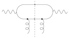
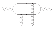
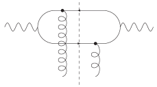
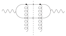
Figure 3: The one-loop diagrams contributing to the impact factor $\Phi$.

II.4 All-order summation in the leading logarithmic approximation

Generalizing, in the leading logarithmic approximation, the lowest order diagrams to higher orders in $\alpha_{s}$, the two gluon exchange is replaced by the BFKL Kuraev:1976ge-Kuraev:1977fs-Balitsky:1978ic Green’s function:

$$A(s,t)=is~{}\Phi_{A}\otimes G(s)\otimes\Phi_{B}\,,$$ (12)

where we have introduced the symbol $\otimes$ to denote the transverse momentum convolution of (9), including the transverse gluon propagators and the contraction of the color indices. $G(s)$ is the Green’s function of the BFKL equation, accounting for the resummed LL corrections. The LLA sums the radiative corrections to $A^{(0)}$ in (9), and it is valid in the region where $\alpha_{s}\ll 1$ and $\alpha_{s}\log s\sim 1$. The BFKL Pomeron denotes the bound state formed by two interacting Reggeized gluons with the quantum numbers of the vacuum (for more details see, for example, Lipatov:1989bs ; Lipatov:1996ts ; Forshaw:1997dc and references therein). In LLA, the BFKL Green’s function contains only gluonic contributions; fermionic corrections appear only in the next-to-leading correction. As a consequence of this, when turning to the supersymmetric extension of QCD, the LLA of the BFKL Pomeron remains the same as in QCD. What needs to be studied is the role of the scalar degrees of freedom in the box diagrams and in the impact factors. This will be done in the following section.

III ${\cal N}=4$ SYM and $R$-currents

The maximally supersymmetric non-Abelian gauge theory in four dimensions admits ${\cal N}=4$ supersymmetries. It contains a vector multiplet in the adjoint representation of the gauge group $SU(N_{c})$. The theory enjoys a $SU_{R}(4)$  global symmetry, called $R$-symmetry, which transforms the different supercharges. In terms of component fields the theory has

• 1 vector field $A_{\mu}$, scalar of $SU_{R}(4)$;

• 4 chiral spinors $\lambda_{I}$ in the fundamental representation of $SU_{R}(4)$;

• 6 real scalars $X_{M}$ in the vector representation of $SU_{R}(4)$.

Capital indices transform under the $R$-symmetry group. In particular, $A,B,C,...=1,...,15$ are indices of the adjoint representation, $I,J,K,...=1,...,4$ transform under the fundamental, and $M,N,...=1,...,6$ under the vector representations of the $R$-symmetry. Small indices $a,b,c,...=1,...,N_{c}^{2}-1$ are adjoint representation indices for the gauge group $SU(N_{c})$. Since all the fields live in the adjoint representation of $SU(N_{c})$, we can write $\Phi=\Phi_{ab}=\Phi^{c}(t^{c})_{ab}$, with $(t^{c})_{ab}=-if^{acb}$ with $f^{abc}$ being the $SU(N_{c})$  structure constants, $[t^{a},t^{b}]=if^{abc}t^{c}$. Our convention for the normalization of the generators $t^{a}$ is such that $\operatorname{tr}(t^{a}t^{b})=\delta^{ab}/2$.

The Lagrangian is Brink:1976bc

$${\cal L} = \operatorname{tr}\Big{(}-\frac{1}{2}F_{\mu\nu}F^{\mu\nu}+D_{\mu}X_{M}D^{\mu}X_{M}+2i\lambda_{I}\sigma^{\mu}D_{\mu}\bar{\lambda}^{I}$$ (13)

$$-2ig\lambda_{I}[\lambda_{J},X^{IJ}]-2ig\bar{\lambda}^{I}[\bar{\lambda}^{J},X_{IJ}]$$

$$+\frac{1}{2}g^{2}[X_{M},X_{N}][X_{M},X_{N}]\Big{)},$$

where $X_{M}$ and $X_{IJ}$ are related by the $SU(4)\cong SO(6)$ sigma symbols:

$$X_{IJ}=-\frac{1}{2}(\Sigma_{M})_{IJ}X_{M}\,,\qquad X^{IJ}=\frac{1}{2}(\Sigma^{-1}_{M})^{IJ}X_{M}\,,$$ (14)

with $\operatorname{Tr}(\Sigma_{M}\Sigma_{N}^{-1})=4\delta_{MN}$, which implies that  $X_{M}X_{M}=X_{IJ}X^{IJ}$. The covariant derivative $D_{\mu}$ and the gauge field strength tensor $F_{\mu\nu}$ are defined as usual by

$$D_{\mu}\Phi = \partial_{\mu}\Phi-ig[A_{\mu},\Phi]\,,$$ (15)

$$F_{\mu\nu} = \partial_{\mu}A_{\nu}-\partial_{\nu}A_{\mu}-ig[A_{\mu},A_{\nu}]\,.$$ (16)

III.1 $R$-symmetry currents and the four point function

The Lagrangian (13) is invariant under the global transformation ($R$-symmetry)

$$\Bigg{\{}\begin{array}[]{lcl}\delta\lambda^{a\alpha I}&=&i\epsilon_{A}\lambda^{a\alpha J}(T^{A})_{JI}\,,\\ \delta\bar{\lambda}^{a\dot{\alpha}I}&=&-i\epsilon_{A}(T^{A})_{IJ}\bar{\lambda}^{a\dot{\alpha}J}\,,\\ \delta X^{a}_{M}&=&i\epsilon_{A}(T^{A})_{MN}X^{a}_{N}\,,\end{array}$$ (17)

where $\epsilon_{A}$ are small parameters, and $T^{A}$ are the $SU_{R}(4)$  generators in the appropriate representation.

The Noether current of the symmetry is

$$J_{R}^{\mu A}=i\frac{\partial{\cal L}}{\partial(\partial_{\mu}\Phi)}\Delta^{A}\Phi=\operatorname{tr}\Big{(}-\lambda\sigma^{\mu}T^{A}\bar{\lambda}-iXT^{A}D^{\mu}X\Big{)}\,,$$ (18)

where $\Delta^{A}\Phi$ is obtained from (17) with the definition $\delta\Phi=i\epsilon_{A}\Delta^{A}\Phi$ for an infinitesimal $R$-transformation.

We are interested in evaluating the momentum space four point function defined in analogy to (II),

$$i(2\pi)^{4}\delta(p_{A}+p_{B}-p_{A^{\prime}}-p_{B^{\prime}})A_{R}(s,t)^{\mu_{A}\mu_{B}\mu_{A^{\prime}}\mu_{B^{\prime}}}=$$

$$\int\prod_{i}d^{4}x_{i}~{}e^{-ip_{A}\cdot x_{A}-ip_{B}\cdot x_{B}+ip_{A^{\prime}}\cdot x_{A^{\prime}}+ip_{B^{\prime}}\cdot x_{B^{\prime}}}$$

$$\times\langle J_{R}^{A\mu_{A}}(x_{A})J_{R}^{B\mu_{B}}(x_{B})J_{R}^{A^{\prime}\mu_{A^{\prime}}}(x_{A}^{\prime})J_{R}^{B^{\prime}\mu_{B^{\prime}}}(x_{B}^{\prime})\rangle$$ (19)

at weak coupling in the Regge limit (2).

III.2 Ward identities

From (II.1) and (5) we can compute explicitly the Ward identities satisfied by (III.1). We only need to specialize (5) to the case of interest:

$$[J_{R}^{A0}(\vec{x},t),J_{R}^{B\mu}(\vec{y},t)]=\delta^{(3)}(\vec{x}-\vec{y})(T^{A})^{B}_{C}J_{R}^{C\mu}(\vec{x},t)\,.$$ (20)

The nonvanishing of the commutators (20), which is due to the fact that conserved currents of a non-Abelian symmetry are charged, implies immediately that also the contact terms in the Ward identities do not vanish,

$$\partial_{\mu}\langle J_{R}^{A\mu}(x)J_{R}^{A_{1}\mu_{1}}(x_{1})...J_{R}^{A_{n}\mu_{n}}(x_{n})\rangle=\sum_{i=1}^{n}\delta^{(4)}(x-x_{i})$$

$$\times\langle J_{R}^{A_{1}\mu_{1}}(x_{1})...(T^{A})^{A_{i}}_{C}J_{R}^{C\mu_{i}}(x)...J_{R}^{A_{n}\mu_{n}}(x_{n})\rangle\,.$$ (21)

Compared to the QCD case, this introduces some additional complications. In particular, the standard computation according to which the four point function is finite, despite näive power counting which suggests a logarithmic divergence, does not apply anymore. Explicit computation shows that the UV poles still cancel, but now as a result of the interplay between the scalar and fermionic sectors (Sec. III.4). It is therefore a consequence of supersymmetry.

The change of the Ward identities, at first sight, also affects our use of the polarization vectors. The simplifications which lead from (63-68) to (69-73) were only possible because of the simple Ward identities (8), and the more complicated identities (III.2) spoil this argument. If, however, instead of the full $SU_{R}(4)$  group we restrict ourselves to a $U(1)$ subgroup of $SU_{R}(4)$, we reach a situation similar to the QCD case. Restriction to the $U(1)$ means that, on the RHS of (III.2), all $(T^{A})^{A_{i}}_{C}=-if^{AA_{i}C}$ vanish, and one recovers the same Ward identities without contact terms as in QCD:

$$\partial_{\mu}\langle J_{R}^{\mu}(x)J_{R}^{\mu_{1}}(x_{1})...J_{R}^{\mu_{n}}(x_{n})\rangle=0\,.$$ (22)

We therefore can proceed as before and, via Eq. (II), conveniently compute projections of $A_{R}$ onto specific polarization vectors.

III.3 An excursion into scalar QED

As we mentioned already at the end of Sec. II.1, working in Fourier space requires some care with renormalization. The problem can be easily illustrated in the simple framework of scalar QED. Let us consider, as an example, the two point function $A_{2}=\langle j_{\mu}(x)j_{\nu}(y)\rangle$ of the electromagnetic current $j_{\mu}=i(\varphi\partial_{\mu}\varphi^{*}-\varphi^{*}\partial_{\mu}\varphi)-2eA_{\mu}\varphi^{*}\varphi$. Again, $U(1)$ gauge symmetry implies the Ward identity $\partial_{\mu}\langle j_{\mu}(x)j_{\nu}(y)\rangle=0$. The computation of the lowest order in perturbation theory performed in the coordinate space with $x\neq y$, would involve just one diagram, Fig. 4.

$$A_{2\mu\nu}^{(0)}(x,y)=\begin{minipage}{142.26378pt} \includegraphics[width=142.26378pt]{pics/2pointSQED.eps} \end{minipage}\,.$$

Figure 4: Lowest order diagram contributing to the two point function of the electromagnetic current.

Going to momentum space, this diagram gives

$$A_{2\mu\nu}^{(0)}(p)=\int\frac{d^{d}k}{(2\pi)^{d}}\frac{(2k-p)_{\mu}(2k-p)_{\nu}}{k^{2}(k-p)^{2}}\,.$$ (23)

One immediately sees that (23) does not satisfy the Ward identity,

$$p^{\mu}A_{2\mu\nu}^{(0)}(p)=2p_{\nu}\int\frac{d^{d}k}{(2\pi)^{d}}\frac{1}{k^{2}}\,.$$ (24)

The problem arises because the product of two currents in $A_{2}$ is not regular when $x\to y$. As it is well known, such a product is defined by an operator product expansion (OPE),

$$j_{\mu}(x)j_{\nu}(y)\mathop{\longrightarrow}\limits_{x\to y}{\textstyle\sum_{i}}C_{i}\frac{{\cal O}_{i}(y)}{(x-y)^{\alpha_{i}}}\,,$$ (25)

where ${\cal O}_{i}$ are operators with the same quantum numbers as $j_{\mu}j_{\nu}$. Equation (25) means that the product of two currents at the same point mixes with the operators ${\cal O}_{i}$. By dimensional analysis it is easy to spot the operator which, in (25), gives the leading singularity:

$$j_{\mu}(x)j_{\nu}(y)=C~{}\frac{(g_{\mu\nu}\varphi^{*}\varphi)(y)}{(x-y)^{d}}+{\cal O}\big{(}(x-y)^{-d+2}\big{)}\,.$$ (26)

Note that such singular behavior is precisely on the boundary of convergence of the Fourier integrals, and all the other terms in the OPE contain integrable singularities. It is therefore enough to regularize the divergence by removing this leading term:

$$j_{\mu}(x)j_{\nu}(y)\to j_{\mu}(x)j_{\nu}(y)-C~{}\frac{(g_{\mu\nu}\varphi^{*}\varphi)(y)}{(x-y)^{d}}\,.$$ (27)

In momentum space the operator $g_{\mu\nu}\varphi^{*}\varphi$ leads, at the one-loop level, to an additional diagram..

$$A_{2\mu\nu}^{(0)}[g_{\mu\nu}\varphi^{*}\varphi](x,y)=\begin{minipage}{71.13188pt} \includegraphics[width=71.13188pt]{pics/2pointSQEDPhiPhi.eps} \end{minipage}$$

$$\qquad=-Cg_{\mu\nu}\int\frac{d^{d}k}{(2\pi)^{d}}\frac{1}{k^{2}}\,.$$ (28)

Comparing (III.3) with (24) we can fix $C=2$. With this we obtain, for $A_{2\mu\nu}^{(0)}$, the same result that one would get from computing the one-loop correction of the photon self energy $\langle A_{\mu}A_{\nu}\rangle$ in scalar QED, which indeed satisfies the Ward identity $p^{\mu}A_{2\mu\nu}^{(0)}(p)=0$.

The same argument applies to the scalar sector of the ${\cal N}=4$ theory. One has to add the appropriate regularizing diagrams, which ensure that the correlation functions are well defined and fulfill the Ward identities in momentum space.

Before returning to the ${\cal N}=4$ theory, we observe that the QED computation we just sketched would simplify considerably if we were interested only in the imaginary part of $A_{2}$. The term in (III.3) is real and does not contribute, while the imaginary part of (23), which is easily computed by means of the cutting rules, now fulfills the Ward identity, thanks to the delta-functions of the two on-shell scalar propagators.

III.4 One-loop diagrams

An important step in checking the Regge factorization of the $R$-current scattering amplitude is to verify that the fermionic and scalar one-loop diagrams are subleading at high energies. This task includes the correct regularization of ultraviolet divergencies. For correlators of $R$-currents which belong to a $U(1)$ subgroup, we will show that this task can be solved by applying the previous arguments. When considering a correlation function with arbitrary $SU_{R}(4)$  labels the situation is not as simple as in QCD or scalar QED. The usual argument for the absence of UV divergencies is based on the Ward identities (8) and does not work in the present case. Nevertheless, by performing the explicit computation, we can prove that the one-loop diagrams are UV finite. It will be shown that, in this situation, it is supersymmetry that constrains the UV divergence to be absent. More precisely, it is the interplay between the fermionic and scalar sectors which leads to cancellations.

UV poles

The one-loop fermionic diagrams are the same boxes as in QCD, depicted in Fig. 5.

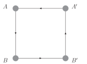
BF1

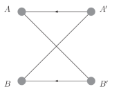
BF2

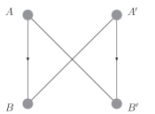
BF3

Figure 5: One-loop diagrams with fermions

In order to discuss their UV behavior, we regularize the IR region by giving the fermions a small mass $m$. The UV singularities of the diagrams $BF1-3$ can be easily computed:

$$BF1_{UV}=\frac{2}{3}\frac{i\pi^{2-\epsilon}m^{-2\epsilon}}{(2\pi)^{4}}\Gamma(\epsilon)\operatorname{Tr}\Big{(}T^{A}T^{A^{\prime}}T^{B^{\prime}}T^{B}\Big{)}$$ (29)

$$\times\Big{(}g_{\mu_{A}\mu_{A^{\prime}}}g_{\mu_{B}\mu_{B^{\prime}}}+g_{\mu_{A}\mu_{B}}g_{\mu_{A^{\prime}}\mu_{B^{\prime}}}-2g_{\mu_{A}\mu_{B^{\prime}}}g_{\mu_{A^{\prime}}\mu_{B}}\Big{)}\,.$$

The contributions $BF2_{UV}$ and $BF3_{UV}$ can be obtained from (29) by permuting indices. It is immediately clear that their sum does not vanish unless we restrict ourselves to the $U(1)$ subgroup, and all the $SU_{R}(4)$ traces are the same. In this case the cancellation works precisely as in QCD.

There are 12 one-loop scalar diagrams (including those which are required for regularization), and they are all depicted in Fig. 6.

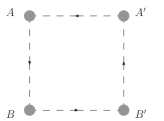
BS1

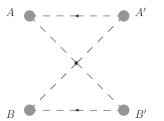
BS2

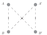
BS3

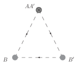
BS4

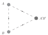
BS5

BS6

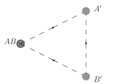
BS7

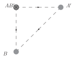
BS8

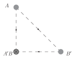
BS9

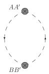
BS10

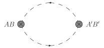
BS11

BS12

Figure 6: One-loop diagrams with scalars

From the UV region of these diagrams one obtains

$$BS1_{UV}=\frac{2}{3}\frac{i\pi^{2-\epsilon}m^{-2\epsilon}}{(2\pi)^{4}}\Gamma(\epsilon)\operatorname{Tr}\Big{(}T^{A}T^{A^{\prime}}T^{B^{\prime}}T^{B}\Big{)}$$ (30)

$$\times\Big{(}g_{\mu_{A}\mu_{A^{\prime}}}g_{\mu_{B}\mu_{B^{\prime}}}+g_{\mu_{A}\mu_{B}}g_{\mu_{A^{\prime}}\mu_{B^{\prime}}}+g_{\mu_{A}\mu_{B^{\prime}}}g_{\mu_{A^{\prime}}\mu_{B}}\Big{)}\,,$$

$$BS4_{UV}=-2\frac{i\pi^{2-\epsilon}m^{-2\epsilon}}{(2\pi)^{4}}\Gamma(\epsilon)$$ (31)

$$\qquad\times\operatorname{Tr}\Big{(}\frac{T^{A}T^{A^{\prime}}+T^{A^{\prime}}T^{A}}{2}T^{B^{\prime}}T^{B}\Big{)}g_{\mu_{A}\mu_{A^{\prime}}}g_{\mu_{B}\mu_{B^{\prime}}}\,,$$

$$BS10_{UV}=2\frac{i\pi^{2-\epsilon}m^{-2\epsilon}}{(2\pi)^{4}}\Gamma(\epsilon)$$ (32)

$$\qquad\times\operatorname{Tr}\Big{(}\frac{T^{A}T^{A^{\prime}}+T^{A^{\prime}}T^{A}}{2}\frac{T^{B}T^{B^{\prime}}+T^{B^{\prime}}T^{B}}{2}\Big{)}$$

$$\qquad\qquad\qquad\qquad\qquad\qquad\qquad\qquad\times g_{\mu_{A}\mu_{A^{\prime}}}g_{\mu_{B}\mu_{B^{\prime}}}\,.$$

All the other diagrams in Fig. 6 can be obtained by permutations of the indices.

When we restrict ourselves to a $U(1)$ subgroup of $SU_{R}(4)$  (which also ensures (22) to hold) all the traces in (29-32) coincide, and the UV poles in the scalar sector cancel among themselves.

In the case of different $SU_{R}(4)$  generators in (29)-(32) the cancellation of the UV poles does not work for the scalar and fermionic sectors separately. But a straightforward computation shows that the sum of the divergent pieces of all scalar diagrams, $BS1-12_{UV}$, is just the opposite of the sum of the fermionic divergencies, $BF1-3_{UV}$, and therefore the full one-loop function is UV finite. This cancellation is a result of the supersymmetry.

High energy behavior

Let us now turn to the calculation of the high energy behavior. From now on, we restrict the $R$-currents to a $U(1)$ subgroup. The computation of the fermion boxes at high energy then is just the same as in QCD. We briefly recall the argument of Gorshkov:1966ht (see also Bartels:2003dj ), which shows how a double log emerges. This will also help to prepare the subsequent computation of the scalar diagrams.

The double log arises because, in the high energy limit, the fermion numerator produces a term proportional to $sk^{2}$. More precisely, the region of integration where the double log arises is $Q_{i}^{2},\mbox{\boldmath$q$}^{2}\ll\mbox{\boldmath$k$}^{2}\ll\alpha s,\beta s$ and $x_{i}\ll\alpha,\beta\ll 1$, with $x_{i}=Q_{i}^{2}/s$. In this region the integral is

$$BF1_{L}=-\frac{s}{2(2\pi)^{4}}\int d\alpha\int d\beta\int d^{2}\mbox{\boldmath$k$}$$

$$\times\frac{s}{(s\alpha\beta-(\mbox{\boldmath$k$}-\mbox{\boldmath$q$})^{2}+i\epsilon)(-s\beta+i\epsilon)(s\alpha+i\epsilon)}\,,$$ (33)

where one of the propagators ($k^{2}$) has been canceled by the $k^{2}$ in the numerator. Closing the $\beta-$contour below we pick up the pole in the first propagator, and after a shift in $k$ we obtain

$$BF1_{L}=-\frac{i}{2(2\pi)^{3}}\int_{x}^{1}\frac{d\alpha}{\alpha}\int_{x}^{1}\frac{d\beta}{\beta}\int d^{2}\mbox{\boldmath$k$}~{}\delta(s\alpha\beta-\mbox{\boldmath$k$}^{2})\,,$$ (34)

where $x=Q^{2}/s\simeq x_{i}$. Performing the angular integration and then the $\mbox{\boldmath$k$}^{2}$ integral via the delta-function we arrive at

$$BF1_{L}=-\frac{i}{4(2\pi)^{2}}\int_{x}^{1}\frac{d\alpha}{\alpha}\int_{x/\alpha}^{1}\frac{d\beta}{\beta}=-\frac{i}{8(2\pi)^{2}}\log^{2}\frac{s}{Q^{2}}\,,$$ (35)

which confirms our previous claim about the double log behavior of the fermion box.

Now we focus on the scalar diagram $BS1$,

$$BS1 = \int\frac{d^{4}k}{(2\pi)^{4}}\frac{(2k-p_{A})_{\mu_{A}}(2k+p_{B})_{\mu_{B}}}{k^{2}(k-q)^{2}}$$ (36)

$$\times\frac{(2k-q-p_{A})_{\mu_{A^{\prime}}}(2k-q+p_{B})_{\mu_{B^{\prime}}}}{(k-p_{A})^{2}(k+p_{B})^{2}}\,.$$

Projecting first onto longitudinal polarizations and keeping only the leading contribution, we obtain

$$BS1_{L}^{LLLL} = Q_{A}Q_{A^{\prime}}Q_{B}Q_{B^{\prime}}\int\frac{d^{4}k}{(2\pi)^{4}}$$ (37)

$$\times\frac{1}{k^{2}(k-q)^{2}(k-p_{A})^{2}(k+p_{B})^{2}}\,,$$

which means that the longitudinal projection reduces simply to the standard scalar integral we would encounter in a massless $\phi^{3}$ theory. It behaves again as a double log, but now the additional logarithm arises in the infrared region $\mbox{\boldmath$k$}\simeq 0$ due to the vanishing mass of the fields. Let us consider indeed the region of integration $x_{i}\ll\alpha,\beta\ll 1$ (which we have already used in order to get to (37)) but $\mbox{\boldmath$k$}^{2}\ll Q_{i}^{2},\mbox{\boldmath$q$}^{2}$. There (37) becomes

$$BS1_{L}^{LLLL}=\frac{sQ_{A}Q_{A^{\prime}}Q_{B}Q_{B^{\prime}}}{2(2\pi)^{4}}\int d\alpha\int d\beta\int d^{2}\mbox{\boldmath$k$}$$

$$\quad\quad\times\frac{1}{(s\alpha\beta-\mbox{\boldmath$k$}^{2}+i\epsilon)(-\mbox{\boldmath$q$}^{2})(-s\beta+i\epsilon)(s\alpha)}\,.$$ (38)

Again we close the $\beta-$contour below and pick up the pole from the first propagator, which is now $k^{2}$

$$BS1_{L}^{LLLL} = -\frac{iQ_{A}Q_{A^{\prime}}Q_{B}Q_{B^{\prime}}}{4(2\pi)^{2}s\mbox{\boldmath$q$}^{2}}$$ (39)

$$\times\int_{x}^{1}\frac{d\alpha}{\alpha}\int_{x}^{1}\frac{d\beta}{\beta}\int_{\mbox{\boldmath$k$}^{2}\ll Q^{2}}d\mbox{\boldmath$k$}^{2}\delta(s\alpha\beta-\mbox{\boldmath$k$}^{2})$$

$$= -\frac{iQ_{A}Q_{A^{\prime}}Q_{B}Q_{B^{\prime}}}{4(2\pi)^{2}s\mbox{\boldmath$q$}^{2}}\int_{x}^{1}\frac{d\alpha}{\alpha}\int_{x}^{x/\alpha}\frac{d\beta}{\beta}$$

$$\simeq \frac{i}{8(2\pi)^{2}}\frac{Q^{2}}{s}\log^{2}\frac{s}{Q^{2}}\,.$$

Let us consider now transverse polarization. Projecting (36) onto the transverse polarization (71-73) and keeping only leading terms in the numerator, we obtain

$$BS1_{L}^{TTTT}=16\int d^{4}k\frac{k\cdot\epsilon^{h_{A}}k\cdot\epsilon^{h_{A^{\prime}}}k\cdot\epsilon^{h_{B}}k\cdot\epsilon^{h_{B^{\prime}}}}{k^{2}(k-q)^{2}(k-p_{A})^{2}(k+p_{B})^{2}}$$

$$=\big{(}\delta^{h_{A}h_{A^{\prime}}}\delta^{h_{B}h_{B^{\prime}}}+\delta^{h_{A}h_{B}}\delta^{h_{A^{\prime}}h_{B^{\prime}}}+\delta^{h_{A}h_{B^{\prime}}}\delta^{h_{A^{\prime}}h_{B}}\big{)}$$

$$\qquad\qquad\times\frac{s}{3(2\pi)^{4}}\int d\alpha\int d\beta\int d^{2}\mbox{\boldmath$k$}$$

$$\qquad\qquad\times\frac{s\alpha\beta-\mbox{\boldmath$k$}^{2}}{(s\alpha\beta-(\mbox{\boldmath$k$}-\mbox{\boldmath$q$})^{2}+i\epsilon)(-s\beta+i\epsilon)(s\alpha)}\,.$$ (40)

As we did in (III.4) we close the $\beta-$contour below and get the residue from the pole in the first propagator, which, after a shift in $k$, gives

$$BS1_{L}^{TTTT}=$$

$$\big{(}\delta^{h_{A}h_{A^{\prime}}}\delta^{h_{B}h_{B^{\prime}}}+\delta^{h_{A}h_{B}}\delta^{h_{A^{\prime}}h_{B^{\prime}}}+\delta^{h_{A}h_{B^{\prime}}}\delta^{h_{A^{\prime}}h_{B}}\big{)}$$

$$\qquad\times\frac{i}{3(2\pi)^{3}s}\int\frac{d\alpha}{\alpha}\int\frac{d\beta}{\beta}\int d^{2}\mbox{\boldmath$k$}$$

$$\qquad\times(s\alpha\beta-\mbox{\boldmath$k$}^{2}-\mbox{\boldmath$q$}^{2}-2\mbox{\boldmath$k$}\cdot\mbox{\boldmath$q$})\delta(s\alpha\beta-\mbox{\boldmath$k$}^{2})\,.$$ (41)

The scalar product vanishes after angular integration, the combination $s\alpha\beta-\mbox{\boldmath$k$}^{2}$ is set to $0$ through the delta-function, and the only term left gives

$$BS1_{L}^{TTTT}\simeq$$

$$-\big{(}\delta^{h_{A}h_{A^{\prime}}}\delta^{h_{B}h_{B^{\prime}}}+\delta^{h_{A}h_{B}}\delta^{h_{A^{\prime}}h_{B^{\prime}}}+\delta^{h_{A}h_{B^{\prime}}}\delta^{h_{A^{\prime}}h_{B}}\big{)}$$

$$\qquad\times\frac{i}{6(2\pi)^{2}}\frac{Q^{2}}{s}\log^{2}\frac{s}{Q^{2}}\,.$$ (42)

Similar computations can be performed for all the other diagrams in Fig. 6, and the results are similar to the one just outlined. This completes our derivation of the leading high energy behavior of all the one-loop diagrams of Fig. 5 and 6.

We would like to stress the importance of the region $\mbox{\boldmath$k$}^{2}\sim s$: at first sight, the numerators in (III.4) and (39) seem to lead to an even stronger behavior than the one we have computed. However, in the limit of large $s$, this region coincides with the UV region which has been discussed at the beginning of this section. These leading terms cancel when all the diagrams are summed over, in the same fashion as the cancellation of the UV poles discussed earlier.

As we will see in the next section, the high energy behavior is dominated by gluon exchange, and the fermion and the scalar box diagrams provide subleading corrections. This is to be expected since, once the UV finiteness of the one-loop diagrams has been verified, we can apply the spin argument, according to which the exchange of two field quanta of spin $s$ leads, in the scattering amplitude, to the high energy behavior $\sim s^{2s-1}$. This implies that also higher order diagrams in which the box diagrams in Fig. 5 are “dressed”, for examples, by gluon rungs, will have the same power behavior in $s$, modified by powers of $\ln^{2}s$ (details can be found in  Bartels:2003dj ). A similar consideration applies to diagrams obtained by “dressing” the scalar loops. For the leading high energy behavior we are thus left with gluon exchanges: using the spin argument one expects, for the scattering amplitude, the high energy behavior$\sim s$.

III.5 Two gluon exchange

As it was the case in QCD, gluon exchange starts at three loops. In Fig. 7 we depict one of the lowest order diagrams contributing to the two gluon exchange, in order to set the notation for the momenta.

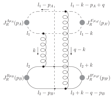
Figure 7: One of the diagrams contributing to the two gluon exchange in ${\cal N}=4$.

Again, we consider the imaginary part (or, equivalently, the discontinuity in $s$). Then we have, in all diagrams, four delta-functions imposing the mass-shell condition for the intermediate particles (either scalars or fermions). Two delta-functions are used to fix the integrations over the longitudinal components of $k$ (the integral in the subenergy $s_{1}$ in (II.3)), and the other two fix one of the two longitudinal integrations inside each of the impact factors. The LL contribution arises from the Regge kinematics, in which $\alpha$ is negligible compared to $\alpha_{1}$, and $\beta$ is negligible compared to $\beta_{2}$. Therefore the subdiagrams belonging to the upper impact factor (scalar loop in Fig. 7) are independent of $\alpha$, and those of the lower impact factor (the fermion loop) are independent of $\beta$. This is the mechanism behind the factorization of (9). In the Regge kinematics also the longitudinal components of the transverse momentum $q$ are small, $\alpha_{q},\beta_{q}\sim 1/s$, and dropping them influences only terms suppressed by powers of $s$.

It is convenient to introduce the notation

$$\Phi^{\lambda\lambda^{\prime}aa^{\prime}}=N_{c}\alpha_{s}\delta^{aa^{\prime}}\int_{0}^{1}d\alpha_{l}\int\frac{d^{2}\mbox{\boldmath$l$}}{(2\pi)^{2}}{\textstyle\sum_{i}}\phi^{\lambda\lambda^{\prime}}_{i}(\alpha_{l},\mbox{\boldmath$l$},\mbox{\boldmath$q$})\,,$$ (43)

where $\alpha_{l}$ is the longitudinal component of the (scalar or fermion) loop integral along the incoming momentum $p_{A}$. The term $\phi^{\lambda\lambda^{\prime}}_{i}$ has to be computed from the diagram $i$ in Figs. 8 and 9. The factor $N_{c}$ is present because both scalars and fermions belong to the adjoint representation of the gauge group, so they all give

$$f^{ac_{1}c_{2}}f^{bc_{2}c_{1}}=-N_{c}\delta^{ab}\,.$$ (44)

An overall factor $1/2$ arises from the cutting rules, $2i\operatorname{Im}(A)=\Sigma\not{A}$.

The computation of the fermionic component (see Fig. 8) is very similar to the QCD case.

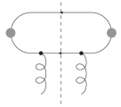
F1

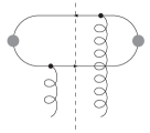
F2

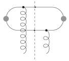
F3

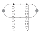
F4

Figure 8: The fermion diagrams for the impact factors.

The first difference is due to the fact that in ${\cal N}=4$ there are 4 Weyl fermions instead of $n_{f}$ Dirac ones. The counting of the number of fields weighted by the right $R$-charge is performed by the trace over the two generators of the $SU_{R}(4)$  group,

$$\operatorname{Tr}_{4}\big{(}T^{A}T^{A}\big{)}=\frac{1}{2}\,,$$ (45)

(there is no sum over $A$ here), taken in the appropriate representation (fundamental for the fermions and vector representation for the scalars).

The chiral nature of the fields introduces additional terms due to a Levi-Civita tensor arising from spinor traces containing a chiral projector. All these terms cancel in the sum of the four diagrams $F1-4$. The complete list of the $\phi_{i}$ is given in the appendix A.2.

The diagrams needed for the computation of the scalar component of the impact factor are depicted in Fig. 9.

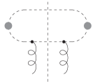
S1

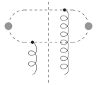
S2

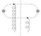
S3

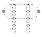
S4

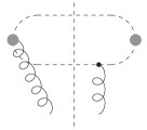
S5

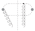
S6

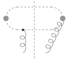
S7

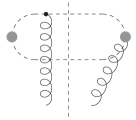
S8

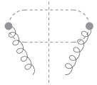
S9

Figure 9: The scalar diagrams for the impact factors.

The trace over the $SU_{R}(4)$  indices now gives

$$\operatorname{Tr}_{6}\big{(}T^{A}T^{A}\big{)}=1\,.$$ (46)

Since the scalars crossing the cut are identical particles there is a symmetry factor $1/2$.

At finite energies, all the diagrams $S1-9$ in Fig. 9 are needed in order to satisfy the Ward identities. At high energies, however, it turns out that the diagrams $S5-9$ are suppressed. As an example, let us consider the diagram $S5$. The gluon polarization tensor is contracted with the polarization vector of the incoming current, which is proportional to $p_{2}$. Then, out of the three parts of the gluon polarization tensor (cf. 11: the index $\rho$ belongs to the upper end of the gluon, $\sigma$ to the lower end):

$$\frac{2p_{2\rho}p_{1\sigma}}{s}+\frac{2p_{1\rho}p_{2\sigma}}{s}+g_{\perp\rho\sigma}\,,$$ (47)

only the second term survives because $p_{2}^{2}=p_{2}^{\mu}g_{\perp\mu\nu}=0$. Note that in the ’normal’ fermionic case it is the first term that gives the leading behavior in the Regge asymptotic. One sees indeed that the contraction of the loop integral numerator with $p_{1}$ provides one power of $s$ less than the leading terms of diagrams $S1-4$. An analogous discussion applies to the contraction of $p_{2}$ with the loop below, and again there is a suppression of a power of $s$. Eventually one sees that a diagram involving $S5$ is $1/s^{2}$ suppressed with respect to the leading term. The same argument applies to the other diagrams $S6-8$, while for $S9$ the suppression is even stronger, $1/s^{4}$, because the same effect takes place for both gluons. We are thus left with the diagrams $S1-4$, which, at high energies, give the full scalar component of the impact factor. The computation mimics closely the fermionic one, and details can be found in appendix A.2.

III.6 The full impact factors

Collecting together all the terms one obtains the full impact factors,

$$\Phi_{A}^{LL^{\prime}aa^{\prime}} = \delta^{aa^{\prime}}\frac{N_{c}\alpha_{s}}{2}Q_{A}Q_{A^{\prime}}\!\!\int_{0}^{1}\!\!d\alpha\!\!\int\!\!\frac{d^{2}\mbox{\boldmath$l$}}{(2\pi)^{2}}\alpha(1-\alpha)$$ (48a)

$$\times\Big{(}\frac{1}{D_{1}}-\frac{1}{D_{2}}\Big{)}\Big{(}\frac{1}{D^{\prime}_{1}}-\frac{1}{D^{\prime}_{2}}\Big{)},$$

$$\Phi_{A}^{Lh^{\prime}aa^{\prime}} = 0\,,$$ (48b)

$$\Phi_{A}^{hh^{\prime}aa^{\prime}} = \delta^{aa^{\prime}}\delta^{hh^{\prime}}\frac{N_{c}\alpha_{s}}{2}\!\!\int_{0}^{1}\!\!d\alpha\!\!\int\!\!\frac{d^{2}\mbox{\boldmath$l$}}{(2\pi)^{2}}$$ (48c)

$$\times\Big{(}\frac{\mbox{\boldmath$N$}_{1}}{D_{1}}-\frac{\mbox{\boldmath$N$}_{2}}{D_{2}}\Big{)}\cdot\Big{(}\frac{\mbox{\boldmath$N$}^{\prime}_{1}}{D^{\prime}_{1}}-\frac{\mbox{\boldmath$N$}^{\prime}_{2}}{D^{\prime}_{2}}\Big{)}\,,$$

with $D_{i}$ and $\mbox{\boldmath$N$}_{i}$ defined by

Comparing (48a-c) with the QCD result of Bartels:2003yj one observes a striking difference: in contrast to the QCD results where helicity conservation holds only in the forward direction, at $t=0$, now for arbitrary $t=-\mbox{\boldmath$q$}^{2}$ all the off-diagonal terms in the polarization indices vanish, as the result of cancellations between the scalar and fermion loops, $\Phi^{\lambda\lambda^{\prime}}\propto\delta^{\lambda\lambda^{\prime}}$. This is a consequence of supersymmetry.

Higher order diagrams with gluon exchange, in the LL approximation, lead to the QCD BFKL Pomeron described in Sec. II.4. This coincidence, at high energies, of nonsupersymmetric Yang-Mills theory and the supersymmetric extension is an artifact of the leading logarithmic approximation, which only depends upon the spin-1 gauge bosons, and not on scalars or fermions. The only place where, in LL, these superpartners appear are the impact factors given now by (48a-c). We have therefore completed our leading logarithmic analysis by proving that the correlation function (III.1) satisfies Regge factorization, and we have computed those buildings blocks which are sensitive to the supersymmetric extension of QCD.

IV Outlook

The AdS/CFT correspondence Maldacena:1997re-Witten:1998qj-Gubser:1998bc conjectures that ${\cal N}=4$ SYM theory is equivalent to Type IIB superstring theory on $AdS_{5}\times S^{5}$. The connection between these apparently different theories is a weak-strong duality: it connects the weak coupling limit of one side with the strong coupling limit on the other side. This opens up the possibility to study aspects of the gauge theory at strong coupling, where traditional tools are unapplicable. In particular, we can address the computation of the $R$-currents correlation function (III.1) in the large $N_{c}$ and large ’t Hooft coupling $\lambda=g_{YM}^{2}N_{c}$ limit. In this limit the relevant string theory is described by the $S^{5}$ compactification of type IIB supergravity in ten dimensions. This reduction gives rise to ${\cal N}=8$, $D=5$ supergravity, with $SO(6)$ Yang-Mills gauge group Schwarz:1983qr ; Pernici:1984xx ; Gunaydin:1984fk ; Kim:1985ez ; Gunaydin:1984qu .

The complete detailed reduction is a problem of great complexity. Fortunately, there exist consistent truncations of the full theory which are much simpler than the full theory. In Cvetic:1999xp it was shown that there is a very simple truncation which contains only a $U(1)$ gauge field and the graviton. Its action reads

$$e^{-1}{\cal L}_{5}=$$ (50)

$$-\frac{1}{2\kappa_{5}^{2}}\Big{(}R+12g^{2}-\frac{1}{4}F^{2}+\frac{1}{12\sqrt{3}}\epsilon^{\mu\nu\rho\sigma\lambda}F_{\mu\nu}F_{\rho\sigma}A_{\lambda}\Big{)}\,.$$

According to the AdS/CFT dictionary, each gauge invariant operator in the gauge theory corresponds to some bulk field in the supergravity theory. The generating functional for the connected correlation functions $W[\zeta]$ of the gauge theory, $\zeta$ being the source for some operator ${\cal O}$, is identified with the on-shell action $S_{\textrm{on-shell}}$ of the gravity theory, with the boundary conditions $\varphi_{(0)}$ for the bulk field $\varphi$ dual to ${\cal O}$ playing the role of its source $\zeta$:

$$W[\varphi_{(0)}]=-S_{\textrm{on-shell}}[\varphi_{(0)}]\,.$$ (51)

The fields dual to the $R$-currents of ${\cal N}=4$ SYM are the gauge fields of the supergravity theory. The truncation (50) contains only one of the 15 gauge fields of the full theory, in the same way as our computation in this paper concerns only one $R$-current of the U(1) subgroup out of the 15 associated with the $SU_{R}(4)$  group. The action (50) is therefore sufficient for the purpose of computing the strong coupling version of our result (48a-c).

The supergravity computation requires the evaluation of the Witten diagrams corresponding to some sources for the gauge field $A_{\mu}$ on the boundary of $AdS_{5}$. Diagrams inferred from the action (50) are depicted in Fig. 10.

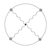
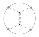
Figure 10: Witten diagrams for the computation of the $R$-current four point function at strong coupling in the truncated theory. The double wavy line in the third graph represents the graviton exchange.

Such computation involves the boundary-to-bulk gauge boson propagator and the bulk-to-bulk propagators for both the gauge field and the graviton. They are well known in the coordinate space D'Hoker:1999jc , and have been extensively used in the past, in order to compute various correlation functions (see for example D'Hoker:1999pj and references therein). Nevertheless the computation of a four point correlation function of $R$-currents is still missing in the literature. We intend to address this computation in the future, not in its full generality but in the Regge limit, where we expect some simplifications to take place.

Returning to the gauge theory side, our analysis of the supersymmetric $R$-current impact factors lays the ground for addressing another aspect of the duality conjecture. Several years ago it has been shown that the BKP evolution equations of $t$-channel states consisting of $n$ Reggeized gluons, in the limit of large $N_{c}$, are integrable Lipatov:1993yb ; LiFK . On the gauge theory side, the four gluon state appears in the high energy limit of the six point correlation function of $R$-currents (in QCD, the analogous process would be the scattering of a virtual photon on two heavy onium states). A study of this correlation function, both on the weak coupling and on the strong coupling side, therefore will allow us to trace the role of this remarkable feature of the Regge limit.

Appendix A

A.1 Sudakov decomposition and polarization vectors

We will work in the frame where $p_{A}$ and $p_{A}^{\prime}$ ($p_{B}$ and $p_{B}^{\prime}$) have a big $+$ ($-$) component, with $p_{\pm}=p_{0}\pm p_{3}$. In this basis the nonvanishing metric coefficients are $g_{+-}=g_{-+}=2$ and $g_{11}=g_{22}=1$, while the Levi-Civita tensor is fully antisymmetric with $\epsilon^{+-12}=-1/2$. In the c.m. we have

$$p_{A}=\Big{(}\sqrt{s},-\frac{Q_{A}^{2}}{\sqrt{s}},0\Big{)}\,,\qquad p_{B}=\Big{(}-\frac{Q_{B}^{2}}{\sqrt{s}},\sqrt{s},0\Big{)}\,.$$ (52)

We use the Sudakov representation for momenta. Let us define the two lightlike (up to ${\cal O}(1/s)$ terms) vectors $p_{1}=p_{A}+x_{A}p_{B}$, $p_{2}=p_{B}+x_{B}p_{A}$ where $x_{A,B}=Q_{A,B}^{2}/2p_{A}\cdot p_{B}$. Then an arbitrary four-momentum $k$ will be decomposed into its projections along $p_{1,2}$ and a transverse component:

$$k=\alpha_{k}p_{1}+\beta_{k}p_{2}+k_{\perp},\qquad\qquad\Big{\{}\begin{array}[]{ccc}\alpha_{k}&=&2p_{2}\cdot k/s\\ \beta_{k}&=&2p_{1}\cdot k/s.\end{array}$$ (53)

The Jacobian is

$$d^{4}k=s/2d\alpha_{k}d\beta_{k}d^{2}\mbox{\boldmath$k$}\,.$$ (54)

The mass-shell conditions for the outgoing momenta fix the longitudinal components of the momentum transferred $q$ to

$$\alpha_{q}=-\frac{Q_{B^{\prime}}^{2}-Q_{B}^{2}+q_{\perp}^{2}}{s}\,,\qquad\qquad\beta_{q}=\frac{Q_{A^{\prime}}^{2}-Q_{A}^{2}+q_{\perp}^{2}}{s}\,,$$ (55)

and the external momenta expressed in Sudakov representation are

$$\begin{array}[]{ll}p_{A}=p_{1}-\frac{Q_{A}^{2}}{s}p_{2}\,,&\qquad p_{A}^{\prime}=p_{1}-\frac{Q_{A^{\prime}}^{2}+q_{\perp}^{2}}{s}p_{2}-q_{\perp}\,,\\ p_{B}=-\frac{Q_{B}^{2}}{s}p_{1}+p_{2}\,,&\qquad p_{B}^{\prime}=-\frac{Q_{B^{\prime}}^{2}+q_{\perp}^{2}}{s}p_{1}+p_{2}+q_{\perp}\,.\end{array}$$ (56)

We now compute the polarization vectors of the external photons. Virtual photons have 3 degrees of freedom, one longitudinal (L) and two transverse ($\pm$) polarizations. The absence of a second longitudinal polarization translates for the amplitude (II) into the constraint (8) provided by gauge invariance. Because of this constraint, the three polarization vectors $\epsilon^{L,\pm}_{\mu}(p)$ represent, for an arbitrary choice of the momentum $p$, a complete basis of the space where the current $j_{\mu}(p)$ belongs to

$$j_{\mu}(p)\in\textrm{Span}\big{\{}\epsilon^{(L,\pm)}_{\mu}(p)\big{\}}\,,$$ (57)

They can be chosen to be orthonormal,

$$\epsilon^{(i)}_{\mu}(p)\epsilon^{(j)\mu}(p)^{*}=-\delta^{ij}\,,$$ (58)

and to satisfy the completeness relation

$$g^{\mu\nu}-\frac{p^{\mu}p^{\nu}}{p^{2}}=\sum_{i=L,\pm}\epsilon^{(i)\mu}(p)\epsilon^{(i)\nu}(p)^{*}\,.$$ (59)

We choose $\epsilon^{L}_{\mu}(p)$ such that its three-dimensional part is proportional to the three-momentum $\vec{p}$ (longitudinal polarization). The two other vectors (helicity $\pm$) are chosen to be transverse. In the Sudakov representation (keeping only the leading term in $s$ for each component) we get

$$\epsilon^{(L)}(p)=$$

$$\quad\frac{i}{Q}\Big{[}\Big{(}\alpha+\frac{2Q^{2}}{s(\alpha+\beta)^{2}}\beta\Big{)}p_{1}+\Big{(}\beta+\frac{2Q^{2}}{s(\alpha+\beta)^{2}}\alpha\Big{)}p_{2}$$

$$\quad+\Big{(}1-\frac{2Q^{2}}{s(\alpha+\beta)^{2}}\Big{)}p_{\perp}\Big{]}\,,$$ (60)

$$\epsilon^{(h)}(p)=\epsilon^{(h)}_{\perp}+\frac{2\epsilon^{(h)}_{\perp}\cdot p}{s(\alpha-\beta)}\Big{(}p_{1}-p_{2}+\frac{p_{\perp}}{\alpha-\beta}\Big{)}\,,$$ (61)

where we have defined

$$\epsilon^{(\pm)}_{\perp}=\frac{1}{\sqrt{2}}(0,1,\pm i,0)\,.$$ (62)

The explicit expressions for the case $p=p_{A},p_{A^{\prime}},p_{B},p_{B^{\prime}}$ can be easily worked out from (56):

$$\epsilon^{(L)}(p_{A}) = \frac{i}{Q_{A}}\Big{(}p_{1}+\frac{Q_{A}^{2}}{s}p_{2}\Big{)}\,,$$ (63)

$$\epsilon^{(L)}(p_{B}) = \frac{i}{Q_{B}}\Big{(}\frac{Q_{B}^{2}}{s}p_{1}+p_{2}\Big{)}\,,$$ (64)

$$\epsilon^{(L)}(p_{A^{\prime}}) = \frac{i}{Q_{A^{\prime}}}\Big{(}p_{1}+\frac{Q_{A^{\prime}}^{2}-q_{\perp}^{2}}{s}p_{2}-q_{\perp}\Big{)},$$ (65)

$$\epsilon^{(L)}(p_{B^{\prime}}) = \frac{i}{Q_{B^{\prime}}}\Big{(}\frac{Q_{B^{\prime}}^{2}-q_{\perp}^{2}}{s}p_{1}+p_{2}+q_{\perp}\Big{)},$$ (66)

$$\epsilon^{(h)}(p_{A,B}) = \epsilon^{(h)}_{\perp}\,,$$ (67)

$$\epsilon^{(h)}(p_{A^{\prime},B^{\prime}}) = \epsilon^{(h)}_{\perp}-\frac{2\epsilon^{(h)}_{\perp}\cdot q}{s}(p_{1}-p_{2}-q_{\perp})\,.$$ (68)

Because of the Ward identities (8) and (22) one is allowed to shift the polarization vectors $\epsilon^{(i)}_{\mu}(p)$ by a four vector proportional to $p$ itself. It is convenient to simplify the polarization vectors as follows:

$$\epsilon^{(L)}(p_{A,A^{\prime}}) = \frac{2Q_{A,A^{\prime}}}{s}p_{2}\,,$$ (69)

$$\epsilon^{(L)}(p_{B,B^{\prime}}) = \frac{2Q_{B,B^{\prime}}}{s}p_{1}\,,$$ (70)

$$\epsilon^{(h)}(p_{A,B}) = \epsilon^{(h)}_{\perp}\,,$$ (71)

$$\epsilon^{(h)}(p_{A^{\prime}}) = \epsilon^{(h)}_{\perp}+\frac{2\epsilon^{(h)}_{\perp}\cdot q}{s}p_{2}\,,$$ (72)

$$\epsilon^{(h)}(p_{B^{\prime}}) = \epsilon^{(h)}_{\perp}-\frac{2\epsilon^{(h)}_{\perp}\cdot q}{s}p_{1}\,.$$ (73)

A.2 Complete list of the $\phi^{ii^{\prime}}_{S,Fl}$

In this appendix we give, for all possible polarizations $\lambda,\lambda^{\prime}=L,\pm$, the full list of the functions $\phi_{i}^{\lambda\lambda^{\prime}}$ for the eight diagrams of Figs. 8 ($i=F1-4$) and 9 ($i=S1-4$). We will make use of the definitions for $D_{i}$ and $N_{i}$, given after (48).

Longitudinal-Longitudinal:

$$\phi_{F1}^{LL^{\prime}} = 2Q_{A}Q_{A^{\prime}}\frac{\alpha^{2}(1-\alpha)^{2}}{D_{1}D^{\prime}_{1}}\,,$$

$$\phi_{F2}^{LL^{\prime}} = -2Q_{A}Q_{A^{\prime}}\frac{\alpha^{2}(1-\alpha)^{2}}{D_{1}D^{\prime}_{2}}\,,$$

$$\phi_{F3}^{LL^{\prime}} = -2Q_{A}Q_{A^{\prime}}\frac{\alpha^{2}(1-\alpha)^{2}}{D_{2}D^{\prime}_{1}}\,,$$

$$\phi_{F4}^{LL^{\prime}} = 2Q_{A}Q_{A^{\prime}}\frac{\alpha^{2}(1-\alpha)^{2}}{D_{2}D^{\prime}_{2}}\,,$$ (74)

$$\phi_{S1}^{LL^{\prime}} = 2Q_{A}Q_{A^{\prime}}\frac{\alpha(1-\alpha)(1/2-\alpha)^{2}}{D_{1}D^{\prime}_{1}}\,,$$

$$\phi_{S2}^{LL^{\prime}} = -2Q_{A}Q_{A^{\prime}}\frac{\alpha(1-\alpha)(1/2-\alpha)^{2}}{D_{1}D^{\prime}_{2}}\,,$$

$$\phi_{S3}^{LL^{\prime}} = -2Q_{A}Q_{A^{\prime}}\frac{\alpha(1-\alpha)(1/2-\alpha)^{2}}{D_{2}D^{\prime}_{1}}\,,$$

$$\phi_{S4}^{LL^{\prime}} = 2Q_{A}Q_{A^{\prime}}\frac{\alpha(1-\alpha)(1/2-\alpha)^{2}}{D_{2}D^{\prime}_{2}}\,.$$ (75)

Longitudinal-Transverse:

$$\phi_{F1}^{Lh^{\prime}} = Q_{A}\frac{\alpha(1-\alpha)(1-2\alpha-h^{\prime}i)}{D_{1}D^{\prime}_{1}}\mbox{\boldmath$N$}^{\prime}_{1}\cdot\mbox{\boldmath$\epsilon$}^{(h^{\prime})*}\,,$$

$$\phi_{F2}^{Lh^{\prime}} = -Q_{A}\frac{\alpha(1-\alpha)(1-2\alpha-h^{\prime}i)}{D_{1}D^{\prime}_{2}}\mbox{\boldmath$N$}^{\prime}_{2}\cdot\mbox{\boldmath$\epsilon$}^{(h^{\prime})*}\,,$$

$$\phi_{F3}^{Lh^{\prime}} = -Q_{A}\frac{\alpha(1-\alpha)(1-2\alpha-h^{\prime}i)}{D_{2}D^{\prime}_{1}}\mbox{\boldmath$N$}^{\prime}_{1}\cdot\mbox{\boldmath$\epsilon$}^{(h^{\prime})*}\,,$$

$$\phi_{F4}^{Lh^{\prime}} = Q_{A}\frac{\alpha(1-\alpha)(1-2\alpha-h^{\prime}i)}{D_{2}D^{\prime}_{2}}\mbox{\boldmath$N$}^{\prime}_{1}\cdot\mbox{\boldmath$\epsilon$}^{(h^{\prime})*}\,,$$ (76)

$$\phi_{S1}^{Lh^{\prime}} = -Q_{A}\frac{\alpha(1-\alpha)(1-2\alpha)}{D_{1}D^{\prime}_{1}}\mbox{\boldmath$N$}^{\prime}_{1}\cdot\mbox{\boldmath$\epsilon$}^{(h^{\prime})*}\,,$$

$$\phi_{S2}^{Lh^{\prime}} = Q_{A}\frac{\alpha(1-\alpha)(1-2\alpha)}{D_{1}D^{\prime}_{2}}\mbox{\boldmath$N$}^{\prime}_{2}\cdot\mbox{\boldmath$\epsilon$}^{(h^{\prime})*}\,,$$

$$\phi_{S3}^{Lh^{\prime}} = Q_{A}\frac{\alpha(1-\alpha)(1-2\alpha)}{D_{2}D^{\prime}_{1}}\mbox{\boldmath$N$}^{\prime}_{1}\cdot\mbox{\boldmath$\epsilon$}^{(h^{\prime})*}\,,$$

$$\phi_{S4}^{Lh^{\prime}} = -Q_{A}\frac{\alpha(1-\alpha)(1-2\alpha)}{D_{2}D^{\prime}_{2}}\mbox{\boldmath$N$}^{\prime}_{2}\cdot\mbox{\boldmath$\epsilon$}^{(h^{\prime})*}\,.$$ (77)

Since under the transformations $\mbox{\boldmath$l$}\rightarrow-\mbox{\boldmath$l$}+\mbox{\boldmath$k$}$ and $\alpha\rightarrow 1-\alpha$, $N_{2}\rightarrow-N_{1}$ and $N^{\prime}_{2}\rightarrow-N^{\prime}_{1}$ in the integrand in (43), the terms proportional to the helicity $h^{\prime}$ in the fermionic parts cancel between $\phi_{F1}^{Lh^{\prime}},\phi_{F4}^{Lh^{\prime}}$ and $\phi_{F2}^{Lh^{\prime}},\phi_{F3}^{Lh^{\prime}}$. The remaining fermionic pieces cancel completely against the corresponding scalar terms.

Transverse-Longitudinal:

$$\phi_{F1}^{hL} = Q_{A^{\prime}}\frac{\alpha(1-\alpha)(1-2\alpha-hi)}{D_{1}D^{\prime}_{1}}\mbox{\boldmath$\epsilon$}^{(h)}\cdot\mbox{\boldmath$N$}_{1}\,,$$

$$\phi_{F2}^{hL} = -Q_{A^{\prime}}\frac{\alpha(1-\alpha)(1-2\alpha-hi)}{D_{1}D^{\prime}_{2}}\mbox{\boldmath$\epsilon$}^{(h)}\cdot\mbox{\boldmath$N$}_{1}\,,$$

$$\phi_{F3}^{hL} = -Q_{A^{\prime}}\frac{\alpha(1-\alpha)(1-2\alpha-hi)}{D_{2}D^{\prime}_{1}}\mbox{\boldmath$\epsilon$}^{(h)}\cdot\mbox{\boldmath$N$}_{2}\,,$$

$$\phi_{F4}^{hL} = Q_{A^{\prime}}\frac{\alpha(1-\alpha)(1-2\alpha-hi)}{D_{2}D^{\prime}_{2}}\mbox{\boldmath$\epsilon$}^{(h)}\cdot\mbox{\boldmath$N$}_{2}\,,$$ (78)

$$\phi_{S1}^{hL} = -Q_{A^{\prime}}\frac{\alpha(1-\alpha)(1-2\alpha)}{D_{1}D^{\prime}_{1}}\mbox{\boldmath$\epsilon$}^{(h)}\cdot\mbox{\boldmath$N$}_{1}\,,$$

$$\phi_{S2}^{hL} = Q_{A^{\prime}}\frac{\alpha(1-\alpha)(1-2\alpha)}{D_{1}D^{\prime}_{2}}\mbox{\boldmath$\epsilon$}^{(h)}\cdot\mbox{\boldmath$N$}_{1}\,,$$

$$\phi_{S3}^{hL} = Q_{A^{\prime}}\frac{\alpha(1-\alpha)(1-2\alpha)}{D_{2}D^{\prime}_{1}}\mbox{\boldmath$\epsilon$}^{(h)}\cdot\mbox{\boldmath$N$}_{2}\,,$$

$$\phi_{S4}^{hL} = -Q_{A^{\prime}}\frac{\alpha(1-\alpha)(1-2\alpha)}{D_{2}D^{\prime}_{2}}\mbox{\boldmath$\epsilon$}^{(h)}\cdot\mbox{\boldmath$N$}_{2}\,.$$ (79)

Here we have the same cancellations as in the longitudinal-transverse case.

Transverse-Transverse:

$$\phi_{F1}^{hh^{\prime}} = \frac{1}{2D_{1}D^{\prime}_{1}}\Big{[}(1-hi\alpha)~{}\mbox{\boldmath$\epsilon$}^{(h)}\cdot\mbox{\boldmath$\epsilon$}^{(h^{\prime})*}~{}\mbox{\boldmath$N$}_{1}\cdot\mbox{\boldmath$N$}^{\prime}_{1}$$

$$+\Big{(}-4\alpha(1-\alpha)+i(h-h^{\prime})(1-\alpha)\Big{)}~{}$$

$$\qquad\qquad\qquad\qquad\qquad\times\mbox{\boldmath$\epsilon$}^{(h)}\cdot\mbox{\boldmath$N$}_{1}~{}\mbox{\boldmath$N$}^{\prime}_{1}\cdot\mbox{\boldmath$\epsilon$}^{(h^{\prime})*}$$

$$-(1-hi\alpha)\Big{(}\mbox{\boldmath$\epsilon$}^{(h)}\cdot\mbox{\boldmath$l$}~{}(1-\alpha)\mbox{\boldmath$q$}\cdot\mbox{\boldmath$\epsilon$}^{(h^{\prime})*}$$

$$\qquad\qquad\qquad\qquad-\mbox{\boldmath$\epsilon$}^{(h)}\cdot(1-\alpha)\mbox{\boldmath$q$}~{}\mbox{\boldmath$l$}\cdot\mbox{\boldmath$\epsilon$}^{(h^{\prime})*}\Big{)}\Big{]}\,,$$

$$\phi_{F2}^{hh^{\prime}} = -\frac{1}{2D_{1}D^{\prime}_{2}}\Big{[}\mbox{\boldmath$\epsilon$}^{(h)}\cdot\mbox{\boldmath$\epsilon$}^{(h^{\prime})*}~{}\mbox{\boldmath$N$}_{1}\cdot\mbox{\boldmath$N$}^{\prime}_{2}$$

$$+\Big{(}-4\alpha(1-\alpha)+i(h-h^{\prime})(1-2\alpha)\Big{)}~{}$$

$$\qquad\qquad\qquad\qquad\qquad\times\mbox{\boldmath$\epsilon$}^{(h)}\cdot\mbox{\boldmath$N$}_{1}~{}\mbox{\boldmath$N$}^{\prime}_{2}\cdot\mbox{\boldmath$\epsilon$}^{(h^{\prime})*}$$

$$-\mbox{\boldmath$\epsilon$}^{(h)}\cdot\mbox{\boldmath$l$}~{}(\mbox{\boldmath$k$}-\alpha\mbox{\boldmath$q$})\cdot\mbox{\boldmath$\epsilon$}^{(h^{\prime})*}$$

$$\qquad\qquad\qquad\qquad+\mbox{\boldmath$\epsilon$}^{(h)}\cdot(\mbox{\boldmath$k$}-\alpha\mbox{\boldmath$q$})~{}\mbox{\boldmath$l$}\cdot\mbox{\boldmath$\epsilon$}^{(h^{\prime})*}\Big{]}\,,$$

$$\phi_{F3}^{hh^{\prime}} = -\frac{1}{2D_{2}D^{\prime}_{1}}\Big{[}\mbox{\boldmath$\epsilon$}^{(h)}\cdot\mbox{\boldmath$\epsilon$}^{(h^{\prime})*}~{}\mbox{\boldmath$N$}_{2}\cdot\mbox{\boldmath$N$}^{\prime}_{1}$$

$$+\Big{(}-4\alpha(1-\alpha)+i(h-h^{\prime})(1-2\alpha)\Big{)}$$

$$\qquad\qquad\qquad\qquad\qquad\times\mbox{\boldmath$\epsilon$}^{(h)}\cdot\mbox{\boldmath$N$}_{2}~{}\mbox{\boldmath$N$}^{\prime}_{1}\cdot\mbox{\boldmath$\epsilon$}^{(h^{\prime})*}$$

$$+\mbox{\boldmath$\epsilon$}^{(h)}\cdot(\mbox{\boldmath$l$}-\mbox{\boldmath$k$})~{}(\mbox{\boldmath$k$}-(1-\alpha)\mbox{\boldmath$q$})\cdot\mbox{\boldmath$\epsilon$}^{(h^{\prime})*}$$

$$\qquad\quad-\mbox{\boldmath$\epsilon$}^{(h)}\cdot(\mbox{\boldmath$k$}-(1-\alpha)\mbox{\boldmath$q$})~{}(\mbox{\boldmath$l$}-\mbox{\boldmath$k$})\cdot\mbox{\boldmath$\epsilon$}^{(h^{\prime})*}\Big{]}\,,$$

$$\phi_{F4}^{hh^{\prime}} = \frac{1}{2D_{2}D^{\prime}_{2}}\Big{[}(1+hi(1-\alpha))~{}\mbox{\boldmath$\epsilon$}^{(h)}\cdot\mbox{\boldmath$\epsilon$}^{(h^{\prime})*}~{}\mbox{\boldmath$N$}_{2}\cdot\mbox{\boldmath$N$}^{\prime}_{2}$$ (80)

$$+\Big{(}-4\alpha(1-\alpha)-i(h-h^{\prime})(1-\alpha)\Big{)}~{}$$

$$\qquad\qquad\qquad\qquad\qquad\times\mbox{\boldmath$\epsilon$}^{(h)}\cdot\mbox{\boldmath$N$}_{2}~{}\mbox{\boldmath$N$}^{\prime}_{2}\cdot\mbox{\boldmath$\epsilon$}^{(h^{\prime})*}$$

$$+(1+hi(1-\alpha))\Big{(}\mbox{\boldmath$\epsilon$}^{(h)}\cdot(\mbox{\boldmath$l$}-\mbox{\boldmath$k$})~{}\alpha\mbox{\boldmath$q$}\cdot\mbox{\boldmath$\epsilon$}^{(h^{\prime})*}$$

$$\qquad\qquad\quad-\mbox{\boldmath$\epsilon$}^{(h)}\cdot\alpha\mbox{\boldmath$q$}~{}(\mbox{\boldmath$l$}-\mbox{\boldmath$k$})\cdot\mbox{\boldmath$\epsilon$}^{(h^{\prime})*}\Big{)}\Big{]}\,,$$

$$\phi_{S1}^{hh^{\prime}} = 2\frac{\alpha(1-\alpha)}{D_{1}D^{\prime}_{1}}\mbox{\boldmath$\epsilon$}^{(h)}\cdot\mbox{\boldmath$N$}_{1}~{}\mbox{\boldmath$N$}^{\prime}_{1}\cdot\mbox{\boldmath$\epsilon$}^{(h^{\prime})*}\,,$$

$$\phi_{S2}^{hh^{\prime}} = -2\frac{\alpha(1-\alpha)}{D_{1}D^{\prime}_{2}}\mbox{\boldmath$\epsilon$}^{(h)}\cdot\mbox{\boldmath$N$}_{1}~{}\mbox{\boldmath$N$}^{\prime}_{2}\cdot\mbox{\boldmath$\epsilon$}^{(h^{\prime})*}\,,$$

$$\phi_{S3}^{hh^{\prime}} = -2\frac{\alpha(1-\alpha)}{D_{2}D^{\prime}_{1}}\mbox{\boldmath$\epsilon$}^{(h)}\cdot\mbox{\boldmath$N$}_{2}~{}\mbox{\boldmath$N$}^{\prime}_{1}\cdot\mbox{\boldmath$\epsilon$}^{(h^{\prime})*}\,,$$

$$\phi_{S4}^{hh^{\prime}} = 2\frac{\alpha(1-\alpha)}{D_{2}D^{\prime}_{2}}\mbox{\boldmath$\epsilon$}^{(h)}\cdot\mbox{\boldmath$N$}_{2}~{}\mbox{\boldmath$N$}^{\prime}_{2}\cdot\mbox{\boldmath$\epsilon$}^{(h^{\prime})*}\,.$$ (81)

Here the cancellations are a bit more involved. In the fermionic sector of each $\phi$, the two terms in the last line cancel each other due to the angular integration in the transverse momenta $l$. In order to see this one combines the two denominators introducing a Feynman parameter and then performs a shift in the $l$ integration. The shift in the numerator cancels between the two terms, and what is left depends upon the angle in the transverse plane only through the $\cos(\theta)$ in the scalar product with the polarization vectors in the numerator; therefore the $\theta$ integral vanishes.

From what is left, all the terms proportional to the helicities $h,h^{\prime}$ cancel in the same way as they did in the previous case: between $\phi_{F1}^{hh^{\prime}},\phi_{F4}^{hh^{\prime}}$ and $\phi_{F2}^{hh^{\prime}},\phi_{F3}^{hh^{\prime}}$ after the change of variable $\mbox{\boldmath$l$}\rightarrow-\mbox{\boldmath$l$}+\mbox{\boldmath$k$}$ and $\alpha\rightarrow 1-\alpha$. Moreover, the terms from the scalar sector cancel exactly with the corresponding terms in the fermionic sector. Eventually only a single term proportional to $\mbox{\boldmath$\epsilon$}^{(h)}\cdot\mbox{\boldmath$\epsilon$}^{(h^{\prime})*}$ is left for each diagram.

References

- (1) V. N. Gribov, Sov. Phys. JETP 26 (1968) 414 [Zh. Eksp. Teor. Fiz. 53 (1967) 654].
- (2) L. N. Lipatov, Phys. Rept. 286 (1997) 131 [arXiv:hep-ph/9610276].
- (3) E. A. Kuraev, L. N. Lipatov and V. S. Fadin, Sov. Phys. JETP 44 (1976) 443 [Zh. Eksp. Teor. Fiz. 71 (1976) 840]; E. A. Kuraev, L. N. Lipatov and V. S. Fadin, Sov. Phys. JETP 45 (1977) 199 [Zh. Eksp. Teor. Fiz. 72 (1977) 377]; I. I. Balitsky and L. N. Lipatov, Sov. J. Nucl. Phys. 28 (1978) 822 [Yad. Fiz. 28 (1978) 1597];
- (4) V. S. Fadin and L. N. Lipatov, Phys. Lett. B 429 (1998) 127 [arXiv:hep-ph/9802290].
- (5) G. Camici and M. Ciafaloni, Phys. Lett. B 412 (1997) 396 [Erratum-ibid. B 417 (1998) 390] [arXiv:hep-ph/9707390]; M. Ciafaloni and G. Camici, Phys. Lett. B 430 (1998) 349 [arXiv:hep-ph/9803389].
- (6) G. Veneziano, Nuovo Cim. A 57 (1968) 190.
- (7) L. N. Lipatov, [arXiv:hep-th/9311037].
-
(8)
L. N. Lipatov,
JETP Lett. 59 (1994) 596;
L. D. Faddeev, G. P. Korchemsky, Phys. Lett. B 342 (1995) 311. -
(9)
J. Bartels,
Nucl. Phys. B 175 (1980) 365;
J. Kwiecinski, M. Praszalowicz, Phys. Lett. B 94 (1980) 413. - (10) J. M. Maldacena, Adv. Theor. Math. Phys. 2 (1998) 231 [Int. J. Theor. Phys. 38 (1999) 1113] [arXiv:hep-th/9711200]; E. Witten, Adv. Theor. Math. Phys. 2 (1998) 253 [arXiv:hep-th/9802150]; S. S. Gubser, I. R. Klebanov and A. M. Polyakov, Phys. Lett. B 428 (1998) 105 [arXiv:hep-th/9802109].
- (11) A. V. Kotikov and L. N. Lipatov, Nucl. Phys. B 582 (2000) 19 [arXiv:hep-ph/0004008]; A. V. Kotikov and L. N. Lipatov, Nucl. Phys. B 661 (2003) 19 [Erratum-ibid. B 685 (2004) 405] [arXiv:hep-ph/0208220]; A. V. Kotikov, L. N. Lipatov and V. N. Velizhanin, Phys. Lett. B 557 (2003) 114 [arXiv:hep-ph/0301021]; A. V. Kotikov, L. N. Lipatov, A. I. Onishchenko and V. N. Velizhanin, Phys. Lett. B 595 (2004) 521 [Erratum-ibid. B 632 (2006) 754] [arXiv:hep-th/0404092].
- (12) R. A. Janik and R. Peschanski, Nucl. Phys. B 565 (2000) 193 [arXiv:hep-th/9907177]; M. Rho, S. J. Sin and I. Zahed, Phys. Lett. B 466 (1999) 199 [arXiv:hep-th/9907126]; R. A. Janik and R. Peschanski, Nucl. Phys. B 586 (2000) 163 [arXiv:hep-th/0003059]; R. A. Janik and R. Peschanski, Nucl. Phys. B 625 (2002) 279 [arXiv:hep-th/0110024]; O. Andreev and W. Siegel, Phys. Rev. D 71 (2005) 086001 [arXiv:hep-th/0410131]; H. Nastase, [arXiv:hep-th/0501039]; R. C. Brower, J. Polchinski, M. J. Strassler and C. I. Tan, [arXiv:hep-th/0603115]; R. C. Brower, M. J. Strassler and C. I. Tan, [arXiv:hep-th/0710.4378]; Y. Hatta, E. Iancu and A. H. Mueller, [arXiv:hep-th/0710.2148]; Y. Hatta, E. Iancu and A. H. Mueller, [arXiv:hep-th/0710.5297].
- (13) J. Bartels, A. De Roeck and H. Lotter, Phys. Lett. B 389 (1996) 742 [arXiv:hep-ph/9608401].
- (14) S. J. Brodsky, F. Hautmann and D. E. Soper, Phys. Rev. D 56 (1997) 6957 [arXiv:hep-ph/9706427].
- (15) S. Caron-Huot, P. Kovtun, G. D. Moore, A. Starinets and L. G. Yaffe, JHEP 0612 (2006) 015 [arXiv:hep-th/0607237].
- (16) G. Chalmers, H. Nastase, K. Schalm and R. Siebelink, Nucl. Phys. B 540 (1999) 247 [arXiv:hep-th/9805105].
- (17) L. Cornalba, M. S. Costa and J. Penedones, [arXiv:hep-th/0801.3002].
- (18) J. Bartels and M. Lublinsky, JHEP 0309 (2003) 076 [arXiv:hep-ph/0308181].
- (19) L. N. Lipatov, Adv. Ser. Direct. High Energy Phys. 5 (1989) 411.
- (20) J. R. Forshaw and D. A. Ross, Cambridge Lect. Notes Phys. 9 (1997) 1.
- (21) L. Brink, J. H. Schwarz and J. Scherk, Nucl. Phys. B 121 (1977) 77.
- (22) V. G. Gorshkov, V. N. Gribov, L. N. Lipatov and G. V. Frolov, Sov. J. Nucl. Phys. 6 (1968) 95 [Yad. Fiz. 6 (1967) 129].
- (23) J. Bartels, K. J. Golec-Biernat and K. Peters, Acta Phys. Polon. B 34 (2003) 3051 [arXiv:hep-ph/0301192].
- (24) J. H. Schwarz, Nucl. Phys. B 226 (1983) 269.
- (25) M. Pernici, K. Pilch and P. van Nieuwenhuizen, Phys. Lett. B 143 (1984) 103.
- (26) M. Gunaydin and N. Marcus, Class. Quant. Grav. 2 (1985) L11.
- (27) H. J. Kim, L. J. Romans and P. van Nieuwenhuizen, Phys. Rev. D 32 (1985) 389.
- (28) M. Gunaydin, L. J. Romans and N. P. Warner, Phys. Lett. B 154 (1985) 268.
- (29) M. Cvetic et al., Nucl. Phys. B 558 (1999) 96 [arXiv:hep-th/9903214].
- (30) E. D’Hoker, D. Z. Freedman, S. D. Mathur, A. Matusis and L. Rastelli, Nucl. Phys. B 562 (1999) 330 [arXiv:hep-th/9902042].
- (31) E. D’Hoker, D. Z. Freedman, S. D. Mathur, A. Matusis and L. Rastelli, Nucl. Phys. B 562 (1999) 353 [arXiv:hep-th/9903196].