Quantum learning by measurement and feedback

Abstract

We investigate an approach to quantum computing in which quantum gate strengths are parametrized by quantum degrees of freedom. The capability of the quantum computer to perform desired tasks is monitored by measurements of the output and gradually improved by successive feedback modifications of the coupling strength parameters. Our proposal only uses information available in an experimental implementation, and is demonstrated with simulations on search and factoring algorithms.

1 Introduction

Quantum information science deals with the use of quantum resources to speed up quantum computing, and to enable new features in quantum communication [1]. The usual paradigm of quantum computing consists of well defined physical storage modes of individual qubits and the existence of a universal set of basic gate operations, from which any unitary operation can be constructed on a full quantum register. The implementation of the universal set of gates in different physical proposals constitutes the back bone for most experimental work on quantum computing. Proof of the ability to perform any computation does not necessarily provide an efficient encoding of the computation in terms of universal gates, and it does not in any simple manner point to optimal performance, e.g., under restrictions set by physically motivated cost functions.

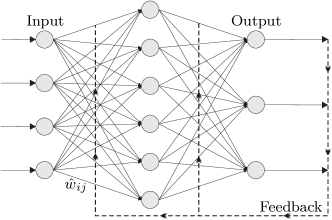
(a)  

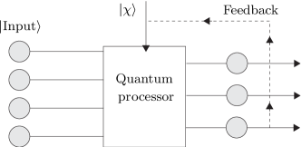
(b)  

Figure 1: Classical (a) and quantum (b) concept of learning by measurement and feedback. The feedback on the dynamics of the system is based upon the examination of the output over many trials. In our quantum learning scenario, quantum measurement back action and unitary feedback operations serve to modify the quantum state $|\chi\rangle$ of the coupling strengths applied in one- and two.-qubit gates in our quantum processor.

In this paper, we present an alternative approach to the programming of a quantum computer based on the neural network paradigm. Neural networks are not programmed from the beginning to accomplish a given task, but instead their coupling parameters (equivalent to the synaptic coupling strengths among neurons in the brain) are being updated according to some policy – often iteratively during a succession of trials according to the successful or failed performance. This adaptive learning, which draws on similarities with the learning of human brains, in the end produces a system, rigged with coupling parameters that enable it to solve the tasks trained. Figure 1(a) shows a model of a neural network with a number of nodes, including input and output nodes, which are connected with coupling strengths, which can be varied according to impulses from external agents who check the output. The success of neural networks as a computational concept relies on the possibility that the resulting circuit is able to successfully solve also new problems of the same kind as the ones trained. For a general reference to neural networks, see [2]. In the neural network, illustrated in part (a) of the figure, both the coupling strengths and the actual physical location of the information are dynamically modified and redistributed during the learning, and one of the strengths of neural networks is precisely the delocalization of the memory which is believed to provide robustness against local damaging effects. The application of a delocalized memory for protection of quantum information in collective local minimum energy states of interacting many-body systems was proposed and analyzed in [3].

In the present paper, we shall focus on the iterative learning aspect of the neural network paradigm. The training of a classical neural network may proceed both via iterative feedback and by single step methods. Our approach is inspired by the iterative version of the artificial neural network paradigm. We shall investigate if this can be implemented in a particularly simple model, where the strengths of the coupling parameters governing a conventional set of universal gates are treated as quantum degrees of freedom, and where a search for optimum values of these parameters is carried out by running the computer many times and acting back on these parameters according to the outcome of the computation. Optimization of quantum algorithm design has been studied, e.g., in [4, 5], where a variational method was applied to identify optimal values of controllable parameters in a Hamiltonian to secure the optimum time evolution of the system density matrix. The work of [4, 5] is connected to the large variety of works on quantum control, applied in particular to femtosecond laser-chemistry where pulse shaping is used to maximize the yield in chemical [6] and biological [7] reactions. Our work differs from the philosophy of [4, 5] by being directed at experimental implementation on a single quantum system. In particular, this implies that complete knowledge of the system wave function or density matrix is not available, and for the design of the feedback loop one has access only to the information extracted by measurements on a single quantum system. By the nature of quantum mechanics, this information is random, and it is an important aspect of the analysis that the control parameters are not only subject to adaptive changes due to the feedback but are also modified by the measurements themselves. We note that pulse shaping in laser chemistry has been successfully implemented in conjunction with experiments, such that the molecules themselves ”are responsible” for solving the Schrödinger equation, and the control fields are subsequently varied according to the experimental output by genetic algorithms [6]. In this case, experiments are carried out on large ensembles of identical systems, thus evading the issues of stochastic measurement outcomes and quantum back action.

The use of learning strategies for quantum computers dedicated to specials tasks, such as pattern recognition, matching of unknown quantum states, and simulation of classical and quantum problems have received some interest [8, 9], and the idea of a classical Hopfield neural network was recently combined with quantum adiabatic computation to implement a novel quantum pattern recognition scheme [10]. In [11], measurements and feedback applied to both the control parameters and to subsequent input states were discussed for the effective solution of a range of special problems. In comparison, our work is more directed towards optimizations of standard quantum computing, and, as exemplified below, the optimal performance of given computational tasks.

2 Controllable one- and two-bit gates

If we implement the neural network with individual two-level quantum systems taking the place of the nodes, and with access to any one- and two-bit operations, the quantum state of the complete system is subject to a time dependent Hamiltonian which can be parametrized with time dependent vectors and matrices $\boldsymbol{w}_{i}$ and $M_{ij}$ of coefficients multiplying operators which are, in turn, expanded on single-qubit Pauli operators $\boldsymbol{\sigma}_{i}$,

$$H=\sum_{i}\boldsymbol{w}_{i}\cdot\boldsymbol{\sigma}_{i}+\sum_{i,j}\boldsymbol{\sigma}_{i}\cdot M_{ij}\boldsymbol{\sigma}_{j}.$$ (1)

In the conventional approach to quantum computing based on sequential application of one and two bit gates, the time dependence of $\boldsymbol{w}_{i}$ and $M_{ij}$ is restricted to non-vanishing values occurring only in discrete intervals.

The success probability of the computational task is a functional of the time dependent coupling strengths $\boldsymbol{w}_{i}(t)$ and $M_{ij}(t)$, and the optimal time dependent Hamiltonian may have no obvious relation to the usual expansion on one and two-qubit gates. We imagine that this approach can be applied to a full implementation of a quantum computer with adjustable coupling strengths, recalling that we deal with only a single realization of the quantum computer, and hence the output of a single run can both be wrong for the best realization of the quantum computer and correct for a very bad one, cf., the finite success probabilities of the Grover and Shor algorithms. Finding the best parameters as quickly as possible thus belongs to the class of stochastic optimization problems, which is a currently very active research field in applied mathematics [12].

In [13], a ”quantum learning machine” is proposed in which control parameters are adjusted according to a feedback mechanism involving the record of failure and success events. We consider in the following a ”full quantum” implementation of such a quantum learning machine in which the $\boldsymbol{w}_{i}$ and $M_{ij}$ are themselves quantum variables, implemented by coupling of our computational qubits to auxiliary quantum systems. A model of such a neural network quantum computer is sketched in Figure 1(b). It shows the quantum processor unit, which transforms an input state into an output state under the action of control parameters supplied by the interaction with the physical system represented by the state $|\chi\rangle$ indicated in the figure. As in the optimal control theory problem, a verification module acts back on the control parameter variables, and by repeated action this system may converge and provide optimum parameters for successful implementation of the quantum processor. In this setup we may thus teach the computer to solve problems that are prohibitively hard to solve but easy to verify classically. Search of unstructured databases, satisfiability problems, factoring, etc., are thus tasks that the successful experimentalist may train the neural quantum computer to master.

The auxiliary quantum system may be quantum fields representing time varying coupling strengths in a quantum manner, but as in optimal control theory we may discretize the time or we may expand the time dependence on a set of time dependent functions and hence represent the coupling strengths with a finite number of degrees of freedom. The interaction with the processing variables should not alter properties of the quantum state $|\chi\rangle$ which may subsequently lead to changes in the control parameters, and the Hamiltonian of the auxiliary system when it is not coupled to the processor must commute with the observables representing the coupling strengths, i.e. the coefficients $\boldsymbol{w}_{i}$ and $M_{ij}$ must be Quantum Non-Demolition (QND) observables. The logical state $|1\rangle$ population in the control bit in a two-bit control-not or a three-bit control-control-not operation is an example of such a (discrete) implementation of $w$ and $M$ components. The auxiliary system may of course be physically equivalent with the processing system, and e.g., part of the ions in an ion string, using for example the approach in [14] to implement multi-qubit gates. The idea put forth in this paper is theoretical and conceptual, and should indeed be applicable to any physical implementation of a quantum computer. In the following we will discuss the idea formally and independently of any specific physical system.

3 Measurement back action and feedback on control parameters

We are now ready to propose a procedure, where a circuit with register qubits which are coupled to a number of auxiliary quantum systems is allowed to propagate a given input. The resulting state of the register is read out by a projective measurement, and depending on the quality of the output, the experimental procedure consists in applying a feedback to the control parameter components of the system, and then repeat the computational step with the same or with other relevant input states. After many trials, the experimentalist should have a quantum computer at her disposal which has been trained without any need for theoretical solutions of the time evolution problem or knowledge about the quantum state of the control parameters produced by the protocol.

In our proof-of-concept, we will focus in the following on the very restricted case of a single one-dimensional control parameter with continuous real spectrum. We thus operate with a single parameter $\phi$ which controls a certain interaction in the quantum circuit instead of addressing a full neural network problem with a large number of adaptive parameters. This simple model enables the study of the time evolution described by a parametrized family of unitary operators $U(\phi)$.

The action of the Hamiltonian on the coupling parameter and quantum processor product Hilbert space is given by

$$U_{\mathrm{tot}}=\int\!\mathrm{d}{\phi}\ \!|\phi\rangle\langle\phi|\otimes U(\phi)$$ (2)

and it produces an entangled state with correlations between the parameter eigenkets $|\phi\rangle$ and the result of the algorithm $U(\phi)|\textrm{input}\rangle$. After a projective measurement on the output state $|r\rangle$, with probability $P(r)=\int\!\mathrm{d}{\phi}\ \!\left|\chi(\phi)\right|^{2}\left|\langle r|U(\phi)|\textrm{input}\rangle\right|^{2}$, the joint state becomes $\int\!\mathrm{d}{\phi}\ \!\chi(\phi)\langle r|U(\phi)|\textrm{input}\rangle|\phi\rangle\otimes|r\rangle/\sqrt{P(r)}$.

The register is no longer entangled with the parameter-system, and the coupling parameter wave function has been updated according to

$$\chi(\phi)\longrightarrow\chi(\phi)\langle r|U(\phi)|\textrm{input}\rangle/\sqrt{P(r)}.$$ (3)

The function $\phi\mapsto\left|\langle r|U(\phi)|\textrm{input}\rangle\right|^{2}$ is a ”filter”, peaked around the values of $\phi$ which produce the result $|r\rangle$ with high probability. Measurements of the register in state $|r\rangle$ hence enhance the value of the posterior wave function $\chi(\phi)$ around these values, and if we are lucky and measure only output states $|r\rangle$ which pass the verification test, the quantum state of the auxiliary system thus, by itself, converges towards the optimal parameters. When we obtain results that do not pass the test, however, the measurement process will reduce the probability in the optimal regions of the parameter state, and a suitable active feedback strategy must be applied.

We note that the optimal performance of the protocol may be obtained for a narrow interval of the $\phi$ parameters, but although the current wave function $\chi(\phi)$ may be peaked in this interval, we may still obtain a negative outcome due to the non-unit success probability of even the optimum quantum algorithm. We should hence also make an attempt to counteract the erroneous reduction of the wave function in regions with high success probability.

From a theorist’s perspective, one may well imagine an analysis of the states and operations involved, leading to a good feedback strategy, but we emphasize, that we are here investigating a scheme that is supposed to work without such extra specific knowledge. We shall therefore only apply ”natural” and quite conservative feedback ideas. We have successfully tried push operations, where we displace the $\phi$ argument alternatively to the left and right at every negative outcome of the verification step, decreasing gradually the magnitude of the push by the inverse of the square root of the number of successful outcomes. This has the effects of smoothing out dips stemming from negative outcomes. Rather than stepping alternatively to the left and right, we have also applied ideas from quantum walks [15] in $\phi$-space, where we, after a measurement with erroneous outcome, split the $\phi$ eigenkets coherently towards both lower and higher arguments. This is for example done using a Hamiltonian specified by $H|\phi\rangle=\lambda(|\phi+\delta\phi\rangle+|\phi-\delta\phi\rangle)$, which after a time $\delta t$ leads to the unitary feedback evolution operator

$$U_{\textrm{fb}}=p_{0}(x)\mathds{1}+\sum_{l=1}^{\infty}p_{l}(x)\!\left(\mathscr{T}(l\delta\phi)+\mathscr{T}(-l\delta\phi)\right),$$ (4)

where $x=\lambda\delta t/\hbar$, $p_{l}(x)=\sum_{j=l}^{\infty}(-ix)^{2j-l}/(j!(j-l)!)$ and $\mathscr{T}(\Delta x)$ is the translation operator of distance $\Delta x$. The functions $p_{l}(x)$ are complex, and we have found it beneficial to counter the build-up of undesired interference effects produced by the phases of $p_{l}(x)$ by applying a pseudo-random dephasing over the parameter register.

We may design the protocol so that the initial wave function $\chi(\phi)$ is real and almost uniform until the first iteration outcome, which is most likely to be erroneous. The state after this measurement thus attains a dip rather than a peak at the optimum value of the coupling parameter, and to significantly improve the state, we can simply apply a single step of the Grover inversion about the mean operation on the control parameter system [16]. This feedback operation thus converts the unwanted dip into a peak at the optimum $\phi$ value. Due to generally complex and nonuniform amplitudes, the future evolution unfortunately does not benefit from further application of this operation, but it gets us going in the right direction, and we henceforth proceed with feedback actions, pushing the control parameter more gently in response to erroneous outcomes.

4 Numerical examples

We will now present results of our numerical simulations of the training of a quantum circuit to perform the Grover search algorithm and the Shor factoring algorithm. The simulations were carried out on a classical computer and using random number generators to simulate the random outcome of measurements on the quantum system. We emphasize that although the simulations proceeded by evolution of the full quantum state, all steps in our protocol are designed to be carried out in an experimental implementation with access only to the sequence of right and wrong answers by the quantum processor.

4.1 Application to Grover’s search algorithm

The generalized Grover or amplitude amplification algorithm [17], can rotate a given source state $|s\rangle$ close to a target state $|t\rangle$ using any unitary transformation $V$ in no more than $1/\left|V_{ts}\right|$ steps, where $\langle t|V|s\rangle=V_{ts}\neq 0$. The algorithm uses operations that change the sign of the $|s\rangle$ and $|t\rangle$ amplitudes [16], and using for the initial state $|s\rangle$ an equal superposition of all $N_{el}$ classical computational states we get the original Grover algorithm with $V_{ts}=1/\sqrt{N_{el}}$.

We have in our numerical study simulated a computer which, instead of the change of sign on the target state has been programmed to implement an arbitrary phase-shift i.e. $|t\rangle\to e^{i\phi}|t\rangle$ instead of $|t\rangle\to-|t\rangle$, and we watch the adaptive modification of the state $\chi(\phi)$ representing an initially unknown phase shift towards a state with a well defined, optimum, phase shift.

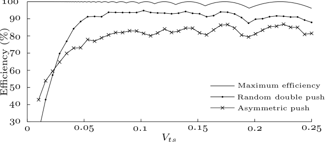
Figure 2: Average performance of Grover algorithm adaptively trained by single-push and double-push feedback. Results are shown after only $120$ iterations of the algorithm. The upper curve shows the maximal success probability of the usual Grover search algorithm. The size of the search space is given as $1/V_{ts}^{2}$, that is from $10000$ to $16$ elements.

Figure 3: Average evolution of the success probability of the system trained with the single-push (dashed) and double-push (solid) feedback for $V_{ts}\approx$0.07$$ corresponding to the search of a database with $\sim$ 200 elements. Inset: The variance of the $\left|\chi\right|^{2}$-distribution as a function of iteration number.

Figure 4: $10\text{\,}\%$ and $25\text{\,}\%$ quantiles of the number of iterations needed to obtain a probability of success of $95\text{\,}\%$ of the theoretical maximum. The data show that with the asymmetric push feedback, a near-optimal Grover search on databases with up to $10000$ elements can be taught in less than 20 iterations in the best $10\text{\,}\%$ runs, while 10-12 iterations suffice for smaller databases where success is achieved in $25\text{\,}\%$ of the runs.

Figure 2 shows the efficiency of the adaptive learning applied to the Grover algorithm, defined as the average success-probability obtained by an ensemble of computers that have been trained by a mere $120$ iterations. The efficiency is shown as a function of $V_{ts}=1/\sqrt{N_{el}}$, corresponding to the search of registers with a few to several thousand elements. The lower curves in the plot refer to the simple push strategy with decreasing magnitude and the double push, or quantum walk, strategy followed by a randomization of the phase. The double push methods work with high success probability in a wide interval, but both methods degrade for large search problems with very small $V_{ts}$. For large $V_{ts}$, i.e., for small registers, the Grover algorithm is not always $100\text{\,}\%$ efficient, which naturally causes the teaching algorithms to produce worse results. The upper curve in figure 2 thus indicates the success probability of the conventional Grover algorithm at different $V_{ts}$. Our simulated curves do not reach this optimum, because they represent an average, including contributions from entirely unsuccessful teaching attempts. Such unsuccessful attempts are the ones, where no tendency of improved success is observed in the measurement read-out, and such runs of the learning algorithm would typically be discarded in an experimental implementation of the scheme.

In Fig.3 the quality of the algorithm is plotted as a function of the number of iterations, and the insert shows the variance of the parameter $\phi$ according to the distributions $|\chi(\phi)|^{2}$ found in several runs of the protocol. After $100$ iterations the learning saturates and any further increase in quality becomes more or less negligible.

Note that the variance of $\left|\chi(\phi)\right|^{2}$ is not a quantity that we assume available, or for that sake, of relevance in an implementation of our proposal. The plot only shows that $\phi$ localizes with the application of our feedback scheme.

A different representation of the simulation data can be seen in figure 4, where we show the required number of iterations where at least $10\text{\,}\%$ ($25\text{\,}\%$) of our simulations have led to a performance better than $95\text{\,}\%$ of the theoretical maximum. Thus for a wide range of register sites only about $10$-$20$ iterations are needed for the $25\text{\,}\%$ best runs to reach $95\text{\,}\%$ of the maximum success probability.

4.2 Application to Shor’s factoring algorithm

We have also applied the learning algorithm to the discrete Fourier transform which is an essential part of the Shor factoring algorithm. The discrete Fourier transform implements controlled phase shifts $\phi_{m}=\pi/2^{m}$, falling off with the separation $m$ between the qubit register positions in a binary representation of integers. It has been proposed, in order to gain speed and to reduce the effects of decoherence and noise [18], to implement an approximate Fourier transform, which only considers couplings up to a given maximum distance. If the gates are thus truncated, one may well speculate that other phases than the usual choice leads to better performance. This is verified by numerical computations showing an efficiency-gain of up to $12\text{\,}\%$ depending on the degree of approximation. For example a quantum Fourier transform of $14$ qubits with nearest neighbor couplings could be improved $12.3\text{\,}\%$ just by chosing apropriate phases. See Table 1 for more examples. Although the identification of optimum phases seems to converge well on not too large systems, the problem constitutes a good example of our aims to find optimum parameters in a quantum processor by measurements and feedback. We have thus treated the unknown phase(s) as provided by an auxiliary quantum system and applied the same feedback algorithm as described above in order to teach a Fourier transform network with freedom in the choice of phases to solve its task optimally.

		Separation, $m$
		1	2	3
Qubits	6	$4.5$	$1.3$
	8	$7.3$	$3.2$	$0.5$
	10	$10.5$	$6.0$	$1.2$
	12	$11.7$	$7.5$	$2.1$
	14	$12.3$	$11.4$	$3.0$

Table 1: Improvement in percent of approximate quantum Fourier transform by use of non-standard phases on registers with different numbers of qubits and with truncation of two-qubit gates at separations 1, 2 and 3.

Fig. 5(a) shows the results of using the asymmetric push algorithm on the approximate quantum Fourier transform with nearest neighbor coupling ($m=1$) as described in [18]. After $120$ iterations on a number of independent trials, we end up with different states of the control parameter and, hence, with different success probabilities in the subsequent performance of the computation. The shading in the figure indicates for different sizes of the register between 6 and 17 qubits the fraction of events with success probabilities in 2.5 % wide intervals. For comparison, the solid curve in the plot shows the average efficiency, while the dotted line indicates the average success probability using standard phases.

The 90 % quantile (the dash-dotted line) shows the success probability delimiting the 10 % best from the 90 % worst performances and show that a significant fraction of runs result in very good performance. These particularly successful runs can, to some extent, be identified by the experimenter through a larger number of successful outcomes of the verification in the 120 iterations. The dashed line in the figure shows the theoretical maximum success probability, which we calculated by using standard optimization algorithms. As shown in the figure, the 90% quantile lies very close to this maximum, indicating that 10% of the parameters found by our neural learning approach are very close to optimal.

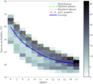
(a)  

(b)  

Figure 5: Distribution of the success-probability of the test-runs (a) for nearest neighbor couplings and (b) for nearest and next-nearest neighbor couplings. The shading shows how large a fraction of our test runs have success probability within different 2.5 % wide percent intervals after 120 iterations for 6 to 17 qubits. The solid curve indicates the average success probability and the dash-dotted curve shows the 90% quantile. The dotted and dashed line shows the average success probability for standard and optimal phases respectively.

We have also attempted to optimize the $m=2$-case, i.e. a problem with two unknown parameters, and an algorithm producing viable solutions was found, but the probability of success was not as illustrative as the cases presented for the $m=1$ case (see figure 5(b)) . This we ascribe to the higher dimensionality of the problem, and it is clearly a challenge for any feedback strategy to apply appropriate corrections to multi-dimensional control parameters.

5 Conclusion

In conclusion, we have proposed to treat coupling strengths in a quantum circuit as quantum variables and to apply feedback strategies on these variables to adaptively teach the circuit to solve given tasks. The proposal is formulated such that it may be implemented in a suitable experimental set-up, and such that there is no need for an elaborate parallel theoretical calculation. One- and two-parameter simulations confirm the viability of the proposal, but it should be recalled that with the extension to many coupling parameters, the optimum feedback in the corresponding multi-dimensional parameter space is highly non-trivial. In the latter case, solutions may be found which rely on superposition states or perhaps entangled states of the coupling parameter systems, and in such cases the algorithm optimization goes far beyond optimum classical solutions for the control parameters in Eq. (1). It should be emphasized that the applied feedback strategies have been quite simple and general, and that the resulting performance is both remarkable and encouraging. For physical implementation, we note that the coupling parameter variables can be incorporated on equal footing with the register qubits of the quantum computer, but they should be restricted to QND behavior, and they should be easy to address by the feedback. In a longer perspective our proposal may open the possibility to identify optimum devices for few bit operations such as operations within error correcting codes [19, 20] and for the training of a many qubit ”quantum brain”, that accomplishes very difficult tasks.

References

- [1] M. A. Nielsen and I. L. Chuang. Quantum Computation and Quantum Information. Cambridge University Press, 2000.
- [2] J. Hertz, R. G. Palmer, and A. Krogh. Introduction to the Theory of Neural Computation. Addison Wesley, 1991.
- [3] M. Pons, V. Ahufinger, C. Wunderlich, A. Sanpera, S. Braungardt, A. Sen(De), U. Sen, and M. Lewenstein. Trapped ion chain as a neural network: Error resistant quantum computation. Phys. Rev. Lett., 98(2):023003, Jan 2007.
- [4] E. C. Behrman, J. E. Steck, P. Kumar, and K. A. Walsh. Quantum algorithm design using dynamic learning. Quantum Information and Computation, 8:12, 2008.
- [5] N. Khaneja, R. Brockett, and S.0 J. Glaser. Time optimal control in spin systems. Phys. Rev. A, 63(3):032308, Feb 2001.
- [6] T. Brixner, N. H. Damrauer, P. Niklaus, and G. Gerber. Photoselective adaptive femtosecond quantum control in the liquid phase. Nature, 414:57–60, November 2001.
- [7] J. L. Herek, W. Wohlleben, R. J. Cogdell, D. Zeidler, and M. Motzkus. Quantum control of energy flow in light harvesting. Nature, 417:533–535, May 2002.
- [8] A. Atici and R.A. Servedio. Improved Bounds on Quantum Learning Algorithms. Quantum Information Processing, 4(5):355–386, 2005.
- [9] M. Sasaki and A. Carlini. Quantum learning and universal quantum matching machine. Phys. Rev. A, 66(2):22303, 2002.
- [10] R. Neigovzen, J. Neves, R. Sollacher, and S. J. Glaser. Quantum pattern recognition with liquid state nmr. arxiv: 0802.1592, February 2008.
- [11] M. Zak. Quantum Analog Computing. Chaos, Solitons and Fractals, 10(10):1583–1620, 1999.
- [12] S. Asmussen and P.W. Glynn. Stochastic simulation: algorithms and analysis. Springer, New York, 2007.
- [13] J. Bang, J. Lim, MS Kim, and J. Lee. Quantum Learning Machine. arXiv:0803.2976, 2008.
- [14] X. Wang, A. Sørensen, and K. Mølmer. Multibit gates for quantum computing. Phys. Rev. Lett., 86:3907, April 2001.
- [15] V. M. Kendon. A random walk approach to quantum algorithms. Phil Trans Roy Soc A, 364(1849):3407–3422, Dec 2006.
- [16] L. K. Grover. A fast quantum mechanical algorithm for database search. In STOC ’96: Proc. 28. Ann. ACM symp on theory of computing, pages 212–219, New York, USA, 1996. ACM.
- [17] L. K. Grover. Quantum computers can search rapidly by using almost any transformation. Phys. Rev. Lett., 80(19):4329–4332, May 1998.
- [18] A. Barenco, A. Ekert, K Suominen, and P. Törmä. Approximate quantum fourier transform and decoherence. Phys. Rev. A, 54(1):139–146, Jul 1996.
- [19] A. M. Steane. Error correcting codes in quantum theory. Phys. Rev. Lett., 77(5):793–797, Jul 1996.
- [20] P. Shor. Scheme for reducing decoherence in quantum computer memory. Phys. Rev. A, 52(4):R2493–R2496, Oct 1995.