The ground state energy at unitarity
Abstract
We consider two-component fermions on the lattice in the unitarity limit. This is an idealized limit of attractive fermions where the range of the interaction is zero and the scattering length is infinite. Using Euclidean time projection, we compute the ground state energy using four computationally different but physically identical auxiliary-field methods. The best performance is obtained using a bounded continuous auxiliary field and a non-local updating algorithm called hybrid Monte Carlo. With this method we calculate results for and fermions at lattice volumes and extrapolate to the continuum limit. For fermions in a periodic cube, the ground state energy is times the ground state energy for non-interacting fermions. For fermions the ratio is .
pacs:
03.75.Ss, 05.30.Fk, 21.65.+f, 71.10.Fd, 71.10.HfI Introduction
The unitarity limit describes attractive two-component fermions in an idealized limit where the range of the interaction is zero and the scattering length is infinite. The name refers to the fact that the S-wave cross section saturates the limit imposed by unitarity, , for low momenta . In the unitarity limit details about the microscopic interaction are lost, and the system displays universal properties. Throughout our discussion we refer to the two degenerate components as up and down spins, though the correspondence with actual spin is not necessary. At sufficiently low temperatures the spin-unpolarized system is believed to be superfluid with properties in between a Bardeen-Cooper-Schrieffer (BCS) fermionic superfluid at weak coupling and a Bose-Einstein condensate of dimers at strong coupling Eagles (1969); Leggett (1980); Nozieres and Schmitt-Rink (1985).
In nuclear physics the phenomenology of the unitarity limit is relevant to cold dilute neutron matter. The scattering length for elastic neutron-neutron collisions is about fm while the range of the interaction is comparable to the Compton wavelength of the pion, fm. Therefore the unitarity limit is approximately realized when the interparticle spacing is about fm. While these conditions cannot be produced experimentally, neutrons at around this density may be present in the inner crust of neutron stars Pethick and Ravenhall (1995); Lattimer and Prakash (2004).
The unitarity limit has been experimentally realized with cold atomic Fermi gases. For alkali atoms the relevant length scale for the interatomic potential at long distances is the van der Waals length . If the spacing between atoms is much larger than , then to a good approximation the interatomic potential is equivalent to a zero range interaction. The scattering length can be manipulated using a magnetic Feshbach resonance O’Hara et al. (2002); Gupta et al. (2003); Regal and Jin (2003); Bourdel et al. (2003); Gehm et al. (2003); Bartenstein et al. (2004); Kinast et al. (2005). This technique involves a molecular bound state in a “closed” hyperfine channel crossing the scattering threshold of an “open” channel. The magnetic moments for the two channels are typically different, and so the crossing can be produced using an applied magnetic field.
At zero temperature there are no dimensionful parameters other than particle density. For up spins and down spins in a given volume we write the energy of the unitarity-limit ground state as . For the same volume we call the energy of the free non-interacting ground state , and the dimensionless ratio of the two ,
| (1) |
The parameter is defined as the thermodynamic limit for the spin-unpolarized system,
| (2) |
Several experiments have measured from the expansion of 6Li and 40K released from a harmonic trap. Some recent measured values for are Kinast et al. (2005), Stewart et al. (2006), and Bartenstein et al. (2004). The disagreement between these measurements and larger values for reported in earlier experiments O’Hara et al. (2002); Bourdel et al. (2003); Gehm et al. (2003) suggest further work may be needed.
There are numerous analytic calculations of using a variety of techniques such as BCS saddle point and variational approximations, Padé approximations, mean field theory, density functional theory, exact renormalization group, dimensional -expansions, and large- expansions Engelbrecht et al. (1997); Baker (1999); Heiselberg (2001); Perali et al. (2004); Schäfer et al. (2005); Papenbrock (2005); Nishida and Son (2006, 2007); Chen (2007); Krippa (2007); Arnold et al. (2007); Nikolic and Sachdev (2007); Veillette et al. (2007). The values for range from to . Fixed-node Green’s function Monte Carlo simulations for a periodic cube have found to be for Carlson et al. (2003) and for larger Astrakharchik et al. (2004); Carlson and Reddy (2005). A restricted path integral Monte Carlo calculation finds similar results Akkineni et al. (2006), and a sign-restricted mean field lattice calculation yields Juillet (2007).
There have also been simulations of two-component fermions on the lattice in the unitarity limit at nonzero temperature. When data are extrapolated to zero temperature the results of Bulgac et al. (2006, 2008) produce a value for similar to the fixed-node results. The same is true for Burovski et al. (2006a, b), though with significant error bars. The extrapolated zero temperature lattice results from Lee and Schäfer (2006a, b) established a bound, , while more recent lattice calculations yield Abe and Seki (2007a, b). The work of Abe and Seki (2007a, b) includes a comparison of two lattice algorithms similar to the ones discussed in this paper.
In Lee (2006a) was calculated on the lattice using Euclidean time projection for and lattice volumes . From these small volumes it was estimated that . More recent results using a technique called the symmetric heavy-light ansatz found similar values for at the same lattice volumes and estimated in the continuum and thermodynamic limits Lee (2008).
For lattice calculations of at fixed , systematic errors due to nonzero lattice spacing can be removed by extrapolating to the continuum limit. At unitarity where the scattering length is set to infinity, this continuum extrapolation corresponds with increasing the lattice volume as measured in lattice units. In this paper we present new lattice results using the Euclidean time projection method introduced in Lee (2006a) and extrapolate to the continuum limit.
In earlier work Lee (2006a, 2007) singular matrices were encountered that prevented calculations at larger volumes. We discuss this and related issues by considering four different auxiliary-field methods which reproduce exactly the same Euclidean lattice model. These four methods include a Gaussian-integral auxiliary field, an exponentially-coupled auxiliary field, a discrete auxiliary field, and a bounded continuous auxiliary field. By far the best performance is obtained using the bounded continuous auxiliary field and hybrid Monte Carlo Duane et al. (1987). With this method we calculate the ground state energy for and fermions at lattice volumes and extrapolate to the continuum limit.
II Euclidean time lattice formalism
Throughout our discussion of the lattice formalism we use dimensionless parameters and operators corresponding with physical values multiplied by the appropriate power of the spatial lattice spacing . In our notation the three-component integer vector labels the lattice sites of a three-dimensional periodic lattice with dimensions . The spatial lattice unit vectors are denoted , , . We use to label lattice steps in the temporal direction. denotes the total number of lattice time steps. The temporal lattice spacing is given by , and is the ratio of the temporal to spatial lattice spacing. We also define , where is the fermion mass in lattice units.
We discuss four different formulations of the Euclidean time lattice for interacting fermions: Grassmann path integrals with and without auxiliary field and transfer matrix operators with and without auxiliary field. For any spatial and temporal lattice spacings these four formulations produce exactly the same physics, as indicated in Fig. 1. We follow the order of discussion indicated by the numbered arrows in Fig. 1.

II.1 Grassmann path integral without auxiliary field
Let and be anticommuting Grassmann fields for spin . The Grassmann fields are periodic with respect to the spatial lengths of the lattice,
| (3) |
and antiperiodic along the temporal direction,
| (4) |
We write as shorthand for the integral measure,
| (5) |
The Grassmann spin densities, and are defined as
| (6) |
| (7) |
We consider the Grassmann path integral
| (8) |
| (9) |
The action consists of the free fermion action
| (10) |
and an attractive contact interaction between up and down spins. We take this action as the definition of the lattice model. All other formulations introduced later will be shown to be exactly equivalent.
We use a fermion mass of MeV and lattice spacings MeV, MeV. In dimensionless lattice units the corresponding parameters are and . These are the same values used in Lee (2006a) and is motived by the relevant physical scales for dilute neutron matter.
II.2 Interaction coefficient for general spatial and temporal lattice spacings
We use Lüscher’s formula Lüscher (1986); Beane et al. (2004); Seki and van Kolck (2006); Borasoy et al. (2007a) to relate the coefficient to the S-wave scattering length. We consider one up-spin particle and one down-spin particle in a periodic cube of length . Lüscher’s formula relates the two-particle energy levels in the center-of-mass frame to the S-wave phase shift,
| (11) |
where is the three-dimensional zeta function,
| (12) |
For small momenta the effective range expansion gives
| (13) |
where is the scattering length and is the effective range.
In terms of , the energy of the two-particle scattering state is
| (14) |
We compute the location of the two-particle scattering pole by summing the bubble diagrams shown in Fig. 2.
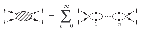
After writing the sum of bubble diagrams as a geometric series, the relation between and becomes
| (15) |
where
| (16) |
These expressions were first derived in Lee and Schäfer (2005). In the unitarity limit the scattering length is set to infinity and all other effective range parameters are set to zero. From Eq. (13) and (11) this is equivalent to setting . To minimize lattice discretization errors we pick the root of closest to zero, . After selecting some large value for , we use Eq. (14) and (15) to determine the unitarity limit value for the coefficient . For our chosen lattice parameters is MeV-2 in physical units or in dimensionless lattice units.
II.3 Transfer matrix operator without auxiliary field
We convert the Grassmann path integral into the trace of a product of transfer matrix operators using the exact correspondence Creutz (1988, 2000)
| (17) |
where We use and to denote fermion annihilation and creation operators respectively for spin at lattice site . The symbols in (17) indicate normal ordering. Let us define
| (18) |
and
| (19) |
| (20) |
Then
| (21) |
where is the normal-ordered transfer matrix operator
| (22) |
II.4 Grassmann path integral with auxiliary field
We consider four different auxiliary-field transformations labelled with the subscript . Let us define the Grassmann actions
| (23) |
and Grassmann path integrals
| (24) |
where is a real-valued function over all lattice sites. For , we use a Gaussian-integral transformation similar to the original Hubbard-Stratonovich transformation Stratonovich (1958); Hubbard (1959),
| (25) |
| (26) |
For we use an auxiliary field with exponential coupling to the fermion densities,
| (27) |
| (28) |
This is the auxiliary-field transformation used in Lee and Schäfer (2005, 2006a, 2006b); Lee (2006a, 2007). For we use a discrete auxiliary field taking values or at each lattice site,
| (29) |
| (30) |
The discrete Hubbard-Stratonovich transformation was first introduced by Hirsch in Hirsch (1983) and has been used in a number of recent lattice simulations Bulgac et al. (2006); Lee (2006b); Abe and Seki (2007a, b); Bulgac et al. (2008). For we introduce a new transformation which uses a bounded but continuous auxiliary field,
| (31) |
| (32) |
The motivation for the new transformation is discussed later when comparing and analyzing computational performance.
For each the integral transformations are defined so that
| (33) |
| (34) |
Since all even products of Grassmann variables commute, we can factor out the term in involving the auxiliary field at . To shorten the notation we temporarily omit writing explicitly. For each we find
| (35) |
For the four cases the integral of is
| (36) |
| (37) |
| (38) |
| (39) |
Therefore
| (40) |
when the interaction coefficients satisfy
| (41) |
III Transfer matrix operator with auxiliary field
Using Eq. (17) and (40) we can write as a product of transfer matrix operators which depend on the auxiliary fields,
| (42) |
where
| (43) |
For the numerical lattice calculations presented in this paper we use the auxiliary-field transfer matrix operators in Eq. (43).
Let be the normalized Slater-determinant ground state on the lattice for a non-interacting system of up spins and down spins. For each spin we fill momentum states in the order shown in Table 1.
| additional momenta filled | |
|---|---|
We construct the Euclidean time projection amplitude
| (44) |
where . The result upon integration gives the same for each
As a result of normal ordering, consists of only single-particle operators interacting with the background auxiliary field and no direct interactions between particles. We find
| (45) |
where
| (46) |
for matrix indices . are single-particle momentum states comprising the Slater-determinant initial/final state. The single-particle interactions in are the same for both up and down spins, and this is why the determinant in Eq. (45) is squared. Since the matrix is real-valued, the square of the determinant is nonnegative and there is no problem with oscillating signs.
For the interacting lattice system at unitarity, we label the energy eigenstates with energies in order of increasing energy,
| (47) |
In the transfer matrix formalism these energies are defined in terms of the logarithm of the transfer matrix eigenvalue,
| (48) |
Let us define as the inner product with the initial free fermion ground state,
| (49) |
In the following we assume that , the overlap between free fermion ground state and the interacting ground state, is nonzero.
Let us define a transient energy expectation value that depends on the Euclidean time
| (50) |
The spectral decomposition of gives
| (51) |
and at large Euclidean time significant contributions come from only low energy eigenstates. For large we find
| (52) |
For low energy excitations is much smaller than the energy cutoff scale imposed by the temporal lattice spacing. Therefore
| (53) |
The ground state energy is given by the limit
| (54) |
IV Importance sampling
We calculate the ratio
| (55) |
using Markov chain Monte Carlo. For , configurations for the auxiliary field are sampled according to the weight
| (56) |
where
| (57) |
and
| (58) |
For importance sampling is implemented using hybrid Monte Carlo Duane et al. (1987). This involves computing molecular dynamics trajectories for
| (59) |
where is the conjugate momentum for and
| (60) |
The steps of the algorithm are as follows.
-
Step 1:
Select an arbitrary initial configuration .
-
Step 2:
Select a configuration according to the Gaussian random distribution
(61) -
Step 3:
For each let
(62) for some small positive . The derivative of is computed using
(63) -
Step 4:
For steps , let
(64) (65) for each
-
Step 5:
For each let
(66) -
Step 6:
Select a random number If
(67) then set . Otherwise leave as is. In either case go back to Step 2 to start a new trajectory.
For , hybrid Monte Carlo cannot be used since the auxiliary field has only discrete values or . In this case we use a local Metropolis accept/reject update. For each sweep through the entire lattice a small fraction of random lattice sites are selected. A new configuration is produced by flipping the sign of at these sites. A random number is selected and the new configuration is accepted or rejected based on the Metropolis condition,
| (68) |
For all cases the observable we calculate for each configuration is
| (69) |
By taking the ensemble average of we obtain
| (70) |
for .
V Precision tests and performance comparisons
V.1 Precision tests for two particles
We perform precision tests of the four auxiliary-field methods using the two-particle system at unitarity. For the system with one up spin and one down spin, we compute the dimensionless combination for and . As explained in the previous section we use hybrid Monte Carlo for and the Metropolis algorithm for . The simulations are performed using 16 processors starting with different random number seeds producing independent configurations. The final result is computed from the average of the individual processor results, and the standard deviation is used to estimate the error of the average. The linear space of states for the two-particle system is small enough that the transfer matrix without auxiliary field in Eq. (22) can be used to calculate exact results for comparison. The results are shown in Table 2. For each case, , the auxiliary-field Monte Carlo results using reproduce the exact results up to the estimated stochastic errors.
Exact result
V.2 Performance comparisons
In our discussion refers to the ground state energy for up-spin and down-spin free fermions on the lattice. More explicitly is the energy exponent of the free-particle transfer matrix,
| (71) |
for the same lattice parameters used to calculate . In contrast with this lattice energy definition for , we define the Fermi energy purely in terms of particle density. For up spins and down spins in a periodic cube we let
| (72) |
For it is useful to define the dimensionless function
| (73) |
Scale invariance at unitarity requires that in the continuum limit depends only on the dimensionless combination . For fixed the Fermi energy is proportional to , and so we can regard as a universal function of . This universal behavior provides a simple but nontrivial check of scale invariance in our lattice calculations.
As one part of our analysis of computational performance we monitor the rejection rate at Step 6 of the hybrid Monte Carlo algorithm for as well as the Metropolis update for . The average likelihood of rejection is recorded as a rejection probability . Another aspect we monitor is the frequency of generating configurations with nearly singular matrices . For this we introduce a small positive parameter and reject configurations with
| (74) |
By taking the limit we can determine if poorly-conditioned matrices make any detectable contribution to the final result. The rejection rate due to these singular matrices is included in the total rejection probability , but is also recorded separately as a singular matrix probability .
We use double precision arithmetic in all calculations. Numerical stabilization methods based on Gram-Schmidt orthogonalization have been developed for determinantal quantum Monte Carlo simulations Sugiyama and Koonin (1986); Sorella et al. (1989); White et al. (1989). These methods have proved successful in reducing round-off error for singular matrix determinants and should also be effective here. However in our ground state lattice simulations we find that round-off error is only one of several problems associated with singular matrix configurations. Another problem that arises is quasi-non-ergodic behavior in the Monte Carlo updates. For the case of hybrid Monte Carlo importance sampling this problem can be visualized in terms of the landscape of the function defined in Eq. (59). Each singular matrix configuration produces a sharp peak in . Since hybrid Monte Carlo trajectories follow the contour lines of , these trajectories can get trapped on orbits around singular matrix configurations. Since the matrix inverse of diverges near these singular configurations, this behavior is also accompanied by large fluctuations in the difermion spatial correlation function
| (75) |
This problem was observed in lattice simulations in Lee (2007). For these reasons we take a cautious approach to singular matrix configurations until the problem is better understood. We use the singular matrix probability as a diagnostic tool to measure the severity of the problem.
We use the unpolarized ten-particle system to test the computational performance of the four auxiliary-field methods. We compute for spatial length and temporal lengths . The simulations are performed using 8 processors starting with different random number seeds producing independent configurations. As before the individual processor results are averaged, and the standard deviation is used to estimate the error of the average. For we generate hybrid Monte Carlo trajectories with and . For the Metropolis update we flip the sign of for of lattice sites selected randomly on each lattice sweep. For the singular matrix condition in Eq. (74), we use .
Results for for are shown in Fig. 3. For the horizontal axis is the number of completed hybrid Monte Carlo trajectories per processor. For the horizontal axis is the number of attempted Metropolis updates per lattice site. On an Intel Xeon processor the CPU run time for hybrid Monte Carlo trajectories is roughly the same as lattice sweeps with Metropolis updating on of the sites. This corresponds with updates per site.
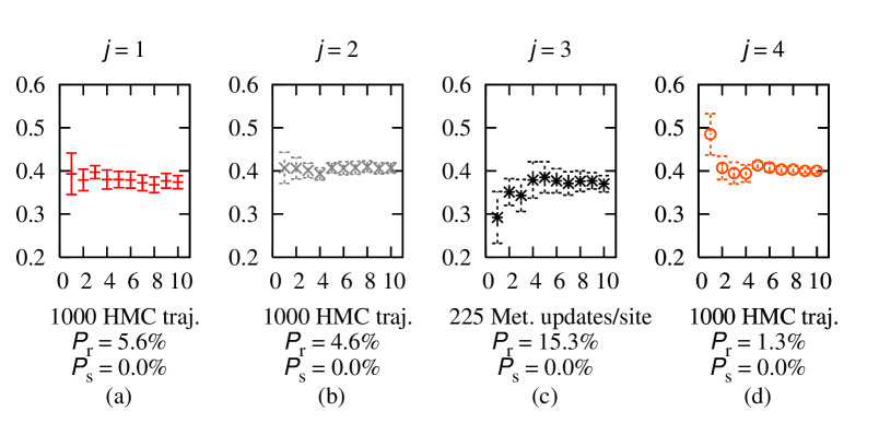
All four calculations are in agreement with an average value . In all cases the estimated errors are relatively small. In order of increasing error, the error bars for is smallest, then , , and . This is the same ordering we get by sorting rejection probability from lowest to highest. The singular matrix probability is zero in all cases.
Results for are shown in Fig. 4.

This time all four calculations are in agreement with . In all cases the estimated errors are still rather small, but upon closer inspection there are some early signs of trouble for and . For the rejection probability is quite large. This suggests difficulties in sampling the space of discrete auxiliary-field configurations. For the singular matrix probability is . This is approaching the level where the contribution due to singular matrices may be detectable above the background of stochastic error.
Results for are shown in Fig. 5.
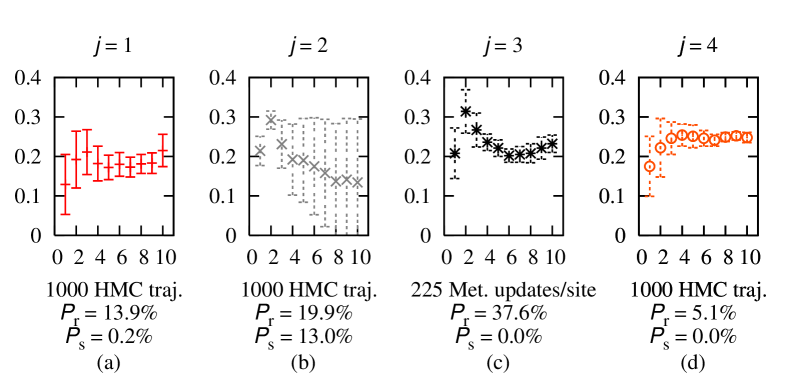
The simulation for has failed due to the high singular matrix probability. The calculations for are consistent with a value of . However the rejection probability for is very high. This could explain the gradual downward and then upward drift in the data, a sign that the Monte Carlo simulation has not fully equilibrated due to a long autocorrelation time. The same is true to a lesser extent for . For we also see that is small but nonzero. This suggests that problems with singular matrices may appear for somewhat larger and .
From this analysis we rate the performance for superior to the other three methods. This is not entirely unexpected. The use of a bounded auxiliary field should reduce the likelihood of exceptional configurations producing singular matrices. The use of a continuous auxiliary field makes it possible to use hybrid Monte Carlo which is better at reducing rejection probability than local Metropolis updates. For fixed trajectory length , the rejection probability for hybrid Monte Carlo scales quadratically with step size, . This is in contrast with the Metropolis algorithm, where the rejection probability scales linearly with the fraction of lattice sites updated in each sweep. This contributes to a much slower performance of the Metropolis algorithm at large and .
VI Main results
We use the bounded continuous auxiliary-field formulation for the lattice results presented in this section. We consider the unpolarized ten-particle and the fourteen-particle systems. For the calculation of we use the lattice dimensions shown in Table 3. For we use the lattice dimensions in Table 4.
|
|
|
|
|
|
We use trajectory parameters , and singular matrix parameter . The rejection probability reaches a maximum of and the singular matrix probability reaches a maximum of for the largest lattice volume, and . For most of the lattice simulations the values for and are much smaller. The simulations are run with a minimum of processors each running a minimum of hybrid Monte Carlo trajectories.
From Eq. (53) we expect
| (76) |
at large . To extract we perform a least squares fit of to the functional form,
| (77) |
For asymptotically large , we can identify with the energy separation between the ground state and the first excited state, possibly with degenerate partners. For large the lowest excitation is expected to be a two phonon state with zero total momentum. For large the excitation energy for this state is small compared with and therefore .
Our observable is proportional to the expectation value of the energy. When the energy difference is very small compared to the contribution proportional to is difficult to resolve against the background of stochastic noise. We note the factor
| (78) |
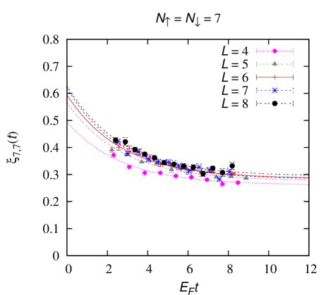
multiplying in Eq. (76). If the objective were to measure accurately for very low excitations, then it would be more effective to compute the Euclidean time projection of some other observable such as the difermion spatial correlation function
| (79) |
This technique was used to identify the lowest energy excitations for several unpolarized lattice systems at unitarity Lee (2007).
In the analysis here we focus only on measuring the ground state energy accurately and ignore the numerically small contributions hidden in the asymptotic tail of . We determine from least squares fitting over the range to . The values and we determine from least squares fitting should be interpreted as a spectral average,
| (80) |
Since has a well-defined continuum limit for fixed , each of the dimensionless parameters also has a well-defined continuum limit. Up to uncertainties the size of least squares fitting errors, is independent of the initial state overlap amplitudes . However and both depend on . Table 5 shows the three-parameter fit results for and Table 6 shows the three-parameter fit results for .
/d.f.
/d.f.
The average chi-square per degree of freedom for the fits is about . The error estimates for the fit parameters are calculated by explicit simulation. We introduce Gaussian-random noise scaled by the error bars of each data point for . The fit is repeated many times with the random noise included to estimate the one standard-deviation spread in the fit parameters.
The error in would be considerably smaller if the fit needed only two parameters rather than three parameters. This can be arranged if we neglect the -dependence of and fix according to the average values for as quoted in Tables 5 and 6. Since has a well-defined continuum limit, the -dependence of should in fact be small. For the average value is , and for the average value is . Using these values we refit with the two parameters . Table 7 shows the two-parameter fit results for and Table 8 shows the two-parameter fit results for .
/d.f.
/d.f.
The average chi-square per degree of freedom is again about . The lattice data for together with the two-parameter fit functions are shown Fig. 6.
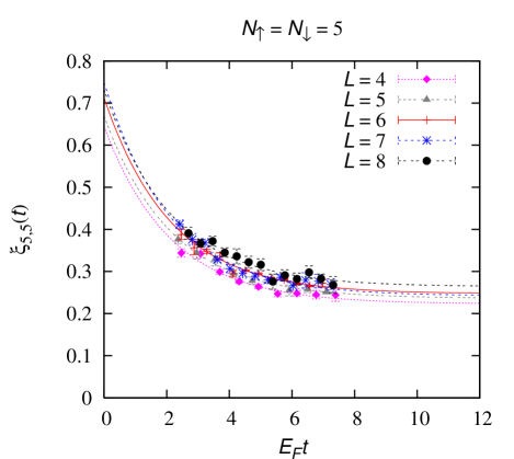
Fig. 7 shows the lattice data for with two-parameter fit functions.
The lattice results show that and are both approximately universal functions of independent of . This was expected from the scale invariance of the unitarity limit.
Using the results for and for we can extrapolate to the continuum limit . We expect some residual dependence on proportional to arising from effects such as the effective range correction, broken Galilean invariance, and possibly other lattice cutoff effects. From the three-parameter fit results in Tables 5 and 6, the linear extrapolation in gives the continuum limit values
| (81) |
| (82) |
If we extrapolate the two-parameter fit results in Tables 7 and 8 we get
| (83) |
| (84) |
Results from the two-parameter fits for and at finite and the corresponding continuum limit extrapolations are shown in Fig. 8.

We note that the continuum limit fit for could also be performed with defined in the continuum limit for the same cubic box size. This procedure is not recommended since it introduces a larger dependence and degrades the quality of the linear fit. However the fit can be done and the extrapolated values for and are each about higher than the values reported in Eq. (83) and (84) with somewhat larger error bars.
VII Discussion
In Lee (2006a) the values
| (85) |
| (86) |
were found based on an average of lattice results for . The results here for and with are consistent with these values. The continuum limit extrapolation was not possible in Lee (2006a) due to problems with increasing singular matrix probability . That calculation used the auxiliary field formulation which had the largest of the four methods considered here. The bounded continuous auxiliary-field method appears to solve this problem for the lattice systems considered here. The values for and from small lattices are each shifted upwards by when extrapolated to the continuum limit.
In the calculations presented here we have only considered systems with and particles and have not attempted to determine the thermodynamical limit . It is therefore interesting to compare with results obtained using other methods that have computed ground state energies for both small and large values of . Each of these other methods contain some unknown systematic errors, and so a benchmark comparison with continuum extrapolated Monte Carlo lattice results for and provides an estimate of the systematic error.
There is a discrepancy of about in the reported values for and between continuum extrapolated lattice results and fixed-node Green’s function Monte Carlo results on a periodic cube. The fixed-node Green’s function Monte Carlo simulations find for Carlson et al. (2003) and for larger Astrakharchik et al. (2004); Carlson and Reddy (2005). This discrepancy suggests that the upper bound on the ground state energy using fixed-node Green’s function Monte Carlo might be lowered further by a more optimal fermionic nodal surface.
A recent Hamiltonian lattice study computed for the range to on cubic lattices up to Lee (2008). This calculation used a method called the symmetric heavy-light ansatz in the lowest filling approximation. In Fig. 9 we compare Monte Carlo lattice results presented here and symmetric heavy-light ansatz results for and .
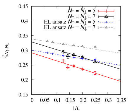
The continuum limit extrapolations of the symmetric heavy-light results give
| (87) |
| (88) |
These results are within of the values found in Eq. (83) and (84). This level of accuracy is consistent with the size of errors found in Lee (2008) for four-body and six-body systems of the 1D, 2D, 3D attractive Hubbard models at arbitrary coupling.
The different slopes for the Hamiltonian lattice and Euclidean lattice extrapolations in Fig. 9 are consistent with the fact that the effective range for the Hamiltonian lattice interaction is a smaller negative fraction of the lattice spacing than for the Euclidean lattice transfer matrix. However there are other effects such as broken Galilean invariance on the lattice which produce a similar dependence Lee and Thomson (2007). An accurate calculation of the effective range correction with controlled systematic errors requires either an effective range larger than the lattice spacing or an analysis of the effect of changing the effective range parameter relative to the lattice spacing. The effective range correction has recently been computed on the lattice with realistic dilute neutron matter at next-to-leading order in chiral effective field theory Borasoy et al. (2007b); Borasoy et al. (2008).
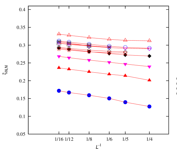
Results from the symmetric heavy-light ansatz for general are shown in Fig. 10 Lee (2008). We note that the value for reaches a maximum at . This can be explained by the closed shell at in the free fermion ground state and the absence of shell effects in the interacting system. The numerical agreement for the benchmark comparisons at and provides some confidence in the symmetric heavy-light ansatz value of for the unitarity limit in the continuum and thermodynamic limits Lee (2008).
The bounded continuous auxiliary-field method succeeds in reducing the singular matrix probability by minimizing large fluctuations in the auxiliary-field transfer matrix elements. Very roughly this corresponds with reducing the size of
| (89) |
given the constraints
| (90) |
| (91) |
| (92) |
For lattice systems larger than the ones considered here the problem with singular matrices will reappear. For very large systems there may be no choice but to use the stabilization methods developed in Sugiyama and Koonin (1986); Sorella et al. (1989); White et al. (1989) to reduce round-off error and confront the problems of large fluctuations and quasi-non-ergodic behavior using brute-force large-scale simulations. However for moderately larger systems it may be possible to gain further advantage using a function with a steep slope at and relatively flat away from zero. The most extreme case would be to use an odd periodic step function. But this is equivalent to the discrete auxiliary-field formulation with the problems discussed concerning large rejection probabilities. However with a smooth approximation to an odd periodic step function, it may be possible to reduce the singular matrix probability while at the same time compensate for the increase in rejection probability with a smaller hybrid Monte Carlo step size,
VIII Summary
We have presented new Euclidean lattice methods which remove some computational barriers encountered in previous lattice calculations of the ground state energy in the unitarity limit. We compared the performance of four different auxiliary-field methods that produce exactly the same lattice transfer matrix. By far the best performance was obtained using a bounded continuous auxiliary field with hybrid Monte Carlo updating. With this method we calculated results for and fermions at lattice volumes and extrapolated to the continuum limit. For fermions in a periodic cube, we found the ground state energy to be times the ground state energy for non-interacting fermions. For fermions the ratio is . These values may be useful as benchmarks for calculations of the unitarity limit ground state using other methods.
Acknowledgements
The author is grateful for discussions with Cliff Chafin, Gautam Rupak, and Thomas Schäfer. This work is supported in part by DOE grant DE-FG02-03ER41260.
References
- Eagles (1969) D. M. Eagles, Phys. Rev. 186, 456 (1969).
- Leggett (1980) A. J. Leggett, in Modern Trends in the Theory of Condensed Matter. Proceedings of the XVIth Karpacz Winter School of Theoretical Physics, Karpacz, Poland, 1980 (Springer-Verlag, Berlin, 1980), p. 13.
- Nozieres and Schmitt-Rink (1985) P. Nozieres and S. Schmitt-Rink, J. Low Temp. Phys. 59, 195 (1985).
- Pethick and Ravenhall (1995) C. J. Pethick and D. G. Ravenhall, Ann. Rev. Nucl. Part. Sci. 45, 429 (1995).
- Lattimer and Prakash (2004) J. M. Lattimer and M. Prakash, Science 304, 536 (2004), eprint astro-ph/0405262.
- O’Hara et al. (2002) K. M. O’Hara, S. L. Hemmer, M. E. Gehm, S. R. Granade, and J. E. Thomas, Science 298, 2179 (2002).
- Gupta et al. (2003) S. Gupta, Z. Hadzibabic, M. W. Zwierlein, C. A. Stan, K. Dieckmann, C. H. Schunck, E. G. M. van Kempen, B. J. Verhaar, and W. Ketterle, Science 300, 1723 (2003).
- Regal and Jin (2003) C. A. Regal and D. S. Jin, Phys. Rev. Lett. 90, 230404 (2003).
- Bourdel et al. (2003) T. Bourdel, J. Cubizolles, L. Khaykovich, K. M. F. Magalhaes, S. J. J. M. F. Kokkelmans, G. V. Shlyapnikov, and C. Salomon, Phys. Rev. Lett. 91, 020402 (2003).
- Gehm et al. (2003) M. E. Gehm, S. L. Hemmer, S. R. Granade, K. M. O’Hara, and J. E. Thomas, Phys. Rev. A68, 011401(R) (2003).
- Bartenstein et al. (2004) M. Bartenstein, A. Altmeyer, S. Riedl, S. Jochim, C. Chin, J. Hecker Denschlag, and R. Grimm, Phys. Rev. Lett. 92, 120401 (2004).
- Kinast et al. (2005) J. Kinast, A. Turlapov, J. E. Thomas, Q. Chen, J. Stajic, and K. Levin, Science 307, 1296 (2005), eprint cond-mat/0502087.
- Stewart et al. (2006) J. T. Stewart, J. P. Gaebler, C. A. Regal, and D. S. Jin, Phys. Rev. Lett. 97, 220406 (2006), eprint cond-mat/0607776.
- Engelbrecht et al. (1997) J. R. Engelbrecht, M. Randeria, and C. S. de Melo, Phys. Rev. B55, 15153 (1997).
- Baker (1999) G. A. Baker, Phys. Rev. C60, 054311 (1999).
- Heiselberg (2001) H. Heiselberg, Phys. Rev. A63, 043606 (2001), eprint cond-mat/0002056.
- Perali et al. (2004) A. Perali, P. Pieri, and G. C. Strinati, Phys. Rev. Lett. 93, 100404 (2004).
- Schäfer et al. (2005) T. Schäfer, C.-W. Kao, and S. R. Cotanch, Nucl. Phys. A762, 82 (2005), eprint nucl-th/0504088.
- Papenbrock (2005) T. Papenbrock, Phys. Rev. A72, 041603 (2005), eprint cond-mat/0507183.
- Nishida and Son (2006) Y. Nishida and D. T. Son, Phys. Rev. Lett. 97, 050403 (2006), eprint cond-mat/0604500.
- Nishida and Son (2007) Y. Nishida and D. T. Son, Phys. Rev. A75, 063617 (2007), eprint cond-mat/0607835.
- Chen (2007) J. Chen, Chinese Phys. Lett 24, 1825 (2007), eprint nucl-th/0602065.
- Krippa (2007) B. Krippa (2007), eprint arXiv:0704.3984 [cond-mat.supr-con].
- Arnold et al. (2007) P. Arnold, J. E. Drut, and D. T. Son, Phys. Rev. A75, 043605 (2007), eprint cond-mat/0608477.
- Nikolic and Sachdev (2007) P. Nikolic and S. Sachdev, Phys. Rev. A75, 033608 (2007), eprint cond-mat/0609106.
- Veillette et al. (2007) M. Y. Veillette, D. E. Sheehy, and L. Radzihovsky, Phys. Rev. A75, 043614 (2007), eprint cond-mat/0610798.
- Carlson et al. (2003) J. Carlson, S. Y. Chang, V. R. Pandharipande, and K. Schmidt, Phys. Rev. Lett. 91, 50401 (2003), eprint physics/0303094.
- Astrakharchik et al. (2004) G. E. Astrakharchik, J. Boronat, J. Casulleras, and S. Giorgini, Phys. Rev. Lett. 93, 200404 (2004), eprint cond-mat/0406113.
- Carlson and Reddy (2005) J. Carlson and S. Reddy, Phys. Rev. Lett. 95, 060401 (2005), eprint cond-mat/0503256.
- Akkineni et al. (2006) V. K. Akkineni, D. M. Ceperley, and N. Trivedi (2006), eprint cond-mat/0608154.
- Juillet (2007) O. Juillet, New Journal of Physics 9, 163 (2007), eprint cond-mat/0609063.
- Bulgac et al. (2006) A. Bulgac, J. E. Drut, and P. Magierski, Phys. Rev. Lett. 96, 090404 (2006), eprint cond-mat/0505374.
- Bulgac et al. (2008) A. Bulgac, J. E. Drut, P. Magierski, and G. Wlazlowski (2008), eprint arXiv:0801.1504 [cond-mat.stat-mech].
- Burovski et al. (2006a) E. Burovski, N. Prokofev, B. Svistunov, and M. Troyer, Phys. Rev. Lett. 96, 160402 (2006a), eprint cond-mat/0602224.
- Burovski et al. (2006b) E. Burovski, N. Prokofev, B. Svistunov, and M. Troyer, New J. Phys. 8, 153 (2006b), eprint cond-mat/0605350.
- Lee and Schäfer (2006a) D. Lee and T. Schäfer, Phys. Rev. C73, 015201 (2006a), eprint nucl-th/0509017.
- Lee and Schäfer (2006b) D. Lee and T. Schäfer, Phys. Rev. C73, 015202 (2006b), eprint nucl-th/0509018.
- Abe and Seki (2007a) T. Abe and R. Seki (2007a), eprint arXiv:0708.2523 [nucl-th].
- Abe and Seki (2007b) T. Abe and R. Seki (2007b), eprint arXiv:0708.2524 [nucl-th].
- Lee (2006a) D. Lee, Phys. Rev. B73, 115112 (2006a), eprint cond-mat/0511332.
- Lee (2008) D. Lee, Eur. Phys. J. A35, 171 (2008), eprint arXiv:0704.3439 [cond-mat.supr-con].
- Lee (2007) D. Lee, Phys. Rev. B75, 134502 (2007), eprint cond-mat/0606706.
- Duane et al. (1987) S. Duane, A. D. Kennedy, B. J. Pendleton, and D. Roweth, Phys. Lett. B195, 216 (1987).
- Lüscher (1986) M. Lüscher, Commun. Math. Phys. 105, 153 (1986).
- Beane et al. (2004) S. R. Beane, P. F. Bedaque, A. Parreno, and M. J. Savage, Phys. Lett. B585, 106 (2004), eprint hep-lat/0312004.
- Seki and van Kolck (2006) R. Seki and U. van Kolck, Phys. Rev. C73, 044006 (2006), eprint nucl-th/0509094.
- Borasoy et al. (2007a) B. Borasoy, E. Epelbaum, H. Krebs, D. Lee, and U.-G. Meißner, Eur. Phys. J. A31, 105 (2007a), eprint nucl-th/0611087.
- Lee and Schäfer (2005) D. Lee and T. Schäfer, Phys. Rev. C72, 024006 (2005), eprint nucl-th/0412002.
- Creutz (1988) M. Creutz, Phys. Rev. D38, 1228 (1988).
- Creutz (2000) M. Creutz, Found. Phys. 30, 487 (2000), eprint hep-lat/9905024.
- Stratonovich (1958) R. L. Stratonovich, Soviet Phys. Doklady 2, 416 (1958).
- Hubbard (1959) J. Hubbard, Phys. Rev. Lett. 3, 77 (1959).
- Hirsch (1983) J. E. Hirsch, Phys. Rev. B28, 4059 (1983).
- Lee (2006b) D. Lee, Phys. Rev. A73, 063204 (2006b), eprint physics/0512085.
- Sugiyama and Koonin (1986) G. Sugiyama and S. E. Koonin, Ann. Phys. 168, 1 (1986).
- Sorella et al. (1989) S. Sorella, S. Baroni, R. Car, and M. Parrinello, Europhys. Lett. 8, 663 (1989).
- White et al. (1989) S. R. White, D. J. Scalapino, R. L. Sugar, E. Y. Loh, J. E. Gubernatis, and R. T. Scalettar, Phys. Rev. B 40, 506 (1989).
- Lee and Thomson (2007) D. Lee and R. Thomson, Phys. Rev. C75, 064003 (2007), eprint nucl-th/0701048.
- Borasoy et al. (2007b) B. Borasoy, E. Epelbaum, H. Krebs, D. Lee, and U.-G. Meißner, Eur. Phys. J. A34, 185 (2007b), eprint arXiv:0708.1780 [nucl-th].
- Borasoy et al. (2008) B. Borasoy, E. Epelbaum, H. Krebs, D. Lee, and U.-G. Meissner, Eur. Phys. J. A35, 357 (2008), eprint arXiv:0712.2993 [nucl-th].