Parameter Collapse due to the Zeros in the Inverse Condition

R.Β Spjut spjut@math.ucsb.edu [ Department of Mathematics, University of California, Santa Barbara, CA 93106
(7 Feb 2008)
Abstract

Helton, Lasserre, and Putinar (2008, Ann. Probability; arXiv:math/0702314) expose the relationship between three properties of a measure: the conditional triangularity property of the associated orthogonal polynomials, the zeros in the inverse condition of the truncated moment matrix, and conditional independence. The purpose of this article is to provide examples of parameter collapse to product structure given that the zeros in the inverse condition holds up to some degree d𝑑d. Specifically, start with a parameterized family of probability density functions; require that the zeros in the inverse condition up to degree d𝑑d holds; and validate that imposing this restriction on the parameterized family results in a measure with product structure, or at least that conditional independence holds. Algorithms related to parameter collapse are supplied, including the computation of the zeros in the inverse condition up to degree d𝑑d.

keywords:
moment matrix , truncated moment matrix , independence , conditional independence , parameterized distributions
MSC:
47N30 , 47A57 , 15-04 , 44A60

url]http://math.ucsb.edu/∼similar-to\simspjut/ ††thanks: Work supported by the UCSB and the NSF. Special thanks to Mihai Putinar.

1 Introduction

Generalization of independence certificates for multivariate probability distributions is exciting. For instance, techniques such as those found in [2] could be generalized to non-normal variables. As a specific example, near the variable bounds of instrument operation error distributions are known to be non-Gaussian. In short, if a data set is fitted by a particular family of multivariate distributions, the algorithms supplied in this article provide a statistician with the knowledge of precisely how many moments must be calculated to ensure variables are independent, or at least conditionally independent.

This is perhaps the most interesting aspect, that parameter collapse to product structure can require computation of moment matrices of order greater than 2. To exhibit independence of variables for multivariate Gaussian distributions one much check the truncated moments only up to order 2, but proving independence of variables for some distributions requires higher moments. When a parameterized family of distributions exhibits parameter collapse, the minimum order of the zeros in the inverse condition required for the measure to exhibit product structure is called the parameter collapse order of the parameterized measure [1, Β§6 Definition 3].

Finally, the computations of moments of polynomials by hand is tedious, at best. Maple routines are provided in the appendix to automate computations. Furthermore, a program is available upon request that computes the parameter collapse order of a particular family of multivariate measures. Assistance for translation to other computer algebra systems or languages is offered and code is immediately available in Maple, Mathematica, Matlab, C, and Java. In particular, it may prove beneficial to integrate these routines with existing, high-powered software [3].

The following examples are meant to provide elementary exposition of the analysis discussed above.

2 Examples

2.1 Preliminary example

Consider the following parameterized multivariate distribution with product structure. Let X1,X2,X3subscript𝑋1subscript𝑋2subscript𝑋3X_{1},X_{2},X_{3} be independent Poisson processes on ℝ+=(0,∞)subscriptℝ0\mathbb{R}_{+}=(0,\infty) with probability density

pΞ»,k​(x)={Ξ»k​xkβˆ’1​eβˆ’Ξ»β€‹xΓ​(k)xβ‰₯00x<0;Γ​(k)=∫0∞tkβˆ’1​eβˆ’t​𝑑t.formulae-sequencesubscriptπ‘πœ†π‘˜π‘₯casessuperscriptπœ†π‘˜superscriptπ‘₯π‘˜1superscriptπ‘’πœ†π‘₯Ξ“π‘˜π‘₯00π‘₯0Ξ“π‘˜superscriptsubscript0superscriptπ‘‘π‘˜1superscript𝑒𝑑differential-d𝑑p_{\lambda,k}(x)=\left\{\begin{array}[]{cc}\frac{\lambda^{k}x^{k-1}e^{-\lambda x}}{\Gamma(k)}&x\geq 0\\ 0&x<0\end{array}\right.;\Gamma(k)=\int_{0}^{\infty}t^{k-1}e^{-t}dt.

Let λ​τ=xπœ†πœπ‘₯\lambda\tau=x and for simplicity, Ξ»=1πœ†1\lambda=1, so that the joint distribution is

pk1,k2,k3​(x1,x2,x3)=eβˆ’x1​x1k1βˆ’1Γ​(k1)​eβˆ’x2​x2k2βˆ’1Γ​(k2)​eβˆ’x3​x3k3βˆ’1Γ​(k3),subscript𝑝subscriptπ‘˜1subscriptπ‘˜2subscriptπ‘˜3subscriptπ‘₯1subscriptπ‘₯2subscriptπ‘₯3superscript𝑒subscriptπ‘₯1superscriptsubscriptπ‘₯1subscriptπ‘˜11Ξ“subscriptπ‘˜1superscript𝑒subscriptπ‘₯2superscriptsubscriptπ‘₯2subscriptπ‘˜21Ξ“subscriptπ‘˜2superscript𝑒subscriptπ‘₯3superscriptsubscriptπ‘₯3subscriptπ‘˜31Ξ“subscriptπ‘˜3p_{k_{1},k_{2},k_{3}}(x_{1},x_{2},x_{3})=\frac{e^{-x_{1}}x_{1}^{k_{1}-1}}{\Gamma(k_{1})}\frac{e^{-x_{2}}x_{2}^{k_{2}-1}}{\Gamma(k_{2})}\frac{e^{-x_{3}}x_{3}^{k_{3}-1}}{\Gamma(k_{3})},

a measure with product structure. To compute moments, we are led to the gamma function

E​(x1p​x2q)𝐸superscriptsubscriptπ‘₯1𝑝superscriptsubscriptπ‘₯2π‘ž\displaystyle E(x_{1}^{p}x_{2}^{q}) =\displaystyle= ∫0∞∫0∞x1p​x2q​eβˆ’x1​x1k1βˆ’1Γ​(k1)​eβˆ’x2​x2k2βˆ’1Γ​(k2)​𝑑x1​𝑑x2superscriptsubscript0superscriptsubscript0superscriptsubscriptπ‘₯1𝑝superscriptsubscriptπ‘₯2π‘žsuperscript𝑒subscriptπ‘₯1superscriptsubscriptπ‘₯1subscriptπ‘˜11Ξ“subscriptπ‘˜1superscript𝑒subscriptπ‘₯2superscriptsubscriptπ‘₯2subscriptπ‘˜21Ξ“subscriptπ‘˜2differential-dsubscriptπ‘₯1differential-dsubscriptπ‘₯2\displaystyle\int_{0}^{\infty}\int_{0}^{\infty}x_{1}^{p}x_{2}^{q}\frac{e^{-x_{1}}x_{1}^{k_{1}-1}}{\Gamma(k_{1})}\frac{e^{-x_{2}}x_{2}^{k_{2}-1}}{\Gamma(k_{2})}dx_{1}dx_{2}
=\displaystyle= ∫0∞eβˆ’x1​x1p+k1βˆ’1Γ​(k1)​𝑑x1β€‹βˆ«0∞eβˆ’x2​x2q+k2βˆ’1Γ​(k2)​𝑑x2superscriptsubscript0superscript𝑒subscriptπ‘₯1superscriptsubscriptπ‘₯1𝑝subscriptπ‘˜11Ξ“subscriptπ‘˜1differential-dsubscriptπ‘₯1superscriptsubscript0superscript𝑒subscriptπ‘₯2superscriptsubscriptπ‘₯2π‘žsubscriptπ‘˜21Ξ“subscriptπ‘˜2differential-dsubscriptπ‘₯2\displaystyle\int_{0}^{\infty}\frac{e^{-x_{1}}x_{1}^{p+k_{1}-1}}{\Gamma(k_{1})}dx_{1}\int_{0}^{\infty}\frac{e^{-x_{2}}x_{2}^{q+k_{2}-1}}{\Gamma(k_{2})}dx_{2}
=\displaystyle= Γ​(p+k1)​Γ​(q+k2)Γ​(k1)​Γ​(k2)=p!​q!.Γ𝑝subscriptπ‘˜1Ξ“π‘žsubscriptπ‘˜2Ξ“subscriptπ‘˜1Ξ“subscriptπ‘˜2π‘π‘ž\displaystyle\frac{\Gamma(p+k_{1})\Gamma(q+k_{2})}{\Gamma(k_{1})\Gamma(k_{2})}=p!q!.

For X1subscript𝑋1X_{1} and X2subscript𝑋2X_{2}, M1subscript𝑀1M_{1} and M1βˆ’1superscriptsubscript𝑀11M_{1}^{-1} are:

1x1x21111x1121x2112M1βˆ’1=[3βˆ’1βˆ’1βˆ’110βˆ’101].missing-subexpression1subscriptπ‘₯1subscriptπ‘₯2missing-subexpressionmissing-subexpressionmissing-subexpressionmissing-subexpression1111subscriptπ‘₯1121subscriptπ‘₯2112missing-subexpressionsuperscriptsubscript𝑀11delimited-[]311missing-subexpressionmissing-subexpressionmissing-subexpression110missing-subexpressionmissing-subexpressionmissing-subexpression101\begin{array}[]{ccc}\begin{array}[]{c|ccc}&1&x_{1}&x_{2}\\ \hline\cr 1&1&1&1\\ x_{1}&1&2&1\\ x_{2}&1&1&2\end{array}&&M_{1}^{-1}=\left[\begin{array}[]{ccc}3&-1&-1\\ \vskip 6.0pt plus 2.0pt minus 2.0pt\cr-1&1&0\\ \vskip 6.0pt plus 2.0pt minus 2.0pt\cr-1&0&1\end{array}\right]\end{array}.

From [1, Theorem 5], the zeros in the inverse property is equivalent to the orthogonal polynomials satisfying the conditional triangularity. For X1subscript𝑋1X_{1} and X2subscript𝑋2X_{2}, M2subscript𝑀2M_{2} and M2βˆ’1superscriptsubscript𝑀21M_{2}^{-1} are:

1x1x2x12x1​x2x221111212x1121622x2112226x122622464x1​x2122646x222264624M2βˆ’1=[6βˆ’4βˆ’41/211/2βˆ’461βˆ’1βˆ’10βˆ’4160βˆ’1βˆ’11/2βˆ’101/4001βˆ’1βˆ’10101/20βˆ’1001/4].missing-subexpression1subscriptπ‘₯1subscriptπ‘₯2superscriptsubscriptπ‘₯12subscriptπ‘₯1subscriptπ‘₯2superscriptsubscriptπ‘₯22missing-subexpressionmissing-subexpressionmissing-subexpressionmissing-subexpressionmissing-subexpressionmissing-subexpressionmissing-subexpression1111212subscriptπ‘₯1121622subscriptπ‘₯2112226superscriptsubscriptπ‘₯122622464subscriptπ‘₯1subscriptπ‘₯2122646superscriptsubscriptπ‘₯222264624missing-subexpressionsuperscriptsubscript𝑀21delimited-[]64412112missing-subexpressionmissing-subexpressionmissing-subexpression461110missing-subexpressionmissing-subexpressionmissing-subexpression416011missing-subexpressionmissing-subexpressionmissing-subexpression12101400missing-subexpressionmissing-subexpressionmissing-subexpression111010missing-subexpressionmissing-subexpressionmissing-subexpression12010014\begin{array}[]{ccc}\begin{array}[]{c|cccccc}&1&x_{1}&x_{2}&x_{1}^{2}&x_{1}x_{2}&x_{2}^{2}\\ \hline\cr 1&1&1&1&2&1&2\\ x_{1}&1&2&1&6&2&2\\ x_{2}&1&1&2&2&2&6\\ x_{1}^{2}&2&6&2&24&6&4\\ x_{1}x_{2}&1&2&2&6&4&6\\ x_{2}^{2}&2&2&6&4&6&24\end{array}&&M_{2}^{-1}=\left[\begin{array}[]{cccccc}6&-4&-4&1/2&1&1/2\\ \vskip 6.0pt plus 2.0pt minus 2.0pt\cr-4&6&1&-1&-1&0\\ \vskip 6.0pt plus 2.0pt minus 2.0pt\cr-4&1&6&0&-1&-1\\ \vskip 6.0pt plus 2.0pt minus 2.0pt\cr 1/2&-1&0&1/4&0&0\\ \vskip 6.0pt plus 2.0pt minus 2.0pt\cr 1&-1&-1&0&1&0\\ \vskip 6.0pt plus 2.0pt minus 2.0pt\cr 1/2&0&-1&0&0&1/4\end{array}\right].\end{array}

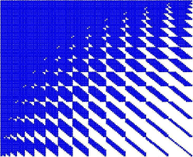
Compare M2βˆ’1superscriptsubscript𝑀21M_{2}^{-1} with Figure 1.

Refer to caption
Refer to caption
Figure 1: Zeros In the Inverse Condition for d=2 and d=14, respectively. The blue dots indicate non-zero entries.

2.2 First example of parameter collapse to product structure

Let β„“β„“\ell be a nonnegative integer. Given the bivariate distribution defined on the positive quadrant:

pℓ​(x,y)=1C​(β„“)​eβˆ’(x+y)​(x+y)β„“,subscript𝑝ℓπ‘₯𝑦1𝐢ℓsuperscript𝑒π‘₯𝑦superscriptπ‘₯𝑦ℓ\displaystyle p_{\ell}(x,y)=\frac{1}{C(\ell)}e^{-(x+y)}(x+y)^{\ell}, (1)

where C​(β„“)=βˆ‘j=0β„“β„“!​(β„“βˆ’j+1)​(j+1)𝐢ℓsuperscriptsubscript𝑗0ℓℓℓ𝑗1𝑗1C(\ell)=\sum_{j=0}^{\ell}\ell!(\ell-j+1)(j+1).

Calculate M1βˆ’1superscriptsubscript𝑀11M_{1}^{-1} and set the (3,2)32(3,2) which is the (2,3)23(2,3) entry to zero. Skipping messy details, this reduces to:

0=v​(β„“)0𝑣ℓ\displaystyle 0=v(\ell) ≑\displaystyle\equiv (∫0∞∫0∞pℓ​(x,y)​𝑑x​𝑑y)​(∫0∞∫0∞x​y​pℓ​(x,y)​𝑑x​𝑑y)superscriptsubscript0superscriptsubscript0subscript𝑝ℓπ‘₯𝑦differential-dπ‘₯differential-d𝑦superscriptsubscript0superscriptsubscript0π‘₯𝑦subscript𝑝ℓπ‘₯𝑦differential-dπ‘₯differential-d𝑦\displaystyle\left(\int_{0}^{\infty}\int_{0}^{\infty}p_{\ell}(x,y)dxdy\right)\left(\int_{0}^{\infty}\int_{0}^{\infty}xyp_{\ell}(x,y)dxdy\right)
βˆ’(∫0∞∫0∞x​pℓ​(x,y)​𝑑x​𝑑y)2superscriptsuperscriptsubscript0superscriptsubscript0π‘₯subscript𝑝ℓπ‘₯𝑦differential-dπ‘₯differential-d𝑦2\displaystyle-\left(\int_{0}^{\infty}\int_{0}^{\infty}xp_{\ell}(x,y)dxdy\right)^{2}

It can be shown that v​(β„“)<0𝑣ℓ0v(\ell)<0 for β„“β‰₯1β„“1\ell\geq 1. Therefore, β„“=0β„“0\ell=0 is the only solution which satisfies the zeros in the inverse property for the first truncated moment matrix, and p0​(x,y)=eβˆ’x​eβˆ’ysubscript𝑝0π‘₯𝑦superscript𝑒π‘₯superscript𝑒𝑦p_{0}(x,y)=e^{-x}e^{-y} has the product structure indicating independence. The parameter collapse order of pℓ​(x,y)subscript𝑝ℓπ‘₯𝑦p_{\ell}(x,y) is 1. Remark that there are a number of similar, parameterized, bivariate, exponential distributions that exhibit parameter collapse.

2.3 A bivariate exponential non-example

A multivariate Gamma distribution studied in [4, Chpt 41Β§3] is:

pΟƒ1,Οƒ2,ρ​(x,y)=1Οƒ1​σ2​(1βˆ’Ο)​eβˆ’11βˆ’Οβ€‹(x1Οƒ1+x2Οƒ2)​I0​(2​ρ1βˆ’Οβ€‹x1​x2Οƒ1​σ2),subscript𝑝subscript𝜎1subscript𝜎2𝜌π‘₯𝑦1subscript𝜎1subscript𝜎21𝜌superscript𝑒11𝜌subscriptπ‘₯1subscript𝜎1subscriptπ‘₯2subscript𝜎2subscript𝐼02𝜌1𝜌subscriptπ‘₯1subscriptπ‘₯2subscript𝜎1subscript𝜎2p_{\sigma_{1},\sigma_{2},\rho}(x,y)=\frac{1}{\sigma_{1}\sigma_{2}(1-\rho)}e^{-\frac{1}{1-\rho}\left(\frac{x_{1}}{\sigma_{1}}+\frac{x_{2}}{\sigma_{2}}\right)}I_{0}\left(\frac{2\sqrt{\rho}}{1-\rho}\sqrt{\frac{x_{1}x_{2}}{\sigma_{1}\sigma_{2}}}\right),

where I0subscript𝐼0I_{0} is the modified Bessel function of first order (with v=2𝑣2v=2).

Solve the collapsing of parameters problems via the Maple code provided in the appendix and the following lines:

Β 

> assume(sigma1>0); assume(sigma2>0); assume(rho <1);
> additionally(rho >0);
> f:= (x,y) -> (1/(sigma1*sigma2*(1-rho)))*
     exp(-(1/(1-rho))*(x/sigma1+y/sigma2))*
     BesselJ(2,2*sqrt(rho*x*y/sigma1/sigma2)/(1-rho));
> equations := zerosInInverse(f,1);

Β 

A zero in the (3,2)32(3,2) entry of the first truncated moment matrix implies

βˆ’(1βˆ’Ο)2​(ρ2+2​ρ​(1βˆ’ln⁑(1+ρ))βˆ’2​ln⁑(1+ρ))=0.superscript1𝜌2superscript𝜌22𝜌11𝜌21𝜌0-(1-\rho)^{2}\left(\rho^{2}+2\rho\left(1-\ln(1+\rho)\right)-2\ln(1+\rho)\right)=0.

The left hand side is zero only if ρ=0𝜌0\rho=0, but then pΟƒ1,Οƒ2,0​(x,y)=0subscript𝑝subscript𝜎1subscript𝜎20π‘₯𝑦0p_{\sigma_{1},\sigma_{2},0}(x,y)=0 is not a pdf. Thus, pΟƒ1,Οƒ2,ρ​(x,y)subscript𝑝subscript𝜎1subscript𝜎2𝜌π‘₯𝑦p_{\sigma_{1},\sigma_{2},\rho}(x,y) never has product structure.

2.4 An example with compact support

Consider a probability density function found in [5, Β§15.4],

p​d​fR​(x,y)=Γ​((v+2)/2)(π​v)1/2​Γ​(v/2)​(1+vβˆ’1​[xy]​R​[xy]),𝑝𝑑subscript𝑓𝑅π‘₯𝑦Γ𝑣22superscriptπœ‹π‘£12Γ𝑣21superscript𝑣1delimited-[]π‘₯𝑦𝑅delimited-[]π‘₯𝑦pdf_{R}(x,y)=\frac{\Gamma((v+2)/2)}{(\pi v)^{1/2}\Gamma(v/2)}\left(1+v^{-1}\left[\begin{array}[]{cc}x&y\\ \end{array}\right]R\left[\begin{array}[]{c}x\\ y\\ \end{array}\right]\right),

where R∈SL(2,ℝR\in SL(2,\mathbb{R} and (x,y)∈B​(0,1)βŠ‚β„2π‘₯𝑦𝐡01superscriptℝ2(x,y)\in B(0,1)\subset\mathbb{R}^{2}. Ignore the normalizing constant, with a​dβˆ’b​c=1π‘Žπ‘‘π‘π‘1ad-bc=1,

p​d​fR​(x,y)=1+1v​(a​x2+c​x​y+b​x​y+d​y2).𝑝𝑑subscript𝑓𝑅π‘₯𝑦11π‘£π‘Žsuperscriptπ‘₯2𝑐π‘₯𝑦𝑏π‘₯𝑦𝑑superscript𝑦2pdf_{R}(x,y)=1+\frac{1}{v}\left(ax^{2}+cxy+bxy+dy^{2}\right).

The first order zeros in the inverse condition reduces to c+b=0𝑐𝑏0c+b=0, implying:

p​d​fR​(x,y)=1+1v​(a​x2+d​y2).𝑝𝑑subscript𝑓𝑅π‘₯𝑦11π‘£π‘Žsuperscriptπ‘₯2𝑑superscript𝑦2pdf_{R}(x,y)=1+\frac{1}{v}\left(ax^{2}+dy^{2}\right).

The second order zeros in its inverse condition is:

0=3​a2+36​a+22​d​a+48+3​d2+36​d.03superscriptπ‘Ž236π‘Ž22π‘‘π‘Ž483superscript𝑑236𝑑0=3a^{2}+36a+22da+48+3d^{2}+36d.

From which four cases arise, all of which do not allow for solutions when the third order zeros in the inverse condition is imposed. Therefore, parameter collapse does not occur until degree three.

2.5 Polynomial and discrete pdfs

The previous section provided an example of parameter collapse requiring degree greater than 2. The computations were easier, as the only product structures allowed were trivial ones. Consider measures on [0,1]Γ—[0,1]0101[0,1]\times[0,1] of the form

βˆ‘k=0d​e​gβˆ‘β„“=0kak,kβˆ’β„“β€‹xk​ykβˆ’β„“.superscriptsubscriptπ‘˜0𝑑𝑒𝑔subscriptsuperscriptπ‘˜β„“0subscriptπ‘Žπ‘˜π‘˜β„“superscriptπ‘₯π‘˜superscriptπ‘¦π‘˜β„“\sum_{k=0}^{deg}\sum^{k}_{\ell=0}a_{k,k-\ell}x^{k}y^{k-\ell}.

In this case, positivity is required on [0,1]Γ—[0,1]0101[0,1]\times[0,1]. By integrating, we see:

For simplicity, ignore the above normalization constraint which would yield:

1=∫01∫01βˆ‘k=0d​e​gβˆ‘β„“=0kak,kβˆ’β„“β€‹xk​ykβˆ’β„“=βˆ‘k=0d​e​gβˆ‘β„“=0kak,kβˆ’β„“(k+1)​(kβˆ’β„“+1)1superscriptsubscript01superscriptsubscript01superscriptsubscriptπ‘˜0𝑑𝑒𝑔subscriptsuperscriptπ‘˜β„“0subscriptπ‘Žπ‘˜π‘˜β„“superscriptπ‘₯π‘˜superscriptπ‘¦π‘˜β„“superscriptsubscriptπ‘˜0𝑑𝑒𝑔subscriptsuperscriptπ‘˜β„“0subscriptπ‘Žπ‘˜π‘˜β„“π‘˜1π‘˜β„“11=\int_{0}^{1}\int_{0}^{1}\sum_{k=0}^{deg}\sum^{k}_{\ell=0}a_{k,k-\ell}x^{k}y^{k-\ell}=\sum_{k=0}^{deg}\sum^{k}_{\ell=0}\frac{a_{k,k-\ell}}{(k+1)(k-\ell+1)}
β‡’a00=1βˆ’βˆ‘k=1d​e​gβˆ‘β„“=0kak,kβˆ’β„“(k+1)​(kβˆ’β„“+1).β‡’absentsubscriptπ‘Ž001superscriptsubscriptπ‘˜1𝑑𝑒𝑔subscriptsuperscriptπ‘˜β„“0subscriptπ‘Žπ‘˜π‘˜β„“π‘˜1π‘˜β„“1\Rightarrow a_{00}=1-\sum_{k=1}^{deg}\sum^{k}_{\ell=0}\frac{a_{k,k-\ell}}{(k+1)(k-\ell+1)}.

Consider the measure:

p​d​fa0,0,a1,0,a0,1,a1,1​(x,y)=a1,1​x​y+a1,0​x+a0,1​y+a0,0𝑝𝑑superscript𝑓subscriptπ‘Ž00subscriptπ‘Ž10subscriptπ‘Ž01subscriptπ‘Ž11π‘₯𝑦subscriptπ‘Ž11π‘₯𝑦subscriptπ‘Ž10π‘₯subscriptπ‘Ž01𝑦subscriptπ‘Ž00pdf^{a_{0,0},a_{1,0},a_{0,1},a_{1,1}}(x,y)=a_{1,1}xy+a_{1,0}x+a_{0,1}y+a_{0,0}

The first order zeros in the inverse condition requires a11​a00=a10​a01subscriptπ‘Ž11subscriptπ‘Ž00subscriptπ‘Ž10subscriptπ‘Ž01a_{11}a_{00}=a_{10}a_{01}, which then would imply:

p​d​fa0,0,a1,0,a0,1,a1,1​(x,y)=1a11​(a10+a11​y)​(a11​x+a01)𝑝𝑑superscript𝑓subscriptπ‘Ž00subscriptπ‘Ž10subscriptπ‘Ž01subscriptπ‘Ž11π‘₯𝑦1subscriptπ‘Ž11subscriptπ‘Ž10subscriptπ‘Ž11𝑦subscriptπ‘Ž11π‘₯subscriptπ‘Ž01pdf^{a_{0,0},a_{1,0},a_{0,1},a_{1,1}}(x,y)=\frac{1}{a_{11}}(a_{10}+a_{11}y)(a_{11}x+a_{01})

which is of product form. Parameter collapse occurs in the first order. Parameter collapse for the most general polynomial and discrete measures of higher order result in only conditional independence. One interesting question is, which parameterized higher order polynomials exhibit parameter collapse to full independence? Note that the answer may yield irreducibility criterion.

3 Conclusion

There are a wealth of examples of parameter collapse due to the zeros in the inverse condition. One task related to other areas of research is automation of product form recognition for functions. Another unanswered question related to [6] is, β€œWhich polynomials may represent pdfs?” An interesting problem whose solution requires analysis of integral equations is, β€œFor integer n, what is the general form of pdfs that exhibit parameter collapse order n?” The latter two questions depend heavily upon the domain of the pdf.

Appendix A Maple Code

Here is a maple procedure that calculates the truncated moment matrix of order d𝑑d for the bivariate pdf, g​(x,y)𝑔π‘₯𝑦g(x,y); computes the inverse; and creates a list of equations generated from the zeros in the inverse condition.


Β 

> restart: with(linalg):
> zerosInInverse := proc(g::operator,d::integer)
>
> # set up the structure of the truncated moment matrix
> L:=[]:
> for i from 0 to d do
>    for j from 0 to i do
>       L:=[op(L),[i-j,j]]:
>    end do;
> end do;
>
> #fill truncated moment matrix using appropriate domain for g(x,y)
> B := (i,j) -> int(int(x^i*y^j*g(x,y),x=0..infinity,y=0..infinity);
> A:=matrix(nops(L),nops(L)):
> for i from 1 to nops(L) do
>    for j from 1 to nops(L) do
>       A[i,j] := B(L[i][1]+L[j][1],L[i][2]+L[j][2]);
>    end do;
> end do;
> C:= inverse(A);
>
> #Generate set of equations from zeros in inverse condition
> S:={};
> for i from 1 to nops(L) do
>    for j from i to nops(L) do
>       if (max(L[i][1],L[j][1])+max(L[i][2],L[j][2]) > d)
>       then S:={op(S),C[i,j]=0}; end if;
>    end do;
> end do;
> S
> end proc:

Β 

Thus, for a particular pdf, as in example 1.


Β 

> assume(ell::nonnegint);
> p:= (x,y) -> exp(-(x+y))*(x+y)^ell/(ell+1)!;
> equations = zerosInInverse(p,1);

Β 

The next step would be to run the following command.

Β 

> solve(equations);

Β 

References

  • [1] J.W.Β Helton, J.B.Β Lasserre, M.Β Putinar. Measures with zeros in the inverse of their moment matrix arXiv:math/0702314 to appear in Ann. Probability
  • [2] O.Β Banerjee, L.Β Ghaoui, A.Β d’Aspremont, G. Natsoulis. Convex Optimization Techniques for Fitting Sparse Gaussian Graphical Models International Conference on Machine Learning 2006, 2006.
  • [3] D.Β Henrion, J-B.Β Lasserre, J.Β Lofberg. GloptiPoly 3: moments, optimization and semidefinite programming arXiv:0709.2559
  • [4] S.Β Kotz, N.L.Β Johnson. Distributions in Statistics: Continuous Multivariate Distributions Vol II, John Wiley & Sons, 1972.
  • [5] P.C.Β Consul, F.Β Famoye. Lagrangian Probability Distributions Birkhauser, 2006.
  • [6] J.W.Β Helton, M.Β Putinar. Positive Polynomials in Scalar and Matrix Variables, the Spectral Theorem and Optimization, in vol. in vol. Operator Theory, Structured Matrices, and Dilations, Theta, Bucharest, June 2007, pp 229-306.
  • [7] C.F.Β Dunkl, Yuan Xu. Orthogonal Polynomials of Several Variables Encyclopedia of mathematics and its Applications, Vol 81, Cambridge University Press, 2001.
  • [8] A.ErdΓ©lyi. Higher Transcendental Functions Vol II, McGraw-Hill Book Company, 1953.