The Fermi surface and f-valence electron count of UPt₃

Abstract

Combining old and new de Haas-van Alphen (dHvA) and magnetoresistance data, we arrive at a detailed picture of the Fermi surface of the heavy fermion superconductor UPt₃. Our work was partially motivated by a new proposal that two 5f valence electrons per formula unit in UPt₃ are localized by correlation effects—agreement with previous dHvA measurements of the Fermi surface was invoked in its support. Comprehensive comparison with our new observations shows that this ‘partially localized’ model fails to predict the existence of a major sheet of the Fermi surface, and is therefore less compatible with experiment than the originally proposed ‘fully itinerant’ model of the electronic structure of UPt₃. In support of this conclusion, we offer a more complete analysis of the fully itinerant band structure calculation, where we find a number of previously unrecognized extremal orbits on the Fermi surface.

Keywords: heavy fermion, de Haas-van Alphen, Fermi surface

1 Introduction

The heavy fermion superconductor UPt₃ is regarded as an archetypal strongly correlated Fermi liquid. At high temperatures, the uranium 5f electrons show local moment Curie–Weiss behaviour, and they strongly scatter the conduction electrons to give a large resistivity. Below a few degrees Kelvin, however, the scattering becomes coherent, and quasiparticle bands populated by massive charged fermions form. Indirect evidence for the existence of heavy quasiparticles comes from thermodynamic and transport properties, for example, the enormous linear coefficient of the specific heat, $\gamma\sim 420$ mJ (mole U)${}^{-1}\,$K^-2 [1, 2], a similarly huge (and anisotropic) Pauli-like susceptibility, $\chi_{c}\sim 50\times 10^{-9}$ and $\chi_{a,b}\sim 100\times 10^{-9}$ m³(mole U)^-1 for fields along the $c$-axis and in the basal plane, respectively [1], and a very large $T^{2}$ coefficient of the resisitivity, $A\sim 0.49\,\mu\Omega\,$cm K^-2 [3]. More direct evidence comes from optical conductivity [4] and from the observation of a Fermi liquid contribution to the dynamical magnetic susceptibility as measured by inelastic neutron scattering [5].

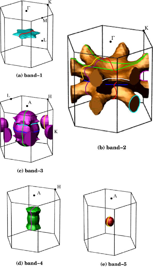
Figure 1: Fermi surfaces generated from the fully itinerant model, which assumes all of the uranium 5f-electrons are included in the Fermi volume. The band 1 and 2 surfaces are hole surfaces; the band 3, 4 and 5 surfaces are electron surfaces. All of the simple extremal orbits on each surface are shown. Table 2 gives the correspondence between these lines and predicted dHvA frequencies of figure 4. On the band 2 surface, the two green lines running across the top indicate possible ‘open orbits’. Note also that subsequent plots are colour coded such that dHvA frequencies thought to arise from a given band are shown in the same colour as the Fermi surface in this figure (e.g. band 2 frequencies will be plotted in brown, etc.)

Taillefer and Lonzarich provided the most direct evidence for the existence of the heavy Fermi liquid, with their measurements of quantum oscillatory magnetization—the de Haas-van Alphen (dHvA) effect [6, 7]. They observed at least five distinct extremal orbits of the Fermi surface, with quasiparticle masses of up to 100 $m_{e}$. All of the observed surfaces could be interpreted by comparison with relativistic band structure calculations [8], which predict the multi-sheeted Fermi surface shown in figure 1. The observed quasiparticle masses were enhanced by between 10 and 20 in comparison with the calculated band mass. Increasing the calculated contribution to $\gamma$ of each Fermi surface sheet by the ratio of the measured to the calculated effective mass gave good agreement with the total measured linear coefficient of the specific heat: that is, these five sheets of the Fermi surface were found to account within error for the observed low temperature linear specific heat coefficient [7]. These dHvA studies of UPt₃, and their interpretation, were very influential in the development of our present understanding of heavy fermion systems, so it is essential to establish them unambiguously, the more so because the interpretation of the dHvA data has recently been called into question by an alternative proposal that two of the uranium $5f$-electrons are localized in UPt₃ [9]. This proposal has the attractive feature that it offers a specific mechanism for producing quasiparticle mass enhancements: the exchange interaction between the itinerant and localized f-electrons. However, this explanation of the mass enhancement is not unique: in addition to the well-established Kondo-lattice mechanism [10, 11] which is believed to explain heavy masses in itinerant 1f cerium heavy fermion compounds, such as CeRu₂Si₂ [12], one can get large mass enhancements from coupling of conduction electrons to their own collective spin-fluctuations [13, 14, 15] as in MnSi (see e.g. [16]). Thus, the argument for adopting the ‘partially localized’ model rests on the claim that it gives a better description of of the Fermi surface than the original ‘fully itinerant’ model. One of the central goals of this paper is to critically examine this claim.

There are other reasons why it is important that we understand the electronic structure of UPt₃. UPt₃ is the archetypal multi-component superconductor (for reviews see references [17, 18]), showing three distinct superconducting phases below $T_{c}\simeq 0.5{\rm\ K}$. It is crucial that the correct Fermi surface be employed in attempting to model thermodynamic measurements in the superconducting state (see e.g. [19]) and that the correct elementary excitations are used in trying to understand the superconducting pairing mechanism: in particular, the symmetry of the pair state will be sensitive to the details of the electronic structure of UPt₃.

From a theory perspective, the nature of the Fermi surface comes to the heart of the debate concerning the behavior of f-electrons in condensed matter systems. Are they localized, itinerant, or is a ‘dual’ model (partially localized and partially itinerant) more appropriate? For instance, in UPd₃, a local-f model gives a good description of the Fermi surface [20], whereas it gives a very poor description of the Fermi surface of UPt₃ [8]. Since UPt₃ sits near the borderline between local and itinerant behavior, it is not a priori clear whether a ‘dual’ or a ‘fully itinerant’ picture is more appropriate.

Finally, there is obvious interest in improving the accuracy of band structure calculations for correlated electron systems, and UPt₃ provides a good test case since it sits very nicely between magnetic d-electron metals, which have fairly broad bands and for which local density approximation (LDA) calculations seem to work well, and more strongly correlated metals, such as sodium cobaltate, in which it is claimed that LDA calculations give an incorrect electronic structure [21].

2 Theoretical models of the Fermi surface

In this paper, the aspect of electronic structure that we focus on is the Fermi surface. Using the Onsager relation (see below) a dHvA oscillation frequency can be convered into a cross-sectional area of a sheet of the Fermi surface that is ‘extremal’ (a maximum or minimum) in the plane perpendicular to the direction of the applied magnetic field. By rotating the crystal in the field the angle dependence of these extremal areas can be followed. It is sometimes possible to derive the shape of the Fermi surface directly from such data, but in practice it is usually necessary to interpret the data by comparison with the Fermi surfaces predicted by band structure calculations. Taillefer and Lonzarich [7] used a Fermi surface generated by Norman et al[8], who calculated the band structure assuming that all the uranium 5f electrons are itinerant (i.e. that the Fermi volume includes these electrons). This Fermi surface, shown in figure 1 together with the path in $k$-space of several of the allowed extremal orbits, was in general agreement with earlier calculations [22, 23, 24], but there are differences in detail. Five bands cross the Fermi energy, and the five panels of figure 1 show the resulting sheets of the Fermi surface: (band 1) a disc-shaped hole surface centred on the $A$ point of the Brillouin zone; (band 2) a multi-connected hole surface centred on $A$ with arms branching out to reach the zone boundary between $L$ and $M$; (band 3) a large $\Gamma$-centred electron surface with subsidiary electron pockets centred at $K$; (band 4) and (band 5) two smaller $\Gamma$-centred electron surfaces.

Table 1: Comparison of notation used for Fermi surfaces of UPt₃: the ‘band number’ is the notation used by Norman et al[8] and in this paper. The other references are: Joynt and Taillefer [17] (a review article on the superconductivity); Taillefer and Lonzarich [7]; Kimura et al[27]; Zwicknagl et al[9]. ‘Colour’ is the colour scheme used to represent a given band on plots of dHvA versus angle.

• Band number	Joynt &	Taillefer &	Kimura	Zwicknagl	Colour
  	Taillefer	Lonzarich	et al	et al
  Band 1	‘Starfish’	Band 5	Band 35	Band 1 (Z1)	Turquoise
  Band 2	‘Octopus’	Band 4	Band 36	—	Brown
  Band 3	‘Oyster &	Band 3	Band 37	Band 2 (Z3)	Purple
  	urchins’
  Band 4	‘Mussel’	Band 2	Band 38	—	Green
  Band 5	‘Pearl’	Band 1	Band 39	Band 2 (Z5)	Red

The notation describing the Fermi surface and dHvA effect in UPt₃ has become rather complicated over the years. In this paper, in keeping with the original notation of Norman et al[8], we are referring to the five bands that cross the Fermi surface as bands 1 through 5, while particular predicted orbits will be labelled by giving the centre of the orbit and the band number. Thus, for example, A-1 is an extremal orbit on band 1, with the orbit centred on the A point in the Brillouin zone (A-1 is indicated by the red line in figure 1(a)). Note, however, that experimentially observed (as opposed to theoretically predicted) dHvA frequencies will be referred to by lower-case Greek letters, following the notation of references [7] and [25, 26, 27]. Different band numbering has been used by different authors, so in table 1 we tabulate the various labelling schemes that have been used, to ease comparison with the published literature.

In [7], agreement between the observed extremal orbits and this calculated Fermi surface was based on a number of points of detail, but rigorous comparison was not possible because quantum oscillations from most Fermi surface sheets were only seen with the field close to the $a$-axis (which corresponds to the $\Gamma-K$ direction in $k$-space), and no oscillations were observed with the field along the $c$-axis (field parallel to $\Gamma-A$). Moreover, some predicted sheets were not observed at all. Many of these gaps were filled by Kimura et al[25, 26, 27], who observed quantum oscillations throughout all three major symmetry planes and along the $c$-axis.

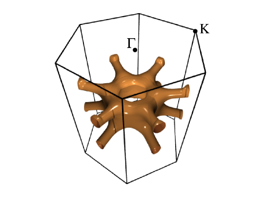
Figure 2: Cartoon of the modified band 2 surface proposed by Kimura et al [25]. The hole through the centre of the surface eliminates the open orbits of figure 1(b).

It has twice been proposed that the Fermi surface shown in figure 1 is wrong. The first proposed change, due to Kimura et al[25], is illustrated in figure 2, where the band 2 surface – in the fully itinerant model a large A-centred hole surface with twelve arms extending to the Brillouin zone boundary – has become a large torus with twelve arms extending to the zone boundary. In this torus geometry there are no ‘open orbits’ on the Fermi surface. (In figure 1(b), the open orbits are shown as green lines running across the top of the Fermi surface, spanning the Brillouin zone.) Such orbits are important in magnetoresistance, because cyclotron motion of quasiparticles arising from the Lorentz force is prevented on open orbits when the applied magnetic field is perpendicular to the orbit: in effect, the quasiparticles on the open orbits, rather than going in circles in both $k$-space, and real space, run along the top of the surface in $k$-space and thus move in roughly a straight line in real space. In copper, for example, this produces very pronounced minima in the high field magnetoresistance when the applied field is perpendicular to the open orbit (see e.g. [28]), and indeed Kimura et aleventually reverted to the original topology of this surface as shown in figure 1(b) [27], largely because the magnetoresistance shows such angular dependent minima, as discussed in more detail below.

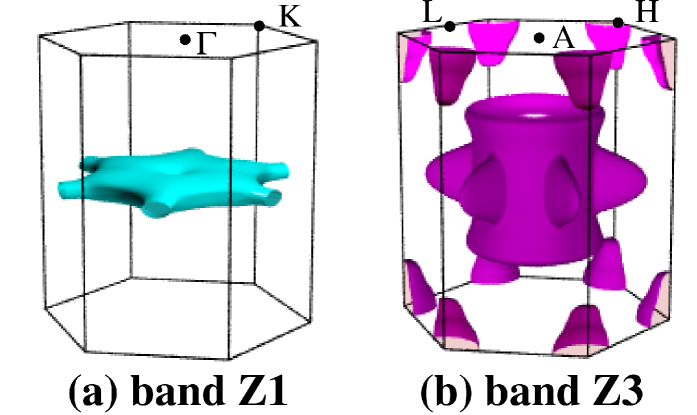
Figure 3: Cartoon representation of the major Fermi surface sheets proposed by Zwicknagl et al[9]. The ‘Z1’ surface has open orbits similar to those of band 2 of the fully itinerant model. The ‘Z3’ surface has a large central electron surface plus small H-centred electron pockets. A small electron surface (Z5), similar to the band 5 surface of the fully itinerant model, is not shown.

The existence of these open orbits is relevant to the more recent, and more radical, proposal by Zwicknagl et al[9] of a dual model for UPt₃, in which two of the three uranium 5f-electrons per formula unit are localized in the sense that they do not contribute to the Fermi volume. We will refer to this as the ‘partially localized’ model, in contrast to the original ‘fully itinerant’ model. Figure 3 shows the Fermi surface for this model. It has two large surfaces, which we label Z1 and Z3 as they seem to correspond most closely to the band 1 and band 3 surfaces of the fully itinerant model, plus a small $\Gamma$-centred electron pocket (not shown).

The band Z1 Fermi surface is similar in shape to the band 1 surface of figure 1(a), however, in the partially localized model it spans the Brillouin zone at the L-points, producing open orbits when the applied field is parallel to the $a$-axis.

The large $\Gamma$-centred electron surface, arising from band Z3, is somewhat larger than, and somewhat different in shape from, the large band 3 surface of the fully itinerant calculation.

The correspondence between the bands should not be taken too literally, as can be understood by examining degeneracies of the bands that arise within the hexagonal close packed crystal structure. (The actual crystal structure of UPt₃ is hexagonal close packed with a slight trigonal distortion [29], but this distortion was not included in the band structure calculations and should have only a tiny effect.) In the hexagonal close packed structure each primitive cell contains two formula units, and thus the bands are related in pairs. These pairs would be degenerate in the A-H-L plane, but this degeneracy is mostly lifted by spin-orbit coupling, leaving only a degeneracy along the A-L lines. It can be seen that in the A–H–L plane the Fermi surfaces of bands 1 and 2 of the fully itinerant model are nearly degenerate, and they are degenerate along the A–L line ; similarly, we see that in the A–H–L plane the H-centred ellipsoids of band Z3 are nearly degenerate with the Z1 surface, implying that these H-centred ellipsoids are the analogue of band 2 of the fully itinerant model; it is only the large $\Gamma$-centred surface of band Z3 that corresponds to band 3, and we also infer that the analogue of band 4 of the fully itinerant model is the small $\Gamma$ surface of the partially localized model (not shown in figure 3). Despite this minor confusion, we will label the H ellipsoids as belonging to ‘Z3’, and the smaller $\Gamma$ surface as belonging to ‘Z5’, as this facilitates comparison of the two models in regards to the dHvA data.

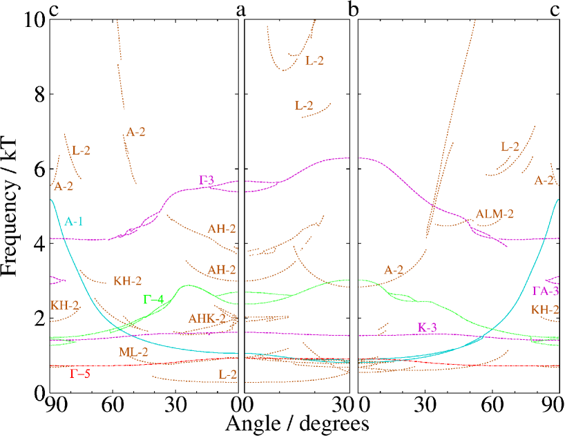
Figure 4: Predicted variation of the dHvA frequency components in the fully itinerant model. The labels give the orbit centre followed by the band number (1–5). Table 2 gives the corresponding orbits in figure 1. At the $c$-axis the applied field is along the hexagonal axis, at $a$ it is parallel to $\Gamma$-K (see figure 1), whereas at $b$ it is parallel to $\Gamma$-M.

It is evident that there are considerable differences between the fully itinerant and partially localized Fermi surfaces, and the main purpose of this paper is to address the controversy over the number of valence f-electrons in UPt₃ by comparing these model Fermi surfaces with experiment. In making this comparison, we make use of the Onsager relation, $F=\hbar A/2\pi e$, which relates an extremal cross-sectional area $A$ of the Fermi surface to the measured dHvA frequency $F$ [30]. Thus, in addition to figures 1 and 3, we show in figures 4 and 5 the variation with angle of the predicted dHvA oscillation frequencies for the fully itinerant model and partially localized models, respectively, extracted from band structures using the Onsager relation. In figure 4 we have included several predicted orbits on the band 2 surface of the fully itinerant model that have not previously been noted. These were obtained using a numerical method that interpolates the eigenvalues of the band structure calculation between $k$ points, locates closed orbits on the Fermi surface (including orbits spanning several Brillouin zones), identifies the extremal (maximum or minimum) orbits and calculates their areas. Table 2 describes these orbits, and gives the correspondence with the orbits drawn on figures 1 and 12.

Most of these ‘new’ orbits are topologically complicated, spanning two or more arms, often non-centrally. For example, AHK-2 circles two arms of band 2 (yellow line in figure 1(b)) and there are two predicted AH-2 orbits that circle four arms of the Fermi surface (purple line in figure 1(b)). A comparison of these orbits with several newly observed Fermi surface branches in our dHvA and Shubnikov–de Haas (sdH) measurements is given in the appendix.

Table 2: Orbits on the fully itinerant model (figure 4), arranged roughly by increasing frequency. The last column gives the proposed correpondence to observed branches of the Fermi surface (see e.g. figure 9)

• Label	Description	Correspondence with figure 1	Assignment
  		figure 1
  L-2	(The lowest frequency) Electron orbit	Purple line on 1(b)	Possibly $\gamma$
  ML-2	Circles one arm on band 2	Turquoise line on 1(b)	$\alpha$
  $\Gamma$-5	Central orbit around band 5 sphere	Yellow line on 1(e)	$\gamma^{\prime}$
  AHK-2	Circles 2 arms	Yellow line on 1(b)	$\eta^{\prime}$
  AH-2	Circles 4 arms	Purple line on 1(b)	$\alpha_{4}^{\prime}$ and $\alpha_{4}$
  $\Gamma$-4	Electron orbit	Red line on 1(d)	$\epsilon$
  KH-2	(At c-axis) Electron orbit	White line on 1(b)	$\zeta$
  K-3	Electron orbit	Yellow line 1(c)	$\kappa$
  KH-2	Near 70o in $c$–$a$ plane	Not shown	$\alpha_{3}$
  A-1	Hole orbit	Red line on 1(a)	$\delta$
  $\Gamma$A-3	Non-central electron orbit	Turquoise line on 1(c)	$\sigma$
  ALM-2	Circles 3 upper arms and one lower	Not shown	$\alpha_{3}$
  A-2	At $b$-axis	Red line on 1(b)	$\lambda$
  A-2	At $c$-axis	Blue line on 1(b)	$\lambda^{\prime}$
  $\Gamma$-3	Electron orbit	Blue line 1(c)	$\omega$
  L-2	High frequency, $a$–$b$-plane	Red line, Figure 12	? $\eta$
  L-2	Higher frequency $a$–$b$-plane	Blue line, Figure 12	$\eta$

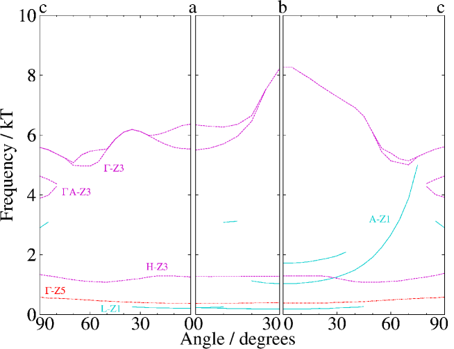
Figure 5: Predicted variation of the dHvA frequency components in the partially localized model. The label indicates the orbit centre and bands (Z1, Z3 and Z5).

In the next section, we describe our experimental results, and then in the discussion we compare our results with the predictions of the fully itinerant and partially localized models.

3 Experimental Results

Quantum oscillation measurements involve considerable technical challenges, especially in the realm of sample preparation because the oscillations are exponentially damped by impurity scattering.

The sample used in our magnetoresistance measurements is a 50 $\mu$m $\times$ 160 $\mu$m $\times$ 4 mm single crystal whisker, produced by quenching a stoichiometric melt in ultra-high vacuum. The whisker was annealed near its melting temperature ($\sim 1700^{\rm o}$C) for a short time, then near 1400^oC for several hours, and finally overnight at 1200^oC. The residual resistivity of this sample was 0.03 $\mu\Omega$ cm, at least a factor of two better than a whisker crystal in which Taillefer and Lonzarich had previously observed weak quantum oscillations in the magnetoresistance [31], and roughly 10 times better than that of a sample used by Kimura et al [25] in their first study of the angular dependence of the magnetoresistance.

Magnetoresistance measurements were made by a standard four-terminal technique, with the current along the $c$-axis, and the field in the basal plane. Typical currents were 1 to 10 $\mu$A.

The sample used in the dHvA oscillation measurements was grown in Grenoble by Czochralski pulling from a water cooled copper crucible, using high purity starting materials. The sample was annealed for 7 days at 950^o C under UHV. With the current in the $a$-direction the RRR was 283 (not extrapolated to $T=0$), and $T_{c}$ was 540 mK, with a width of 8 mK.

All measurements were carried out in a specially designed cryomagnetic facility, which has an 18 tesla superconducting magnet, modulation coils which can supply up to 0.02 T at 20 Hz with the magnet at 18 T, a top-loading dilution refrigerator with a base temperature of 6 mK, and an externally controlled rotation stage which allows the angle between the applied field and the symmetry axes of the crystal to be varied. The quantum oscillatory magnetization was measured in a standard way, with the sample placed in one coil of a copper-wire astatic pair. The modulation field was typically 0.01 T at 2 Hz, the low frequency being used in order to minimize eddy current heating.

The interpretation of quantum oscillations in strongly correlated electron systems has recently been reviewed [30, 32]. Briefly, thermodynamic and transport properties oscillate as a function of applied field $B$ due to passage through the Fermi surface of quantized cyclotron orbits (called Landau levels) of charged fermion quasiparticles. Each measured oscillation frequency $F$ is related to an extremal Fermi surface area $A$ (measured perpendicular to the applied field) by the Onsager relation $F=\hbar A/2\pi e$. Quantum oscillations are only seen if the width of the Fermi distribution is narrow compared with the Landau level spacing, so the oscillations are only seen at low temperature: in the measurements described here the temperature was typically below 30 mK.

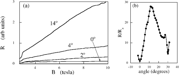
Figure 6: (a) Resistivity versus field for various in-plane angles between the field and the $a$-axis. The very weak magnetoresistance when the field is aligned with the $a$-axis ($0^{\rm o}$ line) is strong evidence for an open orbit. (b) Resistivity versus angle at 8 T and 20 mK, showing the sharp dips with the field along the $a$ ($0^{\rm o}$) and $b$ ($30^{\rm o}$) axes.

Our results for the transverse dc-magnetoresistance (i.e. the non-oscillatory magnetoresistance) are illustrated in figure 6, which shows the field dependence of the $c$-axis resistivity at 20 mK for four different orientations of the applied field, and the variation of the $c$-axis resistivity at $B=8$ T as the field is rotated within the basal plane. The strong angle dependence seen in our results contrasts sharply with [25, 26] where only extremely weak anisotropy was found in the basal-plane magnetoresistance, but it is in excellent agreement with Taillefer et al [33] and reference [27]. Indeed, we see stronger angle dependence than in previous work, an indication of improved sample quality.

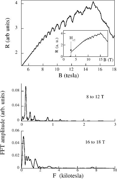
Figure 7: The quantum oscillatory magnetoresistance in our high purity whisker crystal of UPt₃, with the field applied in the basal plane about 8^∘ from the $b$-axis, and the current along $c$. The most prominent oscillations correspond to a previously unobserved frequency. The upper plot shows a complete trace in the inset, taken at 20 mK, whereas the main plot focuses on the oscillations. The middle plot is a quantum oscillation spectrum obtained from the data between 8 and 12 T by interpolating it at equally spaced intervals in $1/B$ and taking the fast Fourier transform. The largest peak, at 0.14 kT, is the new frequency, and it is labelled $\gamma^{\prime}$ in figures 9 and 10. The bottom plot is the quantum oscillation spectrum from the data between 16 and 18 T. The peak at 7.5 kT is also a previously unobserved frequency, labelled $\eta$ in figures 9 and 10.

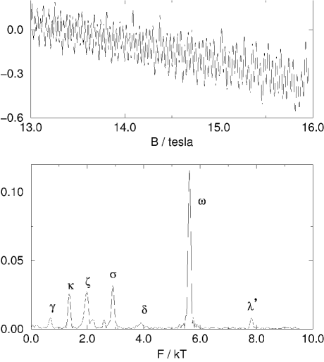
Figure 8: Typical oscillatory variation of the dHvA magnetization as seen at 10 mK with the applied field directed approximately 5^∘ from the $c$-axis towards the $b$-axis (upper trace) and corresponding Fourier spectrum (lower trace). The peaks are labelled according to our assigment on the rotation plots (see figure 9).

Quantum oscillations in the magnetoresistance of our single crystal whisker, with the magnetic field applied in the basal plane, are shown in figure 7, together with the amplitude spectra over two field ranges: from 8 to 12 T, and 16 to 18 T. Figure 8 shows typical quantum oscillatory magnetization for the Grenoble single crystal, detected at the second harmonic of the modulation frequency, and taken with the magnetic field aligned close to the $c$-axis.

Scans such as those shown in figures 7 and 8 were repeated at many angles, with the oscillatory magnetoresistance measurements focused on the $a$–$b$-plane, while the dHvA measurements were done only in the $a$–$c$- and $b$–$c$-planes, with somewhat stronger focus on the $b$–$c$-plane and with the crystals oriented so that signals were strongest near the $c$-axis. Field sweeps were typically divided into two ranges, from 8 to 12 T, and 14 to 18 T. The results are summarized in figure 9, which shows the fundamental dHvA frequencies versus angle for the three major symmetry planes.

The data of figure 9 have been ‘cleaned’ to eliminate higher harmonic frequencies and occasional isolated points. We have included the results of Taillefer and Lonzarich [7], which are in excellent agreement with ours, and which are complimentary in the sense that their dHvA studies of the $a$–$c$- and $b$–$c$-planes saw oscillations only at low angles (close to $a$ and $b$), whereas our dHvA results are best close to the $c$-axis due to the configuration of our pickup coils. In comparing our results with the theory this limitation should be kept in mind, and it probably explains why, for example, we see branches that may correspond to AH-2 in the $a$–$b$-plane where the SdH oscillations were very strong, but we don’t see them near the $a$ axis in the $a$–$c$-plane, where our dHvA signals were comparatively weak.

Like Kimura et al [25, 26, 27], we were able to follow many branches to the $c$-axis, and in general our results are in good agreement with theirs, but in addition we observe a number of new frequencies.

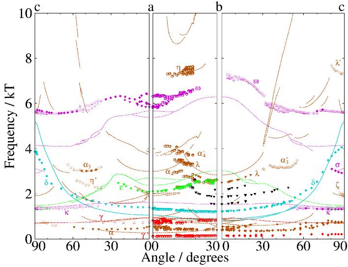
Figure 9: Angle dependence of measured quantum oscillation frequencies. The lines are the predictions of the fully itinerant model. The colour code reflects our band assignments as in figure 1 (e.g. light blue is for frequencies arising from band 1, brown from band 2, etc). Black symbols are believed to be so-called breakdown orbits in which the quasiparticles tunnel between bands 1 and 2 as they undergo cyclotron motion [7]. Triangles are the data of Taillefer and Lonzarich [7], circles are from our quantum oscillatory magnetoresistance measurements (e.g. figure 7), filled diamonds are low-field (8–12 T) dHvA data, pentagons are from high-field (14–18 T) dHvA data.

The Greek letters in figure 9 follow [7, 27] with additions for new orbits. We have observed nine new orbits in all, which we have labelled $\lambda^{\prime},\ \alpha_{3},\ \alpha_{3}^{\prime},\ \alpha_{4},\ \alpha_{4}^{\prime},\ \kappa,\ \gamma^{\prime},\ \zeta,\ \eta,\ \eta^{\prime}$. Athough effective masses are not the focus of this paper, in table 3 we give the masses, and the calculated band masses (assuming that the fully itinerant model is correct), for these new orbits.

Table 3: Measured effective mass and calculated band mass from the fully itinerant model for newly observed dHvA orbits.

• Orbit	Plane	$m^{*}/m_{e}$	$m_{band}/m_{e}$	Fully itinerant model frequency
  $\kappa$	($c$–$a$) and ($b$–$c$)	$70\pm 10$	3.5	K-3, at $c$-axis
  $\eta$	($a$–$b$)	$130\pm 20$	13.0	L-2 (high frequency), 15o from $a$ in $a$—$b$-plane
  $\alpha^{\prime}_{4}$	($a$–$b$)	$110\pm 30$	8.0	AH-2 (upper branch), 10o from $a$ in $a$–$b$-plane
  $\alpha_{4}$	($a$–$b$)	$80\pm 20$	4.2	AH-2 (lower branch), 10o from $a$ in $a$–$b$-plane
  $\lambda^{\prime}$	($b$–$c$)	$70\pm 5$	4.8	A-2, at $c$-axis
  $\alpha^{\prime}_{3}$	($b$–$c$)	$55\pm 5$	7.7	ALM-2, 50o from $b$
  $\zeta$	($b$–$c$)	$70\pm 15$	2.8	KH-2, at $c$-axis
  $\gamma^{\prime}$	($a$–$b$) and ($b$–$c$)	$16\pm 3$	1.9	$\Gamma$-5, 10o from $a$ in $a$–$b$-plane

An additional important difference from previous studies is that we have followed the $\delta$ orbit all the way to the c-axis, whereas previously it had only been followed to within about 20^∘ of $c$. The significance of this is discussed below.

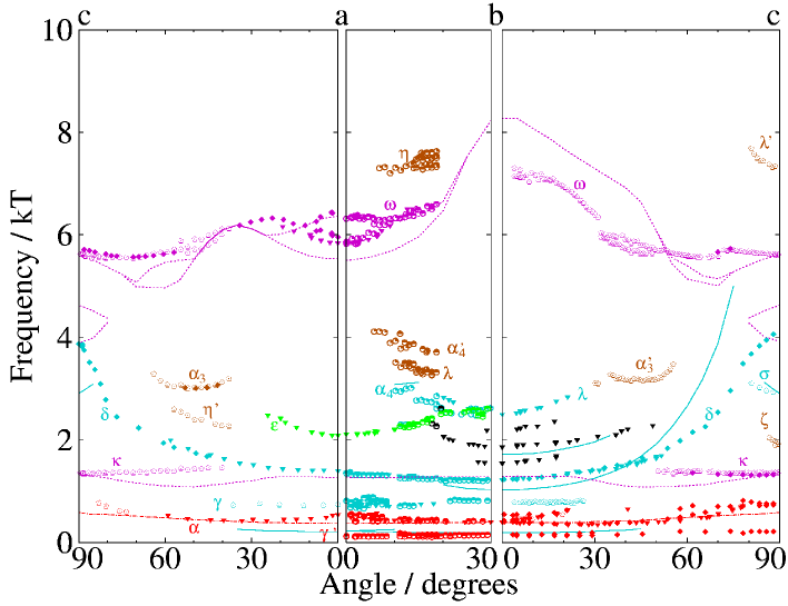
Figure 10: Comparison between measured quantum oscillation frequencies (same data as figure 9) and the predictions of the partially localized model (solid lines).

The lines on figure 9 are the predictions of the fully itinerant model (as per figure 4), and in the subsequent figure, figure 10, we show the data together with the predictions of the partially localized model (figure 5). In the next section, we carry out a detailed comparison between the data and the predictions of the models.

4 Discussion

The extreme angle dependence of the dc-magnetoresistance, shown in figure 6, can be explained following Taillefer et al[33] who argue that it arises from canonical $\omega_{c}\tau>1$ effects. They point out (a) that the large magnetoresistance seen at most angles is indicative of an open orbit, since UPt₃ is compensated and therefore ought not to have a magnetoresistance unless there are open orbits, and (b) that the low magnetoresistance with the field along the $a$-axis is plausibly explained if the open orbit spans the arms of the band 2 surface, as shown in figure 1(b). Within this explanation, in [25] a strongly anisotropic magnetoresistance was not seen because their measurement was made at too high a temperature and in a lower quality crystal, so that the $\omega_{c}\tau>1$ condition was not reached. (To observe an open orbit in the magnetoresistance, the quasiparticle mean free path must be at least long enough that quasiparticles, driven by the Lorentz force, can cross the Brillouin zone before they scatter.) Similarly, the reason we see a stronger magnetoresistance than Taillefer et al[33] is because our sample is purer, and so has a larger value of $\omega_{c}\tau$. The $\omega_{c}\tau$ interpretation is further supported by Taillefer et al[3], who show that the transverse magnetoresistance, with $B$ lying between the $a$- and $b$-axes, rises dramatically only at temperatures below 0.6 K, that is, when the Fermi liquid thermal scattering rate falls below $\omega_{c}$, as expected from an $\omega_{c}\tau>1$ effect.

We note that, if the dip in the magnetoresistance at $B\parallel a$ shows that an open orbit runs diagonally across the band A-2 surface from one arm to the other, then the dip at $b$ appears to suggest a second open orbit, possibly running non-centrally along the top of the band 2 surface. We have also indicated this possible open orbit in figure 1(b).

Within the fully itinerant picture there is thus excellent agreement between the topology of the band 2 surface and the angle dependence of the magnetoresistance. However, the Z1 Fermi surface in the partially localized model also has open orbits, very similar to those of the band 2 surface of the fully itinerant model, so the angle-dependent magnetoresistance alone does not discriminate between these models. However, the existence of these open orbits must be kept in mind in considering any fine-tuning of the partially localized model that will be required to obtain agreement with the quantum oscillation data.

Turning to the quantum oscillations, we firstly note that there are major differences in the predictions of the fully itinerant and partially localized theories. At the coarsest level of comparison, it is evident that the partially localized model predicts many fewer dHvA frequencies than does the fully itinerant model. This mostly reflects the absence in the partially localized model of a surface corresponding to the band 2 ‘octopus’, as this surface generates many orbits in the fully itinerant model.

It is at this coarsest level of comparison that the deficiencies of the partially localized model are perhaps most evident, because it simply predicts many fewer dHvA orbits than are actually observed. The frequencies labelled $\alpha$, $\alpha_{3}$, $\alpha_{3}^{\prime}$, $\alpha_{4}^{\prime}$, $\eta$, $\eta^{\prime}$, $\zeta$, $\lambda$, $\lambda^{\prime}$ and $\epsilon$ find no explanation in the partially localized model, nor do the three frequencies between 1.5 and 2.5 kT near the $b$-axis, ascribed in [7] to breakdown orbits between the band 1 and band 2 surfaces of the fully itinerant model. Also, the $\delta$ oscillation, arising from band 1/Z1, is clearly observed in the data to extend across the $a$–$c$-plane, whereas in the partially localized model it should not appear in this plane at all, due to the open orbits on the Z1 surface.

We can understand the nature of these deficiencies better via a more detailed level of quantitative, band-by-band comparison.

Starting with band 3/Z3 – the largest, most thermodynamically relevant, sheet of the Fermi surface – as pointed out by Zwicknagl et al[9], the Z3 surface is in better quantitative agreement with the $\omega$ orbit than is the band 3 sheet of the fully itinerant model. It is on this basis that Zwicknagl et al [9] claimed that the partially localized model is superior. If the fully itinerant band 3 surface is to be brought into agreement with the data it has to be increased in size: the angle dependence follows that of the data quite well, however.

Bands 3/Z3 both have, as well as the large $\Gamma$-centred surfaces, smaller, roughly spherical sufaces of similar size, but located at different points of the Brillouin zone: in the fully itinerant model there are $K$-centred ellipsoids as shown in figure 1(c). The partially localized model in contrast has $H$-centred ellipsoids, but of almost exactly the same size. The branches which we have labelled $\kappa$ in figures 9 and 10 could arise from either of these surfaces (see the branches labelled K-3 and H-Z3 in figures 4 and 5). This is a very weak oscillation in our data, not previously observed. One issue with an assignment to K-3 is that increasing the size of the band 3 $\Gamma$ surface as discussed in the previous paragraph would also cause the $K$-centred pockets to increase, as they are also electron-like. In fact, one problem with the fully itinerant  model is that to increase the size of the $\Gamma$ surface to agree with experiment, one has the danger that this surface merges with the $K$-centred ellipsoids. To correct for this would require a distortion in the dispersion of this band. Note, however, that, as discussed below, these $\kappa$ oscillations could also arise from the band 4 surface of the fully itinerant model.

Turning next to band 1/Z1 (the $\delta$ branch) the partially localized model gives the best prediction of the quantitative value of this frequency at the $b$-axis, however, only the fully itinerant model correctly predicts: (1) that this oscillation spans the entire $a$–$b$-plane, (ii) that it will be seen in the $a$–$c$-plane, and (iii) that it will extend to the $c$-axis in both the $a$–$c$- and the $b$–$c$-planes. These discrepancies between the partially localized model and the data were not addressed by Zwicknagl et al[9], yet it categorically shows that the topology of the Z1 surface is wrong: this surface is closed (i.e. it cannot have arms extending to the zone boundary) in contrast to figure 3(a). Yet, as noted above, open orbits are required in order to explain the angle dependence of the magnetoresistance. Only by introducing an additional Fermi surface with open orbits, and adjusting the Z1 surface so that it is closed, can the partially localized model be brought into agreement with both the angle dependence of the $\delta$ oscillation and the angle dependence of the magnetoresistance. It is thus clear that not only is the Z1 topology wrong, there is also a major missing Fermi surface in the partially localized model.

Band-2 of the fully itinerant model has open orbits, as shown in figure 1(b), that explain the angle dependence of the magnetoresistance. It was found in previous studies to provide a natural explanation of the $\alpha$ and $\lambda$ oscillations. However, these find alternative explanations in the partially localized model: the $\lambda$ oscillation follows the angle dependence of a non-central orbit on the Z1 surface, as illustrated in figure 10, while $\alpha$ could be explained by either $\Gamma$-Z5 or L-Z1. However, we believe that several of our new frequencies provide unambiguous evidence for the existence of the band 2 surface: the $\lambda^{\prime}$ orbit finds a natural interpretation in the fully itinerant model as the orbit encircling the ‘waist’ of this surface when the field is parallel to $c$ (this is the blue line in figure 1(b)), although the frequency is slightly larger than that predicted. This very clear frequency (shown in figure 8) has not been previously reported. We found that it has a high mass: $70\pm 5m_{e}$. We note that Kimura et al [25] also believed that they had found this orbit, which they called $\tau$, but it was at a lower frequency, and we did not observe this signal at all. We believe that our $\lambda^{\prime}$ frequency is in better agreement with the overall size of the band 2 surface. We note additionally that the $\eta$, $\eta^{\prime}$, $\alpha_{3}^{\prime}$, $\alpha_{4}$ and $\alpha_{4}^{\prime}$ frequencies are only explainable via the topologically complicated orbits on the band 2 surface, and not within the partially localized model, as shown in figure 11. This is discussed further in the appendix, but we draw attention particularly to the $\eta$ orbit, a strong, high frequency oscillation in the basal plane, that corresponds well to non-central orbits that span two Brillouin zones, as illustrated in figure 12.

Final, circumstantial evidence in favour of the existence of the band 2 surface is that it makes a major (roughly 30%) contribution to the linear coefficient of specific heat, and if it does not exist then the linear coefficient of the specific heat is no longer explained by the quasiparticle masses.

It thus seems very likely that it is this Fermi surface which is missing from the partially localized model.

The $\epsilon$ orbit has previously been assigned to band 4 in the fully itinerant model, i.e. $\Gamma$-4 [7], but it was not clear why this oscillation was only seen near the basal plane when it should be seen at all angles. A second possible interpretation of our $\kappa$ oscillation is that it is the extension of this oscillation, but if this is true then the $K$-centred orbits of band 3 either do not exist, or their oscillations are even weaker than these signals.

Finally, turning to band 5, one of the mysteries of previous studies is why this small electron sheet, with orbit $\Gamma$-5, does not show up more clearly. Taillefer and Lonzarich [7] assigned it to a frequency of about 0.7 kT near the $a$-axis with the field in the basal plane. We see a corresponding frequency extending toward the $c$-axis in the $a$–$c$-plane, within about 30^∘ of the basal plane, but the signal then disappears abruptly, which is not easily explained for a simple spherical surface.

A new candidate for this surface is, however, the strong low-frequency signal seen in the magnetoresistance (the most visible oscillation in figure 7), with a frequency between 0.1 and 0.2 kT, labelled $\gamma^{\prime}$ in figure 9. Although it is very strong in the magnetoresistance, it has not been previously reported, presumably because low frequencies are much harder to see in dHvA. We believe that the surface which gives rise to this oscillation is roughly spherical, because we were eventually able to follow it in dHvA measurements toward the $c$-axis in the $b$–$c$-plane, although we did not observe it along the $c$-axis, nor in the $a$–$c$-plane. The amplitude of this oscillation in the magnetoresistance is really huge (see figure 7), given the small size of the Fermi surface, and it is also strongly angle-dependent The signal is strongest when the field is in the basal plane about 10^∘ from $b$: in this angular region, the non-oscillatory magnetoresistance has a shoulder (see figure 6). We have no explanation of the strength of this SdH oscillation; sometimes magnetoresistance oscillations from small surfaces can be strong if the surface acts as an ‘interferometer’ for larger Fermi surfaces [28], but we do not have a model for such an interferometer in the Fermi surface shown in figure 1. If indeed these oscillations arise from $\Gamma$-5, then the surface in the fully itinerant calculation is too large. The quasiparticle mass on this surface was measured to be 16 $\pm$ 3 $\rm m_{e}$.

Finally, we note that the original fully itinerant model, while generally in much better agreement with the data, still has quantitative discrepancies with the data that are at least as striking as those that have recently aroused interest in sodium cobaltate [21]. Although it seems unlikely that better Fermi surface measurements will soon be on the horizon for UPt₃, it may be that the present data set is sufficiently detailed that it could be used as the basis for improving electronic structure methods for f-electron systems. For instance, it would be interesting if the Fermi surface of UPt₃ could be calculated from dynamical mean field theory, as this technique has shown recent promise in other actinide materials such as plutonium [34].

5 Conclusions

The Fermi surface of UPt₃ has over the past two decades been experimentally determined to a high degree of accuracy, allowing comparison with the results of electronic structure calculations at both coarse and fine levels of detail. Our new results fill some gaps in earlier data, and serve to emphasize the rather large number of Fermi surfaces of the heavy fermion state of UPt₃, and the topological complexity of some of the surfaces.

We find that the partially localized model, which assumes that two 5f-electrons per uranium atom are localized, shows unacceptably large discrepancies with observations. Although it gives good agreement with the large electron sheet, and some other oscillations, it has grave difficulty in explaining many of the observed oscillations. At the crudest level, there are a lot more oscillations present than can be supported on the partially localized Fermi surface. At a deeper level, the topology for the band Z1 surface does not agree at all well with the dHvA data, and if it is modified to agree, then one can no longer explain the angle dependence of the magnetoresistance. It is clear that a major, experimentally observed, sheet of the Fermi surface is missing from the partially localized model. We have argued that the band 2 Fermi surface of the fully itinerant model must be close to the shape of this ‘missing’ Fermi surface, and thus that the fully itinerant model of the Fermi surface provides a much better explanation of the data: thus we conclude that, on the basis of existing band-structure calculations, the experimental evidence very strongly favours the model in which all three of the uranium f-electrons are delocalized in UPt₃.

6 Acknowlegement

This work has been supported by the US DOE, Office of Science, under contract no. DE-AC02-06CH11357, the Natural Science and Engineering Research Council of Canada, the Canadian Institute for Advanced Research, and the Engineering and Physical Science Research Council of the UK.

7 Appendix. Assignment of band 2 orbits

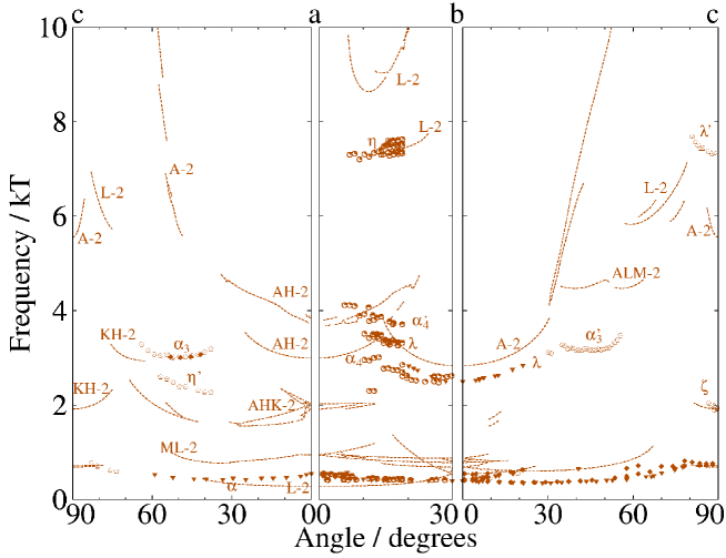
Figure 11: Angle dependence of frequencies ascribed to band 2 in the fully itinerant model.

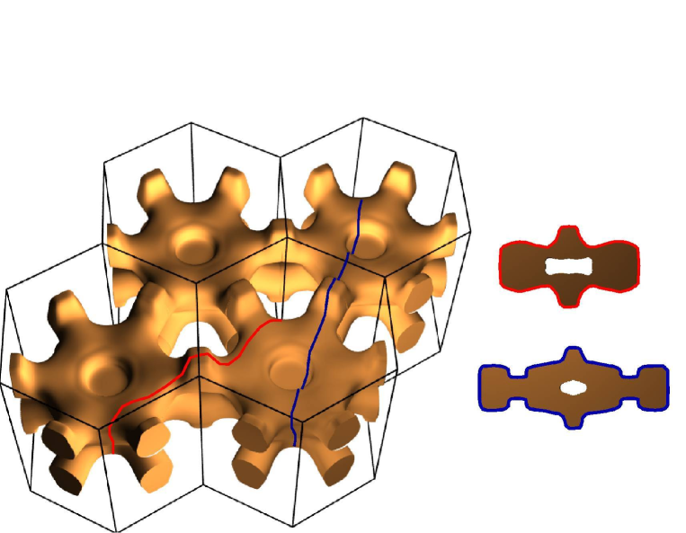
Figure 12: The L-2 frequencies that lie between 6.0 and 10.0 kT between $a$ and $b$ span two Brillouin zones. The main figure shows these orbits projected on the band 2 Fermi surface in the extented zone scheme, while the right shows the cross sections in cut-away view. The lower of the two frequencies, outlined in red, is only marginally extremal: small shifts in the Fermi surface would eliminate this as an extremal orbit. The higher frequency, shown in blue, is much more robust, extends over a greater range of angles, and is thus more likely to correspond to our $\eta$ frequency.

In this paper, a number of new quantum oscillation orbits are described, but we did not assign them to specific predicted orbits in the fully itinerant model because the case for preferring that model to the partially localized model can be made without resorting details. Nevertheless, it is possible to explain our new orbits using the band 2 surface (with the exception of $\gamma^{\prime}$, which we have ascribed to the $\Gamma$-5 orbit).

Figure 11 shows the angle dependence of dHvA frequencies for the band 2 surface (solid lines) from the fully itinerant model compared with observed oscillation frequencies that we have ascribed to this surface.

Recall that our two labelling systems are: for the theoretical prediction, letters and numbers identify the centre of the orbit in $k$-space and the band on which the orbit exists; for the experimental observation we use lowercase Greek letters.

The following assignments had been made previously: $\lambda$ is assigned to A-2, the orbit that circles the body of band 2 (red line in figure 1(b)); $\alpha$ is assigned to ML-2, the orbit that encircles one arm of band 2 (turquoise line in figure 1(b)) [7].

Our best assignment of the ‘new’ orbits is: $\alpha_{4}$ and $\alpha_{4}^{\prime}$ correspond to the two AH-2 orbits, which both circle four arms but at different distances out from the centre of the surface (purple line in figure 1(b)); $\eta$ seems to agree well with L-2, which is the red orbit in figure 12 which spans two zones, however, this orbit is only marginally extremal, so it might be better to ascribe this frequency to the larger, but more stable, orbit shown by the blue line on figure 12 – this orbit is also labelled L-2 and it too spans two Brillouin zones; $\alpha_{3}$ corresponds well to KH-2, while $\alpha_{3}^{\prime}$ corresponds (not quite so well) to ALM-2, both of which circle three upper arms and one lower arm when the field is at a rather high angle going towards $c$ (these orbits are not shown on figure 1(b)); $\eta^{\prime}$ corresponds well to AKH-2, the orbit that circles two arms (yellow line on figure 1(b)); $\zeta$ corresponds well to KH-2, which is an electron orbit that runs around the interior of the arms of three adjacent Brillouin zones (white line in figure 1(b)); and we believe that $\lambda^{\prime}$ is, as discussed in the text, the central orbit that runs around the waist of band 2 (blue line in figure 1(b)).

The comparison between the newly observed orbits and the predictions for this surface is, we believe, very convincing, keeping in mind that there were some limitations to our experiment: our dHvA signals were comparatively weak near the $a$–$b$-plane because of the orientation of the crystal in the pickup coils. Thus, the failure to see the AH-2 and the AHK-2 orbits near the $a$-axis in the $a$–$c$-plane is understandable, if unfortunate. Moreover, the quantum oscillatory magnetoresistance, which gave rise to the oscillations between 3.0 and 4.0 kT in the $a$–$b$-plane, lost intensity near the $a$-axis due to the near-vanishing of the magnetoresistance there; hence these oscillations could not be followed to the $a$-axis in the $a$–$b$-plane either.

Thus, the best regions for comparison are close to the $c$-axis in the $a$–$c$- and $b$–$c$-planes, and at intermediate angles in the $a$–$b$-plane, and this is precisely where we find many oscillations that are only explainable by band 2 of the fully itinerant model.

References

References

- [1] P. H. Frings, J. J. M. Franse, F. R. de Boer and A. Menovsky, J. Magn. Magn. Mater. 31-34 (1983) 240.
- [2] G. R. Stewart, Z. Fisk, J. O. Willis and J. L. Smith, Phys. Rev. Lett. 52 (1984) 679.
- [3] L. Taillefer, F. Piquemal and J. Flouquet, Physica C 153-155 (1988) 451.
- [4] F. Marabelli, P. Wachter and J. J. M. Franse, J. Magn. Magn. Mater. 63 & 64 (1987) 377.
- [5] N. Bernhoeft and G. G. Lonzarich, J. Phys.: Condens. Matter 7 (1995) 7325.
- [6] L. Taillefer, R. Newbury, G. G. Lonzarich, Z. Fisk and J. L. Smith, J. Magn. Magn. Mater. 63 & 64 (1987) 372.
- [7] L. Taillefer and G. G. Lonzarich, Phys. Rev. Lett. 60 (1988) 1570.
- [8] M. R. Norman, R. C. Albers, A. M. Boring and N. E. Christensen, Solid State Comm. 68 (1988) 245.
- [9] G. Zwicknagl, A. N. Yaresko and P. Fulde, Phys. Rev. B 65 (2002) 081103(R).
- [10] A. Auerbach and K. Levin, Phys. Rev. Lett. 57 (1986) 887.
- [11] A. J. Millis and P. A. Lee, Phys. Rev. B 35 (1987) 3394.
- [12] H. Aoki, S. Uji, A. K. Albessard and Y. Onuki, J. Phys. Soc. Japan 61 (1992) 3457.
- [13] G. G. Lonzarich and L. Taillefer, J. Phys. C: Solid State Phys. 18 (1985) 4339.
- [14] M. R. Norman, Phys. Rev. Lett. 59 (1987) 232.
- [15] T. Moriya and T. Takimoto, J. Phys. Soc. Japan 64 (1995) 960.
- [16] G. G. Lonzarich, J. Magn. Magn. Mater. 76–77 (1988) 1.
- [17] R. Joynt and L. Taillefer, Rev. Mod. Phys. 14 (2002) 235.
- [18] J. A. Sauls, Adv. Phys. 43 (1994) 678.
- [19] M. R. Norman and P. J. Hirschfeld, Phys. Rev. B 53 (1996) 5706.
- [20] M. R. Norman, T. Oguchi and A. J. Freeman, J. Magn. Magn. Mater. 69 (1987) 27.
- [21] H.B. Yang, Z.H. Pan, A.K.P. Sekharan, T. Sato, S. Souma, T. Takahashi, R. Jin, B.C. Sales, D. Mandrus, A.V. Fedorov, Z. Wang, H. Ding, Phys. Rev. Lett. 95 (2005) 146401.
- [22] T. Oguchi and A. J. Freeman, J. Magn. Magn. Mater. 52 (1985) 174.
- [23] C. S. Wang, M. R. Norman, R. C. Albers, A. M. Boring, W. E. Pickett, H. Krakauer and N. E. Christensen, Phys. Rev. B 35 (1987) 7260.
- [24] M. R. Norman, T. Oguchi and A. J. Freeman, Phys. Rev. B 38 (1988) 11193.
- [25] N. Kimura, R. Settai, Y. Onuki, H. Toshima, E. Yamamoto, K. Maezawa, H. Aoki and H. Harima, J. Phys. Soc. Japan 64 (1995) 3881.
- [26] N. Kimura, R. Settai, Y. Onuki, K. Maezawa, H. Aoki and H. Harima, Physica B 216 (1996) 313.
- [27] N. Kimura, T. Komatsubara, D. Aoki, Y. Onuki, Y. Haga, E. Yamamoto, H. Aoki and H. Harima, J. Phys. Soc. Japan 67 (1998) 2185.
- [28] A. B. Pippard, Magnetoresistance in Metals, Cambridge University Press, 1989.
- [29] D. A. Walko, J.-I. Hong, Rao T. V. Chandrasekhar, Z. Wawrzak, D. N. Saidman, W. P. Halperin and M. J. Bedzyk, Phys. Rev. B 63 (2001) 054522.
- [30] D. Shoenberg, Magnetic Oscillations in Metals, Cambridge University Press, 1984.
- [31] L. Taillefer and G. G. Lonzarich, unpublished.
- [32] A. Wasserman and M. Springford, Adv. Phys. 45 (1996) 471.
- [33] L. Taillefer, J. Flouquet and W. Joss, J. Magn. Magn. Mater. 76 & 77 (1988) 218.
- [34] J. H. Shim, K. Haule and G. Kotliar, Nature 446 (2007) 513.