Conformal Invariance of Iso-height Lines in two-dimensional KPZ Surface

Abstract

The statistics of the iso-height lines in (2+1)-dimensional Kardar-Parisi-Zhang (KPZ) model is shown to be conformal invariant and equivalent to those of self-avoiding random walks. This leads to a rich variety of new exact analytical results for the KPZ dynamics. We present direct evidence that the iso-height lines can be described by the family of conformal invariant curves called Schramm-Loewner evolution (or $SLE_{\kappa}$) with diffusivity $\kappa=8/3$. It is shown that the absence of the non-linear term in the KPZ equation will change the diffusivity $\kappa$ from $8/3$ to $4$, indicating that the iso-height lines of the Edwards-Wilkinson (EW) surface are also conformally invariant, and belong to the universality class of the domain walls in the O(2) spin model.

Recently, it was shown that the statistics of the zero-vorticity lines in inverse cascade of two dimensional (2D) Navier-Stokes turbulence is conformally invariant and belongs to the percolation universality class bernard1 . The same issue has been studied for zero-temperature isolines in the inverse cascade of surface quasigeostrophic turbulence bernard2 , domain walls of spin glasses spin glass and the nodal lines of random wave functions Keatin . Moreover, it has been shown recently that the statistics of the iso-height lines on the experimental $WO_{3}$ grown surface is the same as domain walls statistics in the critical Ising model as well as those of Ballistic Deposition (BD) model WO3 .
Evidence of conformal invariance in the geometrical features of such complex nonlinear systems have been provided, in the continuum limit, by stochastic (Schramm) Loewner evolution, i.e., $SLE_{\kappa}$, where $\kappa$ is the diffusivity schramm ; cardy . Schramm and Sheffield showed that the contour lines in a two-dimensional discrete Gaussian free field are statistically equivalent to $SLE_{4}$ Schramm-Sheffield . Moreover, it is shown that the restriction property only applies in the case for $\kappa=8/3$ Schramm-Lawler . Since self-avoiding random walk (SAW) satisfies the restriction property, it is conjectured in the scaling limit to fall in the SLE class with $\kappa=8/3$ Tom-Kennedy . The scaling limit of SAW in the half-plane has been proven to exist G. Lawler but there is no general proof of its existence.

In this Letter we investigate numerically the iso-height lines of the (2+1)-dimensional Kardar-Parisi-Zhang (KPZ) model Kardar , and study their possible conformal invariance. It is shown that the KPZ’s iso-height lines are equivalent to self-avoiding walks, and that the iso-height lines in the 2D-KPZ surface are $SLE_{8/3}$ curves. For the Edwards-Wilkinson (EW) interface (the KPZ model without the nonlinear term) the iso-height lines fall in the universality class of the interfaces in the $O(2)$ model, and can be described by $SLE_{4}$.

The KPZ equation is given by

$$\frac{\partial h(\textbf{x},t)}{\partial t}=\nu\nabla^{2}h+\frac{\lambda}{2}\mid\nabla h\mid^{2}+\eta(\textbf{x},t)\;.$$ (1)

The first term on the r.h.s describes relaxation of the interface caused by a surface tension $\nu$, and the nonlinear term is due to the lateral growth. The noise $\eta$ is uncorrelated Gaussian white noise in both space and time with zero average i.e., $\langle\eta(\textbf{x},t)\rangle=0$ and $\langle\eta(\textbf{x},t)\eta(\textbf{x}^{\prime},t^{\prime})\rangle=2D\delta^{d}(\textbf{x}-\textbf{x}^{\prime})\delta(t-t^{\prime})$. The KPZ equation is invariant under translations along both growth direction and perpendicular to it, as well as time translation and rotation stanley . Rescaling the variables, $h=\tilde{h}\sqrt{2D/\nu}$, and $t=\tilde{t}/\nu$, changes Eq. (1) to, $\partial\tilde{h}(\textbf{x},\tilde{t})/\partial{\tilde{t}}=\nabla^{2}\tilde{h}+\sqrt{\epsilon}\mid\nabla\tilde{h}\mid^{2}+\tilde{\eta}(\textbf{x},\tilde{t})$, where $\epsilon=\lambda^{2}D/2\nu^{3}$ and $\langle\tilde{\eta}(\textbf{x},\tilde{t})\tilde{\eta}(\textbf{x}^{\prime},\tilde{t}^{\prime})\rangle=\delta^{d}(\textbf{x}-\textbf{x}^{\prime})\delta(\tilde{t}-\tilde{t}^{\prime})$. In the following, we work with the single parameter $\epsilon$ and drop all the tildes for simplicity.

We have studied the rescaled KPZ equation on a square lattice with periodic boundary conditions. The numerical integration was done using the Runge-Kutta-Fehlberg scheme of orders $O(4)$ and $O(5)$ Toral . This scheme controls automatically the integration time step $\delta t$, such that the resulting height error $\delta h$ (which is estimated by comparing the results obtained from the $O(4)$ and $O(5)$ integrations) can be ignored at each time step. We took the error to be less than 0.1, and we checked that smaller values of $\delta h$ do not improve the precision of the computed quantities. The noise $\eta$ was generated by the Box-Muller method. To avoid the instabilities that may appear during the growth, we used the algorithm introduced in Sarma , where the term $(1-c^{-1}e^{-cf})$, is used instead of the nonlinear term in Eq. (1), i.e., $f=\mid\nabla h\mid^{2}$. Since $f\ll w_{L}^{2}(\infty)$, where $w_{L}(t)$ is the interface width of the system with size $L$ at time $t$, by keeping $c\ll w_{L}^{-2}(\infty)$, one can control the possible numerical divergencies that may appear during the integration. Clearly for very small $c$ this term converges to $f$.
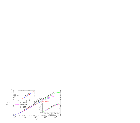
We have checked that the growth exponents for $(1+1)$-dimension are obtained correctly (both roughness and growth exponents $\alpha=1/2$ and $\beta=1/3$ respectively), and the (2+1)-dimensional results are given in Fig. 1, which are in good agreement with previous studies Parisi .

Figure 1: (color online). Main frame: Interface width $w_{L}(t)$ vs time $t$ of the KPZ equation in (2+1)-dimensions and for $\epsilon=10$, for different square lattice size $L$. The slope of the straight line yields the growth exponent $\beta=0.23\pm 0.01$. Upper-left inset: Saturation width $w_{L}(\infty)$ for systems of different size $L$. The slope of the solid-line fit yields the roughness exponent $\alpha=0.37\pm 0.01$. Lower-right inset: Rescaled $w_{L}$ vs rescaled $t$.

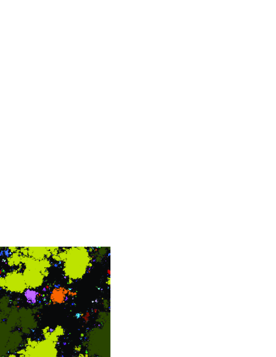
We now consider the saturated 2D-KPZ surface and set its mean height to be zero, and attribute the same sign to the points that have positive or negative heights. The same-sign regions (clusters) and their boundaries (loops) were identified by the Hoshen-Kopelman algorithm (Fig. 2).

Figure 2: (color online). The clusters with positive heights are shown for the 2D-KPZ interface with different colors. Negative-height regions are colored with black.

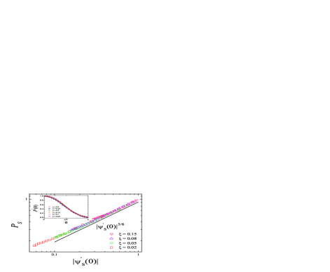
To investigate the scaling behavior of such loop ensembles in the 2D-KPZ interface, a set of scaling exponents associated with cluster and loop statistics were computed and checked, and are shown in Fig. 3 kondev ; Duplantier ; Cardy2 . The estimated exponents are in good agreement with the corresponding analytical results for SAWs in the scaling limit. The fractal dimension $D_{f}$ of contour lines obtained from the scaling relation between their length $l$ and radius of gyration $R$, i.e., $l\sim R^{D_{f}}$, is given by $D_{f}=1.33\pm 0.01$ which is in agreement with the one obtained by the box-counting method for the largest contour lines, $D_{f}=1.33\pm 0.02$. Comparing with the known fractal dimension of $SLE_{\kappa}$ curves $D_{f}=1+\kappa/8$ for $0\leq\kappa\leq 8$ , the contour lines may have conformal invariant scaling limit according to $SLE_{8/3}$.

The quantity that can confirm the SAW property of the contour lines is the restriction property. Suppose that $S$ is a hull in the upper-half plane $\mathbb{H}$ which is bounded away from the origin, and $\gamma$ is a simple SLE curve in $\mathbb{H}$ with $\kappa\leq 4$. Let $\Psi_{S}$ be a unique conformal map of $\mathbb{H}\backslash S$ onto $\mathbb{H}$, such that $\Psi_{S}(0)=0$, $\Psi_{S}(\infty)=\infty$ and $\Psi^{\prime}_{S}(\infty)=1$. The restriction property states that the distribution of curves conditioned not to hit $S$ is the same as the distribution of curves in the domain $\mathbb{H}\backslash S$. This happens only for $\kappa=8/3$, and it is shown that Schramm-Lawler the probability that a curve does not hit the hull $S$ is

$$P[\gamma\cap S=\emptyset]=|\Psi_{S}^{\prime}(0)|^{5/8}.$$ (2)

Figure 3: (color online). Cluster and loop statistics for the iso-height lines of 2D-KPZ surface and the EW surface are shown by the lower (different colors) and upper (green) graphs, respectively. The results for the EW have been shifted by a constant 1 in order to distinguish them from the 2D-KPZ results. (a) The average area $M$ vs the radius of gyration $R$. (b) The length of a loop $l$ vs the radius of gyration $R$. (c) Number of clusters of area between $M$ and $\lambda M$. (d) Number of loops of length between $l$ and $\lambda l$. (e) Number of loops of radius of gyration between $R$ and $\lambda R$. (f) Number of loops of area between $A$ and $\lambda A$. (g) The average area of loops $A$ vs the length $l$. In all figures $\lambda\simeq 1.05$. Solid lines show the corresponding analytical results for the SAWs (bottom) and O(2) model (top). The error bars are almost the same size as the symbols in the scaling regions, and have not been drawn. The change in the exponents relative to the SAWs in Figs. (c), (d), (e) and (f), is due to the roughness exponent kondev .

To examine this property directly for contour lines on the saturated 2D-KPZ surface, we proceed as follows. First, we identify all the cluster boundaries (contour lines): for each cluster an explorer walks on the zero height line as keeping the sites with positive height on the right. Then, we consider an arbitrarily placed straight line for each curve as a real axis and cut the portion of the curve above it. Using this procedure, we obtain an ensemble of contour lines in the half-plane which start at the origin and end on the real axis $x_{\infty}$. To obtain curves whose size is of order one, we rescale them by a factor of $N^{\nu}$, where $\nu=1/D_{f}$. Second, we consider the hull $S$ as a slit placed at various distances $\xi$ from the origin and various heights $h$, for which the map $\Psi_{S}$ is defined by, $\Psi_{S}(z)=\xi+\sqrt{(z-\xi)^{2}+h^{2}}$. After mapping the curves by $\varphi(z)=x_{\infty}z/(x_{\infty}-z)$ , we have checked Eq. (2) for the contour lines of the 2D-KPZ surface. As shown in Fig. 4, the result is consistent with Eq. (2) and implies the connection between the contour lines and both the SAWs and $SLE_{8/3}$.

Since the restriction property only holds for $SLE_{8/3}$ curves, we test the probability that an SLE curve passes to the left of a given point $z=\rho e^{i\theta}$, where $\theta$ is the angle between the point and the origin, and $\rho$ is the distance from the origin inside the upper half-plane. Given scale invariance, this probability is independent of $\rho$, and the theory of SLE predicts Left that

$$P^{\prime}_{\kappa}(\theta)=\frac{1}{2}+\frac{\Gamma\left(\frac{4}{\kappa}\right)}{\sqrt{\pi}\Gamma\left(\frac{8-\kappa}{2\kappa}\right)}{}_{2}F_{1}\left(\frac{1}{2},\frac{4}{\kappa};\frac{3}{2};-cot^{2}(\theta)\right)cot(\theta).$$ (3)

Here, ${}_{2}F_{1}$ is the hypergeometric function. The computed $P^{\prime}_{\kappa}(\theta)$ for the contour lines of the 2D-KPZ surface is also consistent with the analytical form with $\kappa=8/3\pm 1/10$ (Fig. 4).

Figure 4: (color online). Main frame: The probability that a contour line of 2D-KPZ surface in the upper half-plane does not hit the slits of height $0.05\leq h\leq 0.5$ placed at $\xi$ from origin on the real axis vs $|\Psi^{\prime}_{S}(0)|=|\xi|(\xi^{2}+h^{2})^{-1/2}$. The solid line is the corresponding analytical prediction for $SLE_{8/3}$ curves. The error bars are almost the same size as the symbols in the scaling region. Inset: The probability that such a contour line passes to the left of a point $z=\rho e^{i\theta}$, for $\rho=0.05,0.1,0.15,0.2,0.25$ and $0.3$. The solid line shows the prediction of SLE for $\kappa=8/3$.

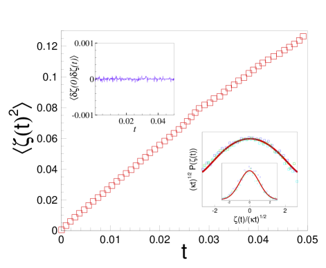
These results strongly suggest that the iso-height lines might be, in the scaling limit, conformally invariant, giving rise to the SLE curves with $\kappa=8/3$. To examine this suggestion directly, we can extract the Loewner driving function $\zeta$ of the curves using the successive conformal maps. We use the algorithm introduced by Bernard et al. bernard2 based on the approximation that driving function is a piecewise constant function. Each curve is parameterized by a dimensionless parameter $t$, to be distinguished from time in (1). The procedure is based on applying the map $G_{t,\zeta}=x_{\infty}\{\eta x_{\infty}(x_{\infty}-z)+[x_{\infty}^{4}(z-\eta)^{2}+4t(x_{\infty}-z)^{2}(x_{\infty}-\eta)^{2}]^{1/2}\}/\{x_{\infty}^{2}(x_{\infty}-z)+[x_{\infty}^{4}(z-\eta)^{2}+4t(x_{\infty}-z)^{2}(x_{\infty}-\eta)^{2}]^{1/2}\}$ on all the points $z$ of the curve approximated by a sequence of $\{z_{0}=0,z_{1},\cdot\cdot\cdot,z_{N}=x_{\infty}\}$ in the complex plane, where $\eta=\varphi^{-1}(\zeta)$ and again $\varphi(z)=x_{\infty}z/(x_{\infty}-z)$. At each step, by using the parameters $\eta_{0}=\varphi^{-1}(\zeta_{0})=[Rez_{1}x_{\infty}-(Rez_{1})^{2}-(Imz_{1})^{2}]/(x_{\infty}-Rez_{1})$ and $t_{1}=(Imz_{1})^{2}x_{\infty}^{4}/\{4[(Rez_{1}-x_{\infty})^{2}+(Imz_{1})^{2}]^{2}\}$, one point of the curve $z_{0}$ is swallowed and the resulting curve is rearranged by one element shorter. This operation yields a set containing $N$ numbers of $\zeta_{k}(t_{k})$ for each curve.

Figure 5: (color online). Statistics of the driving function $\zeta(t)$. Main frame: the linear behaviour of $\langle\zeta(t)^{2}\rangle$ with the slope $\kappa=8/3\pm 1/10$. Lower-right inset: The probability density of $\zeta(t)$ rescaled by its variance $\kappa$ at times $t=0.01,0.015,0.02$ which is Gaussian. Upper-left inset: The correlation function of the increments of the driving function $\delta\zeta(t)$. Kolmogorov-Smirnov (K-S) goodness of fit for normal distribution of the noise $\zeta(t)/\sqrt{\kappa t}$ for $\kappa=8/3$ and $0\leq t\leq 0.05$ yields $K-S=0.017$

.

The next step is analyzing the ensemble of the driving functions $\zeta(t)$ which can indicate, within the statistical errors, whether the curves are SLE or not. As shown in Fig. 5, the statistics of the ensemble of $\zeta(t)$ converges to a Gaussian process with variance $\langle\zeta^{2}(t)\rangle=\kappa t$ and $\kappa=2.6\pm 0.1$. This evidence certifies that the iso-height lines of 2D-KPZ interface in the saturation regime appear to be conformally invariant and are described by the $SLE_{8/3}$. The above results were obtained for $\epsilon=10$; however, the same analysis for growth surfaces with other values of $\epsilon$ (which were checked for $\epsilon=5$ and $25$) indicates no changes.

In the case of $\epsilon=0$, which corresponds to the EW model, comparing Fig. 6 and Fig. 2, indicates more ”porosity” in the clusters, which is indicative of changes in the cluster boundaries’ shape. As presented in Fig. 3, the cluster and loop statistics in this case are most consistent with those for the $O(2)$ model. These lead to the conclusion that if one assumes that the scaling limit of such contour lines exists, it should belong to the $SLE_{4}$ curves.

Figure 6: (color online). Positive height connected domains of 2D-KPZ interface without the non-linear term, corresponding to the EW model. Negative height regions are black.

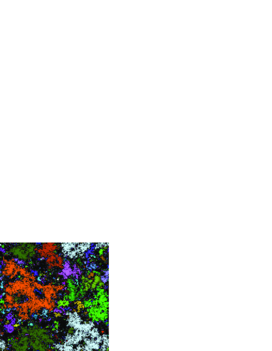
We also checked this directly as above and found that the driving function has Gaussian statistics with variance $\kappa=3.7\pm 0.2$.

The height clusters and their boundary statistics, in the manner presented here, can be applied to model the experimental grown surfaces by using an ensemble of the grown samples in the saturated regime. Since this analysis is far more accurate, it may be also used to investigate wether a model belongs to a universality class or not. For example, the small difference between the cluster analysis of the BD model WO3 ; krug1 ; krug2 and KPZ equation in two dimensions can be revealed.

We wish to thank J. Cardy for useful hints on this work. We also thank S. Moghimi-Araghi, M. A. Rajabpour and M. Sahimi for useful discussions.

References

- (1) D. Bernard, et al., Nature Phys. 2, 124 (2006).
- (2) D. Bernard, et al., Phys. Rev. Lett. 98, 024501 (2007).
- (3) C. Amoruso, et al., Phys. Rev. Lett. 97, 267202 (2006); D. Bernard, et.al, Phys. Rev. B 76, 020403(R) (2007).
- (4) J. P. Keating, et al., Phys. Rev. Lett. 97, 034101 (2006); E. Bogomolny, et al., [nlin/0609017].
- (5) A. A. Saberi, et.al, Phys. Rev. Lett, 100, 044504 (2008).
- (6) O. Schramm, Israel. J. Math. 128, 221 (2000).
- (7) J. Cardy, Ann. Physics 318, 81 (2005); M. Bauer and D. Bernard, Phys. Rep. 432, 115 (2006); I. A. Gruzberg, J. Phys. A: Math. Gen. 39, 12601 (2006); H. C. Fogedby, [cond-math/0706.1177].
- (8) O. Schramm and S. Sheffield, [Math.PR/0605337] (2006).
- (9) GF. Lawler, et al., J. Amer. Math. Soc. 16, 917 (2003).
- (10) T. Kennedy, Phys. Rev. Lett. 88, 130601 (2002).
- (11) G. Lawler, et al., arXiv:math/0204277.
- (12) M. Kardar, G. Parisi and Y.-C. Zhang, Phys. Rev. Lett. 56, 889-892 (1986).
- (13) A. L. Barab si and H. E. Stanley, Fractal Concepts in Surface Growth (Cambridge University Press, Cambridge, 1995).
- (14) M. S. Miguel and R. Toral, Instabilities and Nonequilibrium Structures, (Kluver Academic Publishers, vol. VI, p. 35, 2000).
- (15) C. Dasgupta, et al., Phys. Rev. E 55, 2235 (1997); C. Dasgupta, et al., Phys. Rev. E 54, R4552 (1996).
- (16) J. G. Amar, F. Family, Phys. Rev. A 41, 6, 3399 (1990); E. Marinari, et al., J. Phys. A: Math. Gen. 33, 8181 (2000).
- (17) J. Kondev, C. L. Henley, Phys. Rev. Lett, 74, 23, 4580 (1995).
- (18) B. Duplantier, Phys. Rev. Lett, 64, 4, 493 (1990).
- (19) J. Cardy, Phys. Rev. Lett, 72, 1580-1583 (1994).
- (20) O. Schramm, Electron. Commun. Probab. 6, 115 (2001).
- (21) P. Meakin and J. Krug, Europhys. Lett. 11, 7-12 (1990).
- (22) P. Meakin and J. Krug, Phys. Rev. A 46, 3390-3399 (1992).