Zeeman-Tomography of the solar photosphere

Abstract

Aims. The thermodynamic and magnetic field structure of the solar photosphere is analyzed by means of a novel 3-dimensional spectropolarimetric inversion and reconstruction technique.

Methods. On the basis of high-resolution, mixed-polarity magnetoconvection simulations, we used an artificial neural network (ANN) model to approximate the nonlinear inverse mapping between synthesized Stokes spectra and the underlying stratification of atmospheric parameters like temperature, line-of-sight (LOS) velocity and LOS magnetic field. This approach not only allows us to incorporate more reliable physics into the inversion process, it also enables the inversion on an absolute geometrical height scale, which allows the subsequent combination of individual line-of-sight stratifications to obtain a complete 3-dimensional reconstruction (tomography) of the observed area.

Results. The magnetoconvection simulation data, as well as the ANN inversion, have been properly processed to be applicable to spectropolarimetric observations from the Hinode satellite. For the first time, we show 3-dimensional tomographic reconstructions (temperature, LOS velocity, and LOS magnetic field) of a quiet sun region observed by Hinode. The reconstructed area covers a field of approximately $12\;000\times 12\;000$ km and a height range of $510$ km in the photosphere. An enormous variety of small and large scale structures can be identified in the 3-D reconstructions. The low-flux region ($B_{mag}=20G$) we analyzed exhibits a number of tube-like magnetic structures with field strengths of several hundred Gauss. Most of these structures rapidly loose their strength with height and only a few larger structures can retain a higher field strength to the upper layers of the photosphere.

1 Introduction

There has been a growing interest in the (small-scale) magnetic field from low-flux regions (i.e. internetwork) over the recent years (e.g. Lites 2002; Lites & Socas-Navarro 2004; Socas-Navarro et al. 2004; Khomenko et al. 2005; Domínguez Cerdeña et al. 2006; López Ariste et al. 2007), not least because these regions make up most of the solar surface and may therefore carry most of the unsigned magnetic flux and magnetic energy (Sánchez Almeida 2004). Spectropolarimetric observations and their analysis are extremely challenging in these low-flux regions because of the weakness of the polarimetric signals and because of the complex arrangement and small filling factor of the underlying magnetic field. Despite these complexities, the analysis of spectropolarimetric observations in terms of a Stokes profile inversion may still be the most promising way to reveal the magnetic properties of these low-flux regions. A number of different inversions have recently been applied to spectropolarimetric observations from internetwork regions (e.g. Sánchez Almeida & Lites 2000; Socas-Navarro & Sánchez Almeida 2002; Domínguez Cerdeña et al. 2006; Orozco Suárez et al. 2007) and could retrieved one-dimensional (depth independent) estimates of the magnetic field strength for each line-of-sight (LOS). But, as model assumptions and constraints are inevitable, the question arises to what extent these assumptions are physically meaningful and how inversions can yield reliable results. In this context, note the potential degeneracy that can be caused by the subtle interplay between thermodynamics and magnetic fields (Martínez González et al. 2006).

To implement more physical realism and more reliable contraints into the inversion process we have incorporated the most recent magnetohydrodynamic (MHD) simulations (Vögler et al. 2005) into an artificial neural network (ANN) inversion (Carroll & Staude 2001). This inversion which takes into account the full dynamical situation present in the MHD data, allows us to extract the depth stratification of the temperature, LOS velocity, and the LOS magnetic field. Moreover, this approach facilitates the inversion on an absolute height scale, and thus the 3-dimensional reconstruction (tomography) of the entire field-of-view (FOV).

2 Basic strategy

Our approach is based on the assumption that MHD simulations have reached a degree of realism that allows them to provide a meaningful and quantitative representation of magnetoconvective processes in the solar photosphere. If this assumption is approximately true, MHD simulations can be used to generate a large and statistically significant sample of possible magnetoconvective scenarios such that a machine learning algorithm (Bishop 1995) can extract the underlying generator (function), which describes the relationship between the Stokes spectra and the atmospheric parameters.

3 MHD-Simulations, spectral synthesis, image and data degradation

To provide a large and quasi-realistic sample of possible magnetic and thermodynamic scenarios for the training process of the ANNs, we have used recent high-resolution, non-grey, mixed-polarity MHD simulations (Vögler et al. 2005), which comprises three snapshots of different magnetic regimes. One snapshot has an average unsigned magnetic field strength of $\langle B\rangle$ = 22 G, and represents a low-flux region typical for the internetwork; a second one covers a medium range with an average unsigned field strength of $\langle B\rangle$ = 50 G; and a third one represents a strong-flux scenario with $\langle B\rangle$ = 144 G, comparable to an active plage region. Each simulation snapshot covers a computational domain of 6000 $\times$ 6000 $\times$ 1400 km³, which is discretized by 576 $\times$ 576 $\times$ 100 grid points. Based on the depth stratification of the individual MHD snapshots we have carried out the synthesis of the Stokes spectra for each LOS (assuming disc center observations) for the two iron lines Fe i 6301.5 Å and Fe i 6302.5 Å .

To make synthetic profile images comparable to observations from the Solar Optical Telecope (SOT) and the spectropolarimeter (SP) of Hinode (Lites et al. 2001; Shimizu 2004), we followed the same procedure as described by Orozco Suárez et al. (2007). We first degraded the synthetic profile images by an appropriate modulation transfer function (MTF) which also accounts for the effect of the finite CCD pixel size. We then resampled (rebinned) the profile images according to the CCD pixel size of 0.16″$\times$ 0.16″and finally convolved the individual profiles with a Gaussian function of 30 mÅ FWHM to account for the limited resolving power of the spectrograph.

To assure the agreement between the individual Stokes spectra and the underlying atmospheric parameters on a spatial scale of 0.16″$\times$ 0.16″, we applied to the MHD snapshots, which contain the atmospheric data (temperature, velocity and magnetic field) the same resampling and averaging (rebinning) procedure as for the spectral images. Thus, each of the 100 depth level in the original MHD snapshots has been resampled to obtain a mean depth stratification (for each parameter) in each resampled pixel. Note, that the original sampling of the high-resolution MHD simulation corresponds to a spatial scale of 0.014″$\times$ 0.014″such that the resampled profile images and data layers comprises more than 11 $\times$ 11 pixel of the original MHD snapshot. This smearing can already lead to a significant reduction in the peak values of the magnetic field strength (up to 25% in our case).

4 Artificial neural network inversion and tomography

Our inversion is based on multi-layer perceptrons (MLPs), a popular type of artificial neural networks (Bishop 1995) that have already been successfully applied in the field of Stokes profile inversions (Carroll & Staude 2001; Socas-Navarro 2005). Based on the data provided by the MHD simulations and the synthetic Stokes profiles, we have trained three different MLPs to approximate the nonlinear mapping between the Stokes profiles of the two iron lines and the underlying stratification of the temperature, the LOS velocity, and the LOS component of magnetic field vector. From each of the three available MHD snapshots we extracted a set of 5000 Stokes spectra together with the underlying depth stratification of the atmospheric data. The 5000 different positions were obtained by randomly placing a sliding window (11 $\times 11$ pixels) on the original snapshots. This procedure allowed us to compile a dataset of 15 000 depth stratifications (for all 3 parameters) together with their corresponding (degraded) synthetic Stokes spectra. To each spectra we added Gaussian noise of a level of 10^-3, which is comparable to the expected noise level of Hinode/SP (Lites et al. 2001). Since we are, in particular, interested in analyzing Stokes profiles from low-flux regions we concentrate on Stokes $I$ and Stokes $V$ profiles only and refrain from analyzing the weak linear polarization signal in this work.

Since the intrinsic dimensionality of the Stokes profiles is usually much less than the typical wavelength sampling (Asensio Ramos et al. 2007), we have applied a principal component analysis (PCA) (Rees et al. 2000) to our database of synthetic Stokes profiles. The PCA allows us to describe efficiently each of the two iron Stokes $I$ profiles by using the first 10 eigenvectors (principal components) only. This provides a RMS reconstruction error as low as 10^-4 for the entire database. Due to the higher relative noise level we used only 5 principal components for each of the Stokes $V$ profiles, which still allows for a RMS reconstruction error smaller than 5 $\times$ 10^-4, and thus well below the assumed noise level.

Even after the resampling and averaging of the atmospheric parameters, the individual stratifications in each pixel still exhibit a complex and sometimes irregular variation along the LOS. To efficiently but also accurately describe the individual depth stratifications we have to choose an appropriate and flexible description. For this reason, we took advantage of the exhaustive statistics provided by the MHD simulations (15 000 stratifications) to apply a principal component analysis (PCA) to the depth stratification of the atmospheric parameters. We have decomposed the stratifications of the temperature, the LOS velocity and the LOS magnetic field for the upper 510 km, which comprises 37 grid point in the original MHD snapshots. After calculating the PCA for the entire database each atmospheric stratification could be sufficiently described by using only the five principal components (eigenvectors). The appropriateness of this parameterization can be evaluated by reproducing the 37 original grid points for each LOS from the five projection coefficients. The mean reproduction error per grid point for all available 15 000 depth stratifications are 1.05 Gauss for the LOS component of the magnetic field vector, 59.43 m/s for the LOS velocity, and 37.84 K for the temperature.

Three separate MLPs are used to retrieve the temperature, velocity, and magnetic field information along the LOS. One MLP is trained to approximate the mapping between the two PCA decomposed Stokes $I$ profiles of the iron lines and the PCA decomposed temperature stratification; another one for the mapping between the decomposed Stokes $I$ profiles and the decomposed velocity stratification; and a third one for the mapping between the two decomposed Stokes $V$ profiles and the decomposed magnetic field stratification. The training process of the MLPs follows that described in detail by Carroll et al. (2001); Carroll & Staude (2001). Since the original atmospheric stratifications in the MHD simulations are given on an absolute geometrical height scale, the MLPs describe the inverse mapping on the same absolute scale that comprises a height range of 510 km and corresponds to a mean logarithmic optical depth range between 0.6 and -4.0. This fact facilitates the subsequent combination of the individual results from the LOS inversion to yield a complete 3-dimensional reconstruction of the observed area.

The trained MLPs have been tested by applying unknown synthetic Stokes $I$ and $V$ profiles from a MHD snapshot ($\langle B\rangle$ = 22 G) that were not part of the training database. The MHD test case comprises 50 $\times$ 50 $\times$ 37 (92 500) grid points for each of the three atmospheric parameter. Before the synthetic Stokes spectra of this test case were presented to the MLPs the profiles went through the same degradation and decomposition process as the training data and were additionally corrupted by noise of 10^-3. The individual MLPs then completely reconstructed the atmospheric structure of the MHD test case from the Stokes $I$ and $V$ spectra of the two iron lines. The mean absolute error per grid point (with respect to the MHD test snapshot) for the test case was 73.51 K for the temperature, 195.08 m/s for the velocity, and only 5.79 G for the LOS magnetic field component. A detailed analysis of the individual MLPs and the presentation of the impressive results will be given in a forthcoming paper (Carroll 2008).

5 The real case, tomography of a quiet Sun region

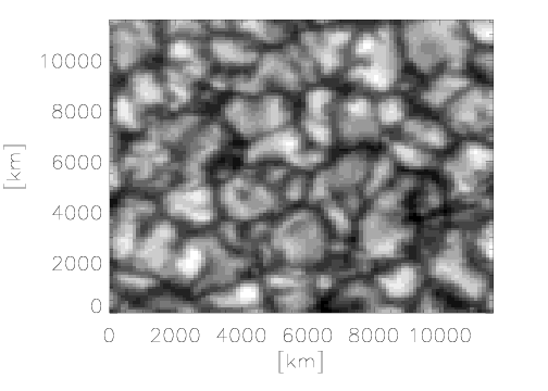
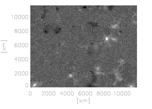
The observation we used were taken on March 10, 2007 with the spectropolarimeter (SP) aboard Hinode. The scan comprises a quiet sun region at disc center and covers a FOV of 302” $\times$ 162”. The SP recorded the Stokes spectra of the iron line pair at FeI 6301 Å with a wavelength sampling of 2.15 pm. The data have been corrected for dark current, flat field, and instrumental effects as described by Lites (2007). We conducted a wavelength calibration and continuum normalization according to the procedure described by (Jurčák et al. 2007). As explained in the preceding section we designed the preparation of the MHD data and spectra as well as the neural network training to match Hinode/SP observations. Thus, we could directly decompose the measured Stokes profiles and apply them to the individual MLPs. Note that due to the processing of the MHD data (resampling) the ANN inversion operates on a spatial scale that corresponds to the CCD pixel size of 0.16” $\times$ 0.16” and therefore facilitates a one-component inversion on that scale. The inversions and 3-dimensional reconstructions were made for the entire FOV but for the sake of clarity and a better illustration of the results we confine ourselves to a subregions that covers an area of 100 $\times$ 100 pixel (16” $\times$ 16” $\approx$ 11 600 $\times$ 11 600 km). The continuum and the magnetic flux density estimation (as retrieved from the measured Stokes $V$ profiles) are shown in Fig.1. From the magnetic flux density estimation we deduce a mean unsigned flux density $B_{mag}$ of approximately 20 G for the subregion.

Figure 1: Continuum intensity (left) and magnetic flux density (right) for the analyzed quiet-sun region. The small circle on the lower right in the flux density figure indicates a strong flux structure which will be shown in greater detail in the following tomographic reconstruction

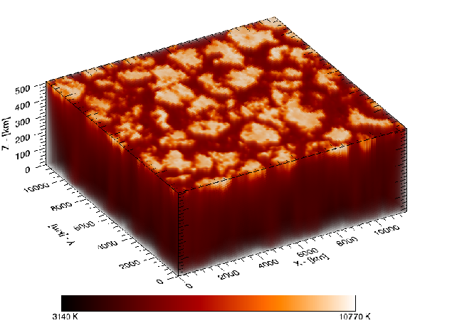
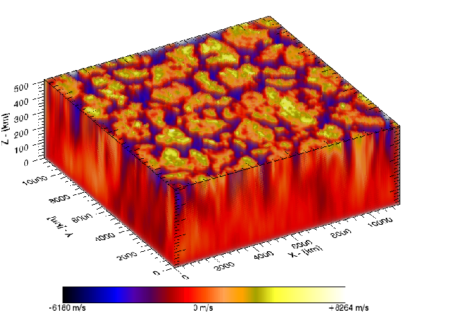
The results of the temperature and the LOS velocity tomography are shown in Fig.2 and Fig.3. For the purpose of showing the rich and detailed structure of the 3-dimensional reconstructions, the data volumes are shown in a bottom view (upside down) such that the deepest layers of the photosphere ($<$log$(\tau)$$>$ $\approx$ 0.6) are on top.

Figure 2: Tomographic reconstruction of the temperature for the analyzed photospheric region. For the purpose of a better visualization, the reconstructed 3-dimensional surface volume is shown in bottom view. Note how the bright (hot) and the dark (cool) areas in the deep layers (here on top) nicely reproduce the granulation pattern (Fig.1).

Figure 3: 3-Dimensional reconstruction of the LOS velocity. As in Fig.2 the reconstruction shows the deepest layer on top. Yellow and orange colors indicate strong upflows (here in the downward direction), and blue and dark colors indicate downflows (here upward direction). Note the onset of strong downflows (blue) in the mid-photosphere

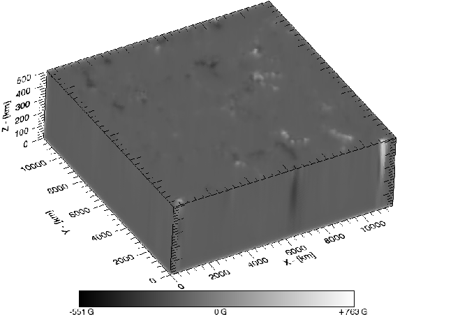
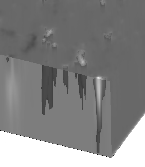
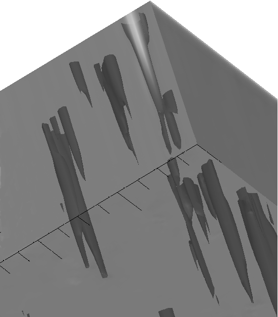
The tomography of the LOS magnetic field for the subregion is shown in Fig.4. This reconstruction is also in a bottom up view to give a better illustration of the many details in the lower atmosphere. The bipolar features of the flux density estimation of Fig.1 are well reproduced, but in much greater detail and, moreover, many fine scale structures are visible at the bottom layer at $<$log$(\tau)$$>$ $\approx$ 0.6. The whole 3-dimensional reconstruction comprises 370 000 (100 $\times$ 100 $\times$ 37) grid points. In the front X-Z plane of Fig.4, we see that our tomography reveals the slice view of three magnetic structures. A close-up view of one of these magnetic structures is shown in Fig.5 and Fig.6. The position of this structure is marked by the encircled region in the flux density image (Fig.1) and in the 3-D reconstruction (Fig.4). The side wall (X-Z plane) of Fig.5 as well as the bottom plane (X-Y plane) in Fig.6, are made transparent to allow a view into the inner part of the reconstructed data volume. Isosurfaces of +175 G are made visible, revealing the existence of many tube-like magnetic structures. One can see that the depicted strong magnetic feature in Fig.5 and Fig.6 exhibits not only a tube-like character but also an internal structure with vertical and lateral gradients (increased whitening towards the inner). This internal structuring is also characterized by the increased narrowing of the flux structures toward the upper atmosphere (again note, the bottom up view of the representation). It is also conspicuous that many of the isosurfaces do not reach the upper layers of the atmosphere, indicating the rapid decrease of magnetic field strength with height. This fact will be highlighted in our upcomming paper (Carroll 2008) in which we present the first 3-dimensional empirical probability density functions (pdfs) for the magnetic field strength. These pdfs reveal the characteristic height dependent changes (shift of mean and varaiance) of the magnetic field strength. In this context, it is also interesting to note that the mean unsigned flux at the bottom layer in the reconstructed volume decreases from 15.88 G to 4.24 G at the top layer (510 km above). This also indicates that much of the magnetic flux does not reach the upper photosphere in the form of magnetically dense flux structures. The peak field strength of 763 G in the analyzed 3-dimensional region is encountered on the footpoint of the depicted magnetic structure and is marked by the circle in Fig.5. Note, the maximum value in the flux density estimation (Fig.1) only yields 297 G for this structure.

Figure 4: The 3-dimensional reconstruction of the LOS magnetic field. As in Fig.2 & Fig.3 the reconstruction is shown in a bottom up view. Bright and dark colors represent the different magnetic polarities. The marked region which comprises the magnetic structure encircled in Fig.1 provides a cross-section view of this structure.

Figure 5: A close up view of the magnetic structure, marked in Fig.4, shown with transparent X-Z plane and iso-surfaces of 175 G. It shows a cross-section through the tube-like magnetic structure. The highest field strength of 763 G is reached within the encircled region.

Figure 6: Another close up view of the same structure, but from a different viewing angle. The data volume is rotated around the X and Y axes (lifted) to allow a view through the transparent bottom plane of the box. This view corresponds to an oblique view from the top of the atmosphere.

6 Discussion and conclusion

We have presented an inversion approach based on artificial neural networks that incorporates the knowledge from high-resolution, mixed-polarity magnetoconvection simulations. This approach does not only allow the accurate determination of the depth stratification of various atmospheric parameters, it also facilitates the complete 3-dimensional reconstruction of the analyzed atmosphere. The tomography retrieves the information from a surface layer of 510 km in the photosphere, which covers a mean logarithmic optical depth range from 0.6 to -4.0. The presented inversion approach allows a unique 3-dimensional investigation of individual photospheric structures. Based on Hinode/SOT observations of a quiet sun region, this work has demonstrated the feasibility of a tomographic reconstruction for the temperature, LOS velocity, and magnetic field. Nevertheless, it is important to emphasize that this approach is based on the premise that MHD simulations have reached a sufficient degree of realism and that the simulation snapshots used in this work provide a statistically relevant sample of possible physical scenarios encountered in the solar photosphere. If these conditions are met, the presented ANN approach and tomography provides a powerful and exciting new diagnostic for the magnetic field of the solar photosphere.