Frequency Light Shifts Caused by the Effects of Quantization of Atomic Motion in an Optical Lattice

Abstract

Frequency light shifts resulting from the localization effects and effects of the quantization of translational atomic motion in an optical lattice is studied for a forbidden optical transition $J$=0$\to$$J$=0. In the Lamb-Dicke regime this shift is proportional to the square root from the lattice field intensity. With allowance made for magneto-dipole and quadrupole transitions, the shift does not vanish at the magic wavelength, at which the linear in intensity shift is absent. Preliminary estimates show that this shift can have a principal significance for the lattice-based atomic clocks with accuracy of order of 10^-16-10^-18. Apart from this, we find that the numerical value of the magic frequency depends on the concrete configuration of the lattice field and it can vary within the limits 1-100 MHz (depending on element) as one passes from one field configuration to another. Thus, theoretical and experimental investigations of contributions originated from magneto-dipole and quadrupole transitions are of principal self-dependent interest.

The last few years were marked by a principal ideological Katori1 and experimental Katori2 ; Ye1 ; Bar06 ; Lemonde1 ; Ye2 breakthrough in the field of fundamental laser metrology based on a possibility to work with strongly forbidden optical transitions, using large number of neutral atoms confined to an optical lattice at the magic wavelength. This great advance expressed itself in a transition to spectral structures with Hertz Bar06 ; Ye2 and potentially sub-Hertz widths, that approaches a prospect of the creation of atomic optical frequency standards with unprecedented fractional frequency uncertainty and accuracy at a level 10^-17-10^-18.

However the achievement of such extraordinary metrological characteristics in real frequency standards is a challenging goal. On the way to this goal it will be necessary to determine sources and values of systematic errors. Therefore now there comes a period, when frequency shifts of various origin should be thoroughly investigated. For example, the second-order (in intensity) light shift due to the atomic hyperpolarizability has been studied experimentally Lemonde1 ; Bar08 and theoretically TY06_2 .

In the present paper, taking into account contributions due to magneto-dipole and quadrupole transitions, we investigate a previously unknown frequency light shift caused by the quantization of atomic translational motion in an optical lattice for a forbidden optical transition $J_{g}$=0$\to$$J_{e}$=0 (for instance, ${}^{1}S_{0}$$\to$${}^{3}P_{0}$ in alkaline-earth-like atoms). This shift is proportional to the square root (in the Lamb-Dicke regime) from the lattice field intensity, and it does not vanish at the magic wavelength $\lambda_{m}$, at which the first-order (in intensity) light shift cancels. Preliminary estimates show that this unavoidable shift has a principal significance for the definition of metrological characteristics of lattice-based atomic clocks.

Note, the influence of the electric quadrupole ($E2$) and magnetic dipole ($M1$) effects on the clock levels in Sr atoms was first discussed in Katori1 . The calculations have demonstrated that the $E2$ and $M1$ dynamic polarizabilities at the magic wavelength is of order $10^{-7}$ of the electric dipole ($E1$) polarizability. However, the calculations in Katori1 referred to the usual plane-wave approach which did not account for the specific inhomogeneous distribution in space of electric and magnetic field components of the optical lattice. The effects of inhomogeneous field distribution of a standing wave are considered in the present paper in detail.

Consider an atom confined to an optical lattice, which is induced by a one-dimensional elliptically polarized standing wave (with the frequency $\omega$). The electric field vector has the form:

$${\bf E}({\bf r},t)=E_{0}{\bf e}\cos({\bf k}\cdot{\bf r})\,e^{-i\omega t}+c.c.\,,$$ (1)

where $E_{0}$ is the scalar amplitude; ${\bf k}$ is the wavevector ($k$=$|{\bf k}|$=$\omega$/$c$); ${\bf e}$ is the complex unit polarization vector $({\bf e}\cdot{\bf e}^{*})$=1. The condition $({\bf e}\cdot{\bf k})$=0 is satisfied due to the transversality of electromagnetic field.

First we consider the frequency shift of a transition $J_{g}$=0$\to$$J_{e}$=0 in a potential induced only by the contributions of electro-dipole transitions $J_{j}$=0$\to$$J$=1 ($j$=$g$,$e$). For the standing-wave field (1) the light shift (potential) of a $j$-th level is spatially modulated and it has the following form:

$$U^{E}_{j}({\bf r})=-{\cal W}_{j}\cos^{2}(kz)\,;\quad{\cal W}_{j}>0\quad(j=g,e)\,.$$ (2)

Here, for convenience, we direct the $z$ axis along the wavevector ${\bf k}$. The potential amplitude ${\cal W}_{j}$ depends on the frequency $\omega$ and it is proportional to $|E_{0}|^{2}$.

Then we quantize the translational motion of atoms. To do this we will assume the Lamb-Dicke regime, when atoms are localized in the field antinodes $kz$=$l$$\pi$ ($l$=0,$\pm 1$,$\pm 2$…) on the size much less than the wavelength. In this case we can describe the atomic motion in the harmonic approximation. For the sake of definiteness, we will work near the point $z$=0. At the condition $|kz|$$\ll$1 we can use the approximation $\cos^{2}(kz)$$\approx$1$-$$k^{2}$$z^{2}$, which allows us to write the shift (2) as the harmonic oscillator potential:

$$U^{E}_{j}({\bf r})\approx-{\cal W}_{j}+\frac{M(2\pi\Omega_{j})^{2}z^{2}}{2}\,;\qquad(j=g,e)\,,$$ (3)

where $M$ is the atomic mass, and the oscillator frequency $\Omega_{j}$ for $j$-th level has the form:

$$\Omega_{j}=\frac{1}{2\pi}\sqrt{\frac{2{\cal W}_{j}\,k^{2}}{M}}\,;\qquad(j=g,e)\,.$$ (4)

The following relationships are obvious:

$${\cal W}_{j}\propto I\,,\quad\Omega_{j}\propto\sqrt{I}\,,$$ (5)

where $I$=$c$$|E_{0}|^{2}$/2$\pi$ is the field intensity in the lattice antinode.

Using for the potential (3) the standard theory of harmonic oscillator, we write the energies of the upper and lower levels with consideration for the vibrational structure:

$${\cal E}_{j}(n)={\cal E}_{j}^{(0)}-{\cal W}_{j}+h\Omega_{j}(n+1/2)\,,\quad(j=g,e),$$ (6)

where $h$=2$\pi$$\hbar$; ${\cal E}_{j}^{(0)}$ is the energy of unperturbed $j$-th state in a free space; $n$=0,1,2,… is the vibrational quantum number (see in Fig.1).

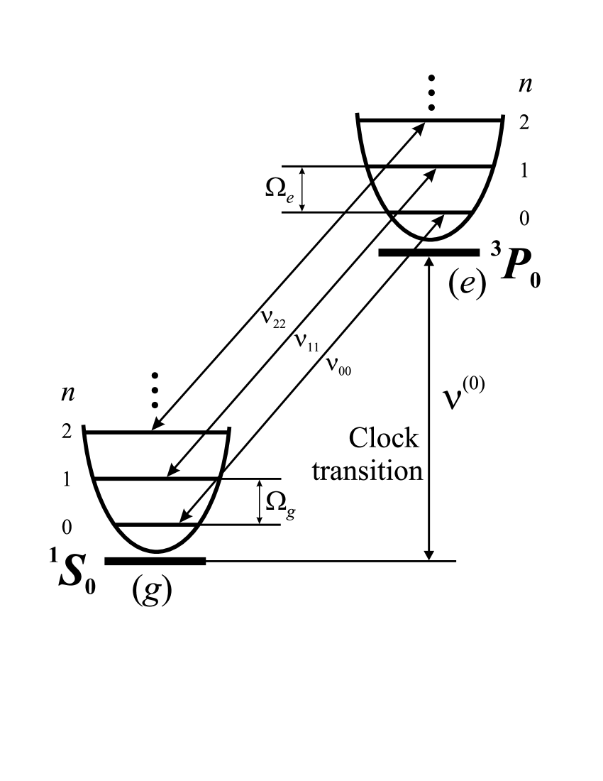
Figure 1: An illustration of optical transitions between vibrational levels for atoms confined to an optical lattice.

Consider the optical frequency of transition between vibrational levels with the same quantum numbers $n$:

$$\nu_{nn}=\frac{{\cal E}_{e}(n)-{\cal E}_{g}(n)}{h}=$$ (7)

$$\nu^{(0)}-({\cal W}_{e}-{\cal W}_{g})/h+(\Omega_{e}-\Omega_{g})(n+1/2)\,,$$

where $\nu^{{(0)}}$=(${\cal E}_{e}^{(0)}$$-$${\cal E}_{g}^{(0)}$)/$h$ is the frequency of unperturbed $J_{g}$=0$\to$$J_{e}$=0 transition. Taking into account the relationships (5), the frequency shift can be written as:

$$\Delta\nu_{nn}\equiv\nu_{nn}-\nu^{{(0)}}=\alpha(\omega)I+(n+1/2)\beta(\omega)\sqrt{I}\,,$$ (8)

where the coefficients $\alpha(\omega)$ and $\beta(\omega)$ are individual characteristics of chosen element. They are defined as follows:

$$\alpha(\omega)I=-({\cal W}_{e}-{\cal W}_{g})/h\,;\;\;\beta(\omega)\sqrt{I}=\Omega_{e}-\Omega_{g}\,.$$ (9)

Thus, despite of the fact that we consider the potential (2), which is proportional to $I$, the effects of the quantization of atomic motion lead (in the Lamb-Dicke regime) to the appearance of the additional square root dependence ($\propto$$\sqrt{I}$) for the frequency shift (8). Note that beyond the Lamb-Dicke regime the intensity dependence of the frequency shift is more complicated due to the anharmonicity.

In the case of potential (2), which is induced by electro-dipole transitions only, at the magic frequency $\omega_{m}$=2$\pi$$c$/$\lambda_{m}$ we have simultaneously $\alpha(\omega_{m})$=0 and $\beta(\omega_{m})$=0, because ${\cal W}_{e}(\omega_{m})$=${\cal W}_{g}(\omega_{m})$. However, if we take into account contributions due to magneto-dipole and quadrupole transitions, it will not be so, i.e. $\beta(\omega_{m})$$\neq$0, that can have a principal importance for metrological characteristics. Let us prove this.

For the standing-wave field (1) the magnetic field vector ${\bf B}$ has the form:

$${\bf B}({\bf r},t)=B_{0}{\bf e}_{B}\sin({\bf k}\cdot{\bf r})\,e^{-i\omega t}+c.c.\,,$$ (10)

where $B_{0}$=$iE_{0}$ is the scalar amplitude of the magnetic field, and ${\bf e}_{B}$=$[{\bf k}$$\times$${\bf e}]$/$k$ is the unit polarization vector of the magnetic field. As a result, the contribution to the potential of $j$-th level ($\propto$$|{\bf B}|^{2}$) due to magneto-dipole transitions $J_{j}$=0$\to$$J$=1 has the spatial dependence different from the potential (2):

$$U^{B}_{j}({\bf r})={\cal B}_{j}\sin^{2}(kz)\,;\qquad(j=g,e)\,,$$ (11)

where the potential amplitude ${\cal B}_{j}$ is proportional to the intensity $I$, but the frequency dependence (on $\omega$) of ${\cal B}_{j}$ differs from ${\cal W}_{j}$. It can be easily shown that the contribution due to quadrupole transitions $J_{j}$=0$\to$$J$=2 has the same spatial dependence (for 1D standing wave):

$$U^{Q}_{j}({\bf r})={\cal Q}_{j}\sin^{2}(kz)\,;\qquad(j=g,e)\,.$$ (12)

Hence, for $j$-th level the total potential proportional to the intensity $I$ has the form:

$$U_{j}({\bf r})=U^{E}_{j}({\bf r})+U^{B}_{j}({\bf r})+U^{Q}_{j}({\bf r})=$$ (13)

$$-{\cal W}_{j}\cos^{2}(kz)+\{{\cal B}_{j}+{\cal Q}_{j}\}\sin^{2}(kz);\quad(j=g,e).$$

As is seen, the spatial dependencies of potentials $U_{g}({\bf r})$ and $U_{e}({\bf r})$ for the lower and upper levels of the forbidden $J_{g}$=0$\to$$J_{e}$=0 transition are different due to the contributions induced by magneto-dipole and quadrupole transitions, i.e. $U_{g}({\bf r})$$/$$U_{e}({\bf r})$$\neq$$\,const$. As a consequence, strictly speaking, the condition $U_{e}({\bf r})$=$U_{g}({\bf r})$ does not hold for any frequency. Hence, the ideal notion of the magic frequency $\omega_{m}$ does exist only for a single running wave, for which, however, the confining optical lattice potential is absent (spatially uniform light shift) and therefore this case is not important for lattice-based atomic clock. However, since the contribution due to electro-dipole transitions dominates, the other contributions can be considered as very small perturbation, which, nevertheless, can influence the metrological characteristics of frequency standards.

Expanding the expression (13) in $(kz)$ powers and using the harmonic approximation (i.e. $\cos^{2}(kz)$$\approx$1$-$$k^{2}$$z^{2}$ and $\sin^{2}(kz)$$\approx$$k^{2}$$z^{2}$), we obtain the expression for the potential analogous to (3):

$$U_{j}({\bf r})\approx-{\cal W}_{j}+\frac{M(2\pi\widetilde{\Omega}_{j})^{2}z^{2}}{2}\,;\qquad(j=g,e)\,,$$ (14)

from which all the following formulae (5)-(9) are deduced. However instead of $\Omega_{j}$ (see eq.(4)) now we have to use the other expression for the vibrational frequency $\widetilde{\Omega}_{j}$:

$$\widetilde{\Omega}_{j}=\frac{1}{2\pi}\sqrt{\frac{2\left\{{\cal W}_{j}+{\cal B}_{j}+{\cal Q}_{j}\right\}k^{2}}{M}};\quad(j=g,e).$$ (15)

From the equations (14) and (15) it follows that for 1D standing wave the magneto-dipole and quadrupole transitions affect only the coefficient $\beta(\omega)$ in the formula for the shifts (8), while the coefficient $\alpha(\omega)$ is governed by the electro-dipole transitions solely as before.

The magic frequency of lattice field $\omega_{m}$ can now be determined from the condition of cancelation of the linear (with respect to the intensity $I$) shift in (8) (i.e. $\alpha(\omega_{m})$=0). In this case we find that ${\cal W}_{e}(\omega_{m})$=${\cal W}_{g}(\omega_{m})$=${\cal W}$. Then the remaining shift ($\propto$$\sqrt{I}$) in eq.(8) differs from zero:

$$\Delta\nu_{nn}=(n+1/2)\beta(\omega_{m})\sqrt{I}\neq 0\,.$$ (16)

Expanding the expression (15) in small parameter $|$$({\cal B}_{j}$+${\cal Q}_{j})$/${\cal W}$$|$$\ll$1 and leaving only the first-order term, we obtain:

$$\beta(\omega_{m})\sqrt{I}=(\widetilde{\Omega}_{e}-\widetilde{\Omega}_{g})\approx{\Omega}^{(0)}\eta\,.$$ (17)

Here the frequency $\Omega^{(0)}$ is equal to:

$${\Omega}^{(0)}=\frac{1}{2\pi}\sqrt{\frac{2{\cal W}k^{2}}{M}}\,,$$ (18)

and its value coincides with the vibrational frequency, which is practically the same (at $\omega_{m}$) for the upper and lower levels of the clock transition $J_{g}$=0$\to$$J_{e}$=0. The dimensionless small coefficient $\eta$ in (17) does not depend on the intensity $I$ and polarization ${\bf e}$, and it is defined as:

$$\eta=\eta_{B}+\eta_{Q}\,;$$ (19)

$$\eta_{B}=\frac{{\cal B}_{e}-{\cal B}_{g}}{2{\cal W}};\quad\eta_{Q}=\frac{{\cal Q}_{e}-{\cal Q}_{g}}{2{\cal W}};\quad|\eta_{B},\eta_{Q}|\ll 1.$$

The first term $\eta_{B}$ in (19) is governed by the magneto-dipole transitions, and the second term $\eta_{Q}$ is caused by the quadrupole transitions.

Now let us estimate the metrological significance of the unavoidable square-root shift (17). Basing on the very general estimations, we can expect that for different elements the value of the coefficient $\eta$ is of order of 10^-7-10^-6. For typical optimal (with respect to the intensity $I$) experimental conditions the vibrational frequency ${\Omega}^{(0)}$ is of order of several tens kHz. Then even for $\eta$$\sim$10^-7 the shift (16)-(17) is estimated as $\Delta\nu_{nn}$$\sim\,$0.01 Hz, what is principal for frequency standards with the accuracy 10^-17-10^-18. It is very important that this shift can not be substantially reduced by the decrease of the field intensity in view of weak square-root dependence $\sqrt{I}$ (in contrast with the hyperpolarizability leading to the shift $\propto$${I}^{2}$). Note also that the discussed shift should be taken into consideration in experiments on the precision measurement of the magic frequency $\omega_{m}$.

The results obtained above can be generalized to the case of arbitrary field configuration (including 2D and 3D optical lattices), when the electric field vector has the general form:

$${\bf E}({\bf r},t)={\bf E}({\bf r})e^{-i\omega t}+c.c.;\;\;{\bf E}({\bf r})=\sum_{a}{\bf E}_{a}e^{i({\bf k}_{a}{\bf r})},$$ (20)

where ${\bf E}_{a}$ is the vector amplitude of $a$-th running wave with the wavevector ${\bf k}_{a}$ ($|$${\bf k}_{a}$$|$=$k$=$\omega$/$c$). The spatial dependence of potential induced by the electrodipole transitions is governed by the expression:

$$U^{E}_{j}({\bf r})=w_{j}(\omega)\,|{\bf E}({\bf r})\,|^{2}\,;\qquad(j=g,e)\,,$$ (21)

where the frequency dependence $w_{j}(\omega)$ is an individual characteristics of chosen element.

The potential induced by the magneto-dipole transitions has the form:

$$U^{B}_{j}({\bf r})=b_{j}(\omega)\,|{\bf B}({\bf r})\,|^{2}\,,\qquad(j=g,e)\,;$$ (22)

$${\bf B}({\bf r})=\sum_{a}e^{i({\bf k}_{a}{\bf r})}[{\bf n}_{{\bf k}_{a}}\times{\bf E}_{a}]\,,\quad({\bf n}_{{\bf k}_{a}}={\bf k}_{a}/k)\,.$$

And, eventually, the contribution due to quadrupole transitions can be presented in the form of the following scalar product:

$$U^{Q}_{j}({\bf r})=r_{j}(\omega)\,({\bf Q}_{2}\cdot{\bf Q}^{*}_{2})\,;\qquad(j=g,e)\,,$$ (23)

where the covariant components of irreducible tensor of the second rank ${\bf Q}_{2}$ are written as:

$${\bf Q}_{2q}=\sum_{a}e^{i({\bf k}_{a}{\bf r})}\{{\bf n}_{{\bf k}_{a}}\otimes{\bf E}_{a}\}_{2q},\quad(q=0,\pm 1,\pm 2).$$ (24)

The definition of the tensor product of two arbitrary vectors $\{{\bf a}$$\otimes$${\bf b}\}_{2q}$, and the expression for the scalar product of the type ($\{{\bf a}$$\otimes$${\bf b}\}_{2}$$\cdot$$\{{\bf c}$$\otimes$${\bf d}\}_{2}$) can be found, for example, in the book varsh75 .

Evidently, that in the general case all the spatial dependencies (21), (22) and (23) are different from each other. In this case the magneto-dipole and quadrupole transitions can also affect the linear term in (8), i.e. the coefficient $\alpha(\omega)$. This will take place, if in minima points $\{{\bf r}_{min}\}$ of the electro-dipole potential $U^{E}_{j}({\bf r})$ we have $U^{B}_{j}({\bf r}_{min})$$\neq\,$0 and/or $U^{Q}_{j}({\bf r}_{min})$$\neq\,$0 (as distinct from the ideal one-dimensional standing wave (1)). As the result the magic frequency $\omega_{m}$ will differ from its value for the 1D standing wave, for the later it is worth to introduce a separate notation $\omega^{E}_{m}$. In the order of magnitude the region of possible variations of $\omega_{m}$ for different field configurations can be roughly estimated as $\sim\,$$\eta\,$$\omega^{E}_{m}$, i.e. for some elements one can expect the variation at a level 100 MHz (or even more). Even in the one-dimensional case, when the counterpropagating waves are unbalanced (i.e. when they have different amplitudes) the magneto-dipole and quadrupole contributions have influence on the coefficient $\alpha(\omega)$ in (8), changing the magic frequency $\omega_{m}$.

Concluding, in the present paper for a strongly forbidden optical transition $J$=0$\to$$J$=0, taking into account contributions due to the magneto-dipole and quadrupole transitions, we have investigated the previously unknown frequency light shift caused by the quantization of atomic translational motion in an optical lattice. Using 1D standing wave as an example, we have proved that the above mentioned factors leads to the existence of the additional frequency shift, which has square-root dependence on the lattice field intensity in the Lamb-Dicke regime. It has been also shown that this shift does not vanish at the magic wavelength. The main intrigue is that the new square-root frequency shift can have a principal significance for the metrological characteristics of atomic clocks and, due to this reason, it should be thoroughly investigated. In view of the weak square-root dependence $\propto$$\sqrt{I}$ and small absolute value, it maybe difficult to measure experimentally this shift with a good accuracy (especially against the background of strong dependence $\propto$$\,I^{2}$ due to the hyperpolarizability), what increases the importance of theoretical calculations. Apart from this, it has been found that the numerical value of the magic frequency depends on the concrete configuration of the lattice field and it can vary within the limits 1-100 MHz (depending on element) as one passes from one field configuration to another.

The obtained results can be significant for the choice of experimental methods in the case, when the unavoidable shift turns out to be important. For example, from eq.(16) it follows that the shift $\Delta\nu_{nn}$ depends on the vibrational quantum number $n$. Therefore, before the beginning of spectroscopic measurements it is advisable to transfer atoms to the lowest vibrational level with $n$=0 (similarly to the method successfully realized in Lemonde3 ). Besides, it is preferable to use a resonator for the formation of 1D standing wave for the purposes of more reliable balance of counterpropagating waves.

A.V.T. and V.I.Yu. were supported by RFBR (07-02-01230, 07-02-01028, 08-02-01108), INTAS-SBRAS (06-1000013-9427) and Presidium of SB RAS. V.D.O. was supported by RFBR (07-02-00279), CRDF and MinES RF (ANNEX-BP2M10).

References

- (1) H. Katori, M. Takamoto, V. G. Pal chikov, and V. D. Ovsiannikov, Phys. Rev. Lett. 91, 173005 (2003).
- (2) M. Takamoto, F.-L. Hong, R. Higashi, and H. Katori, Nature (London) 435, 321 (2005).
- (3) A. D. Ludlow, M. M. Boyd, T. Zelevinsky, S. M. Foreman, S. Blatt, M. Notcutt, T. Ido, and J. Ye, Phys. Rev. Lett. 96, 033003 (2006).
- (4) Z. W. Barber, C. W. Hoyt, C. W. Oates, L. Hollberg, A. V. Taichenachev, and V. I. Yudin, Phys. Rev. Lett. 96, 083002 (2006).
- (5) A. Brusch, R. Le Targat, X. Baillard, M. Fouché, and P. Lemonde, Phys. Rev. Lett. 96, 103003 (2006).
- (6) M. M. Boyd, T. Zelevinsky, A. D. Ludlow, S. M. Foreman, S. Blatt, T. Ido, and J. Ye, Science 314, 1430 (2006).
- (7) Z. W. Barber, J. E. Stalnaker, N. D. Lemke, N. Poli, C. W. Oates, T. M. Fortier, S. A. Diddams, L. Hollberg, and C. W. Hoyt, A. V. Taichenachev and V. I. Yudin, Phys. Rev. Lett., accepted for publication (2008).
- (8) A. V. Taichenachev, V. I. Yudin, V. D. Ovsiannikov, and V. G. Pal’chikov, Phys. Rev. Lett. 97, 173601 (2006).
- (9) D. A. Varshalovich, A. N. Moskalev, V. K. Khersonsky, Quantum Theory of Angular Momentum, (World Scientific, Singapore, 1988).
- (10) X. Baillard, M. Fouché, R. Le Targat, P. G. Westergaard, A.Lecallier, F. Chapelet, M. Abgrall, G. D. Rovera, P. Laurent, P. Rosenbusch, S. Bize, G. Santarelli, A. Clairon, P. Lemonde, G. Grosche, B. Lipphardt, and H. Schnatz, arXiv:0710.0086v1 [physics.atom-ph] 29 Sep 2007.