A comparison of finite element and atomistic modelling of fracture

Abstract

Are the cohesive laws of interfaces sufficient for modelling fracture in polycrystals using the cohesive zone model? We examine this question by comparing a fully atomistic simulation of a silicon polycrystal to a finite element simulation with a similar overall geometry. The cohesive laws used in the finite element simulation are measured atomistically. We describe in detail how to convert the output of atomistic grain boundary fracture simulations into the piecewise linear form needed by a cohesive zone model. We discuss the effects of grain boundary microparameters (the choice of section of the interface, the translations of the grains relative to one another, and the cutting plane of each lattice orientation) on the cohesive laws and polycrystal fracture. We find that the atomistic simulations fracture at lower levels of external stress, indicating that the initiation of fracture in the atomistic simulations is likely dominated by irregular atomic structures at external faces, internal edges, corners, and junctions of grains. Thus, cohesive properties of interfaces alone are likely not sufficient for modelling the fracture of polycrystals using continuum methods.

1 Introduction

The cohesive zone model [1] (CZM), a finite element based method for simulating fracture, is often applied to polycrystals and multiphase materials which fracture at the interfaces of grains or material phases. The debonding of such interfaces is described by cohesive laws which give the displacement across the interfaces as a function of stress. An example of a cohesive law is shown in Figure 2. It has been shown that the shape and scale of the cohesive law has a large effect on the outcome of the finite element simulation [1, 2]. However, previous CZM simulations of polycrystals have used cohesive laws that are guessed, chosen for numerical convergence, and do not take into account the effect of varying grain boundary geometries within the material. The same cohesive law is often used throughout the material despite the fact that in a real material, the geometries of the grain boundaries/phase interfaces must vary [3, 4, 5].

For input into CZM simulations of polycrystals, it would be useful to find a formula for the cohesive laws of grain boundaries as a function of their geometry. Numerous studies have shown that there are large jumps in the peak stress for special grain boundaries [6, 7, 8, 9, 10, 11, 12, 13]. A recent systematic study of 2D grain boundaries has shown that perturbing special, commensurate grain boundaries adds nucleation sites for fracture, lowering the fracture strength of the boundary [14]. This leads to a hierarchical structure to the fracture strength as a function of geometry, with singularities at all commensurate grain boundaries.

Since finding a functional form for 3D grain boundary cohesive laws is daunting, it is helpful to calculate the cohesive laws atomistically, on the fly, for each geometry in a given polycrystal. (It is less feasible to measure cohesive laws experimentally because it is difficult to isolate and measure the displacements on either side of the grain boundary.) But are the cohesive laws of the interfaces enough? In this paper, we will compare a finite element, cohesive zone model that uses an atomistically generated cohesive law for each interface to a fully atomistic simulation of the same geometry. We will compare the stress fields of each model and the overall pattern of fracture. The model we will investigate is that of a cube embedded in a boundary that bisects a larger cube (Figure 1) with a normal load imposed on the top face. The model has three regions, the two halves of the outer cube, and the inner cube, each with a different lattice orientation. The orientations are chosen at random and shown in Table 1. We calculate a cohesive law atomistically for each interface of the model. To allow for intragranular fracture through the inner cube, we have added an interface through the center. For this interface, we measure the cohesive law of a perfect crystal.

Table 1: The lattice orientations of the three regions of the cube-in-cube model are given below as Euler angles, expressed in degrees.

• 		Center Cube		Upper Half		Lower Half
  $\theta_{z}$	First rotation about the $z$-axis (positive $x$-axis to $y$)	27.	80	-79.	28	34.	09
  $\theta_{x}$	Second rotation about the intermediate local $x$-axis (positive $y$-axis to $z$)	27.	65	66.	52	27.	40
  $\theta_{y}$	Third rotation about intermediate local $y$-axis (positive $z$-axis to $x$)	89.	49	23.	64	-73.	79

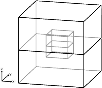
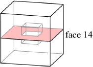
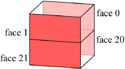
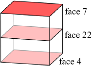
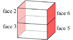
Figure 1: Schematic Diagram of the Cube-In-Cube Model. Figure (a) shows a schematic diagram of the cube-in-cube model. The inner cube is centered within the outer cube and has a length equal to 1/3 that of the outer cube. Figure (b) shows the numbering of the internal faces of the model. The upper-left figure shows the entire cube-in-cube model, while the rest show only the inner cube. In our simulation, we load the upper face of the model in the $z$-direction. Under such loading, faces 4, 7, 14, and 22 are subject to pure normal traction. Faces 0, 1, 2, 3, 5, 6, 20, and 21, are subject to pure shear traction. (The numbering of the internal faces is not contiguous because the finite element simulation also numbers the ten external faces.) The inner cube is a single crystal, but in order to allow for intragranular fracture through this crystal, we add an internal face through the center. The constitutive relation for this interface is that of a perfect crystal. Notice that pairs 0&1, 2&6, 3&5, and 20&21 are boundaries that macroscopically have identical cohesive laws since they are related by an inversion, i.e. they constitute symmetric pairs of interfaces for which the grains have been swapped.

2 The Cohesive Zone Model

The cohesive zone constitutive model is implemented in a finite element model with zero volume interface elements placed between the regular finite elements at interfaces. An example of an interface element is shown in Figure 2. These interface elements simulate fracture by debonding according to a cohesive law, the relation between the traction and displacement across the interface. The form of cohesive law used here is the piecewise linear form developed by Tvergaard and Hutchinson [15] also described by Gullerud et al. [16]. An example is shown in Figure 2. The piecewise linear form of the cohesive law is determined by the initial stiffness $k_{0}$, the peak traction $\tau_{p}$, and the critical displacement, $\delta_{c}$ at which the surface is considered fully debonded and traction-free.

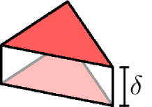
Figure 2: Interface Elements and the Piecewise Linear Cohesive Law. Figure (a) shows a schematic diagram of a triangular interface element. The displacement across the interface $\delta$, is initially zero. Each of the two triangles forms a face of one of the tetrahedral elements in the material on either side of the interface. Figure (b) shows the form of the constitutive relation for the interface elements. The slope of the first linear segment is the initial stiffness, $k_{0}$. When the traction across the interface reaches the peak traction, $\tau_{p}$, the interface element begins to soften. When the normalized displacement, defined by $\lambda=\delta/\delta_{c}$ reaches a value of 1, the interface has fully debonded.

Camacho and Ortiz [17] describe mixed loading by assigning different weights to the tangential and normal components of displacement, described by a factor $\beta$. We also assume that the resistance relative to tangential displacements is considered to be independent of direction. This leads to an effective displacement of

$$\delta=\sqrt{\delta_{n}^{2}+\beta\delta_{t}^{2}}$$ (1)

where $\delta_{n}$ is the normal displacement and $\delta_{t}$ is the tangential displacement. The effective traction is

$$\tau=\sqrt{\tau_{n}^{2}+\beta^{-2}\tau_{t}^{2}}$$ (2)

where $\tau_{n}$ is the normal component of traction and $\tau_{t}$ is the tangential component of traction.

3 Atomistically Determined Material Properties Used by CZM

The parameters needed by the CZM simulation that are determined by atomistics are the elastic constants associated with the atomic potential, the orientation of the lattice in each grain, and the cohesive law of each interface. We are modelling silicon using the Stillinger-Weber (SW) potential [18] but with an extra parameter, $\alpha$, multiplying the three body term such that $\alpha=1$ corresponds to standard SW. We use two values for this parameter, the standard value of 1.0 (matching to other properties of real silicon) and a value of 2.0 which makes the material more brittle. We calculate separate material properties (elastic constants and cohesive laws) for each version of SW.

3.1 Determining the Elastic Constants

In order to make a direct comparison between the atomistic and finite element (FE) simulations, we must determine the elastic constants of each version of SW for input into the FE simulation. The elastic constants are measured by initializing a cube of atoms in a diamond lattice, incrementing a strain in one direction, relaxing the atoms at zero temperature, and measuring the stress tensor at each increment.

For an interatomic potential with 3-body terms of the form

$$E_{i}=\sum_{j<k}f(\vec{r_{ij}},\vec{r_{ik}}),$$ (3)

we can find the $\alpha\beta$ component of stress at atom $i$ by utilizing the relation [19]

$$(\sigma_{i})_{\alpha,\beta}=\frac{1}{V}\frac{\partial E_{i}}{\partial\epsilon_{\alpha,\beta}}$$ (4)

where $V$ is the volume per atom. This leads to

$$(\sigma_{i})_{\alpha,\beta}=\frac{1}{V}\sum_{j<k}\frac{\partial E_{i}}{\partial\vec{r_{ij}}}\cdot\frac{\partial\vec{r_{ij}}}{\partial\epsilon_{\alpha,\beta}}+\frac{\partial E_{i}}{\partial\vec{r_{ik}}}\cdot\frac{\partial\vec{r_{ik}}}{\partial\epsilon_{\alpha,\beta}}.$$ (5)

Because

$$\partial(r_{ij})_{\gamma}/\partial\epsilon_{\alpha,\beta}=(r_{ij})_{\beta}\delta_{\alpha,\gamma},$$ (6)

the atomic stress is

$$(\sigma_{i})_{\alpha,\beta}=\frac{1}{V}\sum_{j<k}\frac{\partial E_{i}}{\partial(r_{ij})_{\alpha}}(r_{ij})_{\beta}+\frac{\partial E_{i}}{\partial(r_{ik})_{\alpha}}(r_{ik})_{\beta}.$$ (7)

We use a value of $V$ equal to the volume per atom in the ground state (perfect lattice). This has the shortcoming that for atoms near dislocations or grain boundaries, the actual volume per atom will be quite different.

$C_{11}$, $C_{12}$, and $C_{44}$ are determined by $\sigma_{xx}/\epsilon_{xx}$, $\sigma_{xx}/\epsilon_{yy}$, and $\sigma_{xy}/\epsilon_{xy}$, respectively. The results are given in Table 2. The differences between the elastic constants calculated for SW silicon and those found by experiement are due to the fact that the inter-atomic potential is an approximate representation of real silicon.

Table 2: Elastic constants of silicon, determined atomistically for two versions of SW silicon.

• 	Original SW (GPa)		Brittle SW (GPa)		Experiment [20] (GPa)
  $C_{11}$	69.	74	92.	78	166
  $C_{12}$	35.	20	23.	69	064
  $C_{44}$	52.	00	83.	37	080

3.2 Calculating the Cohesive Laws

The method for computing the cohesive law of a grain boundary with an atomistic simulation is described in [14]. Here we are measuring fully 3D grain boundary geometries. An example of a 3D grain boundary simulation is shown in Figure 3. In order to simulate grain boundaries of any geometry (not just geometries restricted by commensurability) we use constrained layers of atoms on the surfaces instead of periodic boundary conditions. Because SW contains three body terms, a layer thickness equal to twice the cutoff distance of the potential is needed to ensure that the free atoms are not subject to surface effects. There is a constrained zone for each face (atoms that are within a constrained zone width of a single exterior face), edge (atoms that are within a constrained zone width of exactly two exterior faces), and corner (atoms that are within a constrained zone width of three exterior faces). The atoms on the faces are constrained to not move perpendicular to the face, the atoms on the edge are constrained to move only parallel to the edge, and the atoms in the corners are totally fixed in position. These constraints simulate “rollered” boundary conditions. Each grain is 30 Å wide and normal strain increments are 0.005. At each strain increment, we displace “endcaps”, the constrained atoms adjacent to the external faces that are parallel to the $yz$-plane (indicated by the gray boxes in Figure 3). We relax the atoms and measure the $xx$ component of stress on the endcaps. An example of the stress-strain curve that results from such a simulation is shown in Figure 4.

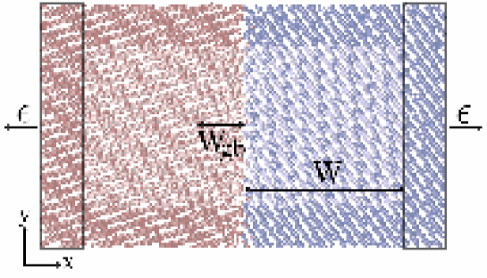
Figure 3: An Example of a Grain Boundary Simulation. The darker atoms represent constrained layer of atoms used to enforce rollered boundary conditions. The normal strain is imposed by displacing the constrained atoms on the endcaps which are indicated by the rectangles. $W$ is the width of the unconstrained atoms in each grain in the direction perpendicular to the interface. $W_{gb}$ represents the width of the strain field on either side of the interface, and is chosen such that (11) does not give a negative value.

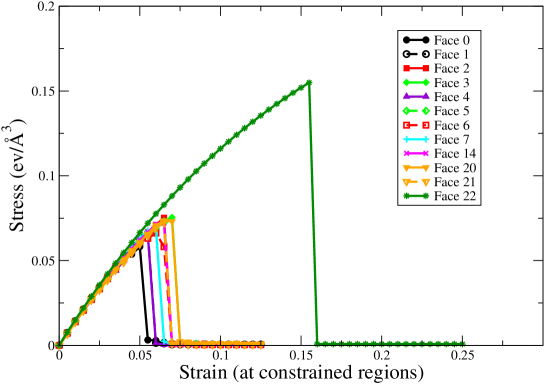
Figure 4: Strain versus Stress: Brittle SW Silicon. Strain versus stress for the twelve different interfaces needed for the continuum FE cube-in-cube simulation. Each grain is 30Å on a side. In order to calculate the cohesive law for only the grain boundary, we subtract off the elastic response of the bulk (Figure 5). Face 0 has no grain boundary, representing intragranular fracture through the center cube. Notice that the cohesive laws of the vertical interfaces are invariant under inversion, so some pairs of faces would have identical cohesive laws if measured in an infinite-sized system (or one with periodic boundary conditions and micro-parameters that are completely optimized). Thus the differences between faces 0&1, 2&6, 3&5, and 20&21, both here and in Figures 5,6, and 7 reflect the discreteness effects of the choice of lattice origin and positions of the edges of the simulation.

The CZM uses a traction-displacement law that describes the debonding at the interface in question [21, 17, 15] as discussed in section 2. The piecewise linear form is determined by the initial stiffness $k_{0}$, the peak traction $\tau_{p}$, and the final displacement $\delta_{c}$. We will need to extract these parameters from the output of our grain boundary simulation (Figure 4).

Because we are measuring the displacements 30 Å from the actual boundary, we need to subtract off the elastic response of the grain. Because we are using rollered boundary conditions, there is no Poisson-effect contraction, and the relevant component of the elastic tensor is $C_{1111}$, describing the strain normal to the grain boundary. The elastic tensor for the rotated crystal is found by rotating the elastic constants found in section 3.1 by the same rotation matrix that describes the rotation of the lattice vectors in each grain

$$C^{\prime}_{1111}=R_{1i}R_{1j}R_{1k}R_{1l}C_{ijkl}.$$ (8)

We must then combine $C^{\prime}_{1111}$ from each grain such that the stress in each grain is equal (analogous to springs in series)

$$\sigma=C^{(1)}_{1111}\frac{d_{1}}{W}=C^{(2)}_{1111}\frac{d_{2}}{W}=C^{\mathrm{eff}}_{1111}\frac{d_{1}+d_{2}}{2W}$$ (9)

$$C^{\mathrm{eff}}_{1111}=2/(\frac{1}{C^{(1)}_{1111}}+\frac{1}{C^{(2)}_{1111}})$$ (10)

where $d_{1}$ and $d_{2}$ refer to the displacement in each grain and $W$ is the width of each grain. The displacement near the grain boundary is then given by

$$d_{gb}=2W\epsilon-\frac{\sigma}{C^{\mathrm{eff}}_{1111}}2(W-W_{gb})$$ (11)

where $W_{gb}$ represents a finite width associated with the interface and $\epsilon$ is the external, normal strain. Since, in our system, the grain boundary is more stiff than the perfect crystal for the silicon geometries we have studied, this finite width is necessary so that (11) does not give a negative value. Figure 5 shows the result of applying this correction to the data show in Figure 4. The initial stiffness is then given by the peak stress divided by the displacement at peak stress. The final displacement is set such that the Griffith criterion is met, i.e. such that the area under the curve is equal to the difference between the final surface energies of the broken grain and the initial energy of the grain boundary interface, $\lambda_{c}=2(\gamma-\gamma_{gb})/\sigma_{c}$. Figures 6 and 7 show the final, piecewise linear cohesive laws that are used by the CZM simulations.

For the perfect crystal, we can simply scale the cohesive law to a width equal to the finite width used to process the grain boundary cohesive laws since we do not need to separate the behaviour of the bulk from the behaviour of an interface. This has the effect of preserving the non-linear elastic response. The non-linear elastic response of the bulk is not separated from the response of the interface for the case of grain boundaries, since the elastic response of the bulk that we subtract off is assumed to be linear. Since the grain boundaries have a lower fracture stress than the perfect crystal, nonlinear effects in the bulk are less important.

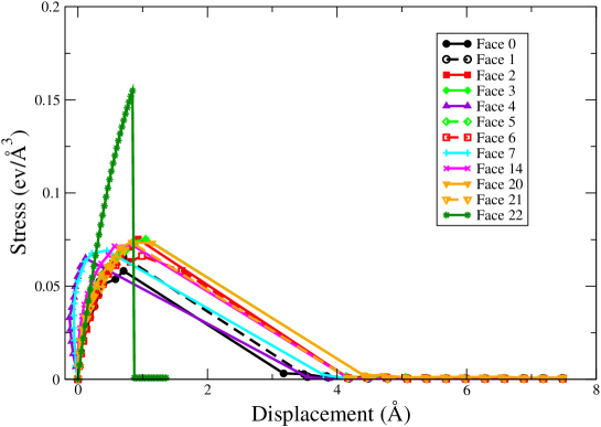
Figure 5: Cohesive Law: Brittle SW Silicon. Cohesive law, displacement versus stress, for the brittle potential and twelve interfaces of Figure 4. The transformation from strain to effective displacement at the interface is as described in section 3.2. The effective thickness of the interface is 9Å on each side. (Note that this is comparable to the entire size of the smaller atomistic cube-in-cube simulations.)

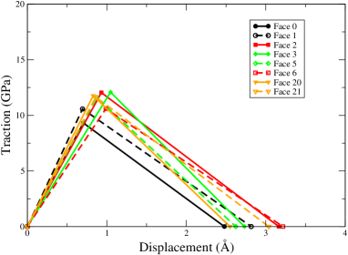
Figure 6: Piecewise Linear Cohesive laws: Brittle SW Silicon. Simplified piecewise linear cohesive law used in the FE simulations. The peak stress and its corresponding displacement were taken from Figure 5, and the critical displacement where the force vanishes is chosen to make the area under the curve equal the Griffith energy. In the figure on the left, solid and dashed line pairs of the same shade indicate pairs of interfaces with the same macroparameters (grain orientations) but different microparameters.

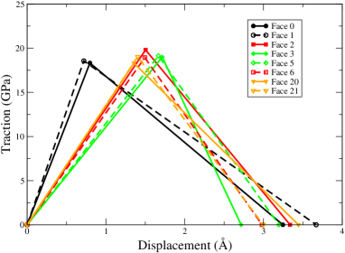
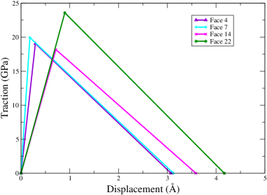
Figure 7: Piecewise Linear Cohesive laws: Ordinary SW Silicon. The same as Figure 6 but for the original, ductile SW potential for silicon.

In principle, two boundaries for which the grains have been swapped (such as faces 0&1, 2&6, 3&5, 20&21 as shown in Figure 1) should have the same overall structure and therefore have the same cohesive law. In practice, when simulating a finite region of a grain boundary, microparameters (the choice of section of the interface, the translations of the grains relative to one another, and the cutting plane of each lattice orientation) alter the grain boundaries that have the same macroparamters (grain orientation) or would otherwise be the same by symmetry. The differences between the cohesive laws for the pairs 0&1, 2&6, 3&5, 20&21 in figures 6 and 7 indicate the scope of this effect, of order 10% (much smaller than the discrepancy between atomistic and continuum simulations, which we will observe in section 5).

4 Fully Atomistic Simulation

The fully atomistic model is run with a software package called Overlapping Finite Elements and Molecular Dynamics (OFEMD) which is described in detail in [22, 23]. OFEMD uses the DigitalMaterial [24] library to run atomistic simulations of any geometry within a finite element mesh. OFEMD uses the mesh information to fill each material region with atoms in the given lattice orientation and set up contrained zones as described in section 3.2 to simulate rollered boundary conditions. The fully atomistic simulation uses the same kinematic boundary conditions as the FE simulation: a normal loading imposed on the upper face. We manually update the positions of the atoms in the constrained zones that are adjacent to the upper face to impose this boundary condition, incrementing the strain up to 15% in 0.5% strain increments, relaxing the atoms at each step.

5 Cohesive Zone Model Comparison

We compare the fracture behaviour of atomistic and continuum FE simulations for both the standard SW potential (which is ductile for single crystal, intragranular fracture) and the modified, brittle SW potential. We use both potentials to check if discrepancies between atomistic and continuum simulations could be due to ductility. We explore simulations of two sizes (inner cube sizes of 10 and 20Å) to check if discrepancies get smaller in the continuum limit of larger specimens. The interfacial cohesive laws in each case were computed as in Figures 6 and 7, from atomistic simulations with 30Å grains.

Figures 8 through 11 show the results of both the atomistic and continuum simulations for both versions of SW silicon and both length scales. The colour scales denote $\sigma_{zz}$, the vertical component of stress. The stresses for the atomistic simulations were calculated using (7). The first row of each figure shows the $xy$ center plane of the atomic simulation (roughly the plane of fracture). The second row shows the same plane of fracture for the CZM simulation. The third row shows the $xz$ center plane of the atomistic simulation, illustrating the stresses around the fracture zone and the crack opening. The fourth row shows the $xz$ center plane of the CZM simulation. The stress-free state, indicated by the colour blue, is an indication that decohesion has occurred across the interface within that region.

We shall see that the atomistic simulations and the FE simulations differ in several important respects. First, the FE simulations fracture overall at a higher strain level. This might be a nucleation effect; the irregular atomic structures at the external faces and internal edges and corners could be acting as nucleation points for fracture in ways that are not reflected in the continuum simulation. Second, the pattern of fracture—which interfaces break in which order—is in some cases different for the two simulations. Some of these differences are accidental; the system has inversion symmetries across the $xz$ and $yz$ planes that are broken only by the microparameter choices in the grain-boundary cohesive law atomistic simulations and the fully atomistic cube-in-cube simulations. The FE simulation reflects the choice of microparameters chosen in the cohesive law simulations while the fully atomistic simulation reflects another choice of microparameters. Hence an atomistic simulation that breaks first along the ‘front’ edge is equivalent to a FE simulation breaking along the ‘back’. Indeed, were we to use fully converged, infinite-system cohesive laws such as the periodic boundary conditions used in  [14], an ideal FE simulation would break symmetrically. However, this effect alone cannot account for the differences between the FE simulations and the fully atomistic simulations. We will see that these differences are larger than the differences due to microparameter choices (as observed in figures 6 and 7).

5.1 Brittle SW with a 10 Å Inner Cube

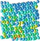
(a) 11%

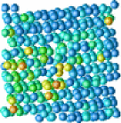
(b) 12%

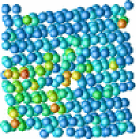
(c) 13%

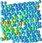
(d) 14%

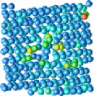
(e) 15%

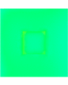
(f) 11.1%

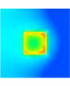
(g) 12.1%

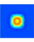
(h) 13.1%

(i) 14.1%

(j) 15.1%

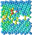
(k) 11%

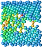
(l) 12%

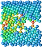
(m) 13%

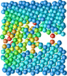
(n) 14%

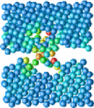
(o) 15%

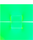
(p) 11.1%

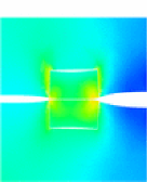
(q) 12.1%

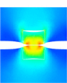
(r) 13.1%

(s) 14.1%

(t) 15.1%

Figure 8: Comparison of the Atomistic and CZM Simulations of the Cube-In-Cube with a 10 Å Inner Cube, using Brittle SW Silicon. The top two rows are $\sigma_{zz}$ on the $xy$ center (fracture) plane. The bottom two rows are $\sigma_{zz}$ on the $xz$ center, cross-sectional plane.

Figure 8 shows the comparison between the smaller simulations of the brittle potential (an inner cube length of 10Å, with the brittle modification of the SW potential). The atomistic simulation appears to begin to fracture at 11% strain in the upper right corner of the $xy$ plane in Figure 8(a) with the fracture spreading across the right side and finally across the center plane, extracting, rather than splitting, the inner cube at 15% strain. At this small scale, the inner cube is amorphized during the first relaxation step.

The finite element simulation begins to fracture on the right side as well between 11.1% strain and 12.1% strain, approximately where the atomistic simulation fractures. The only feature which breaks the 90 degree rotation symmetry for the finite element simulations are the differences in cohesive laws. The finite element simulation fractures slightly more rapidly, also ending by breaking through the inner cube but at 14.1% strain rather than 15%.

5.2 Brittle SW with a 20 Å Inner Cube

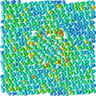
(a) 8%

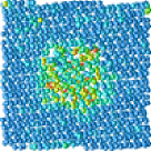
(b) 9%

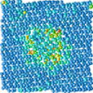
(c) 10%

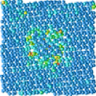
(d) 11%

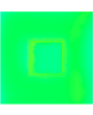
(e) 11.1%

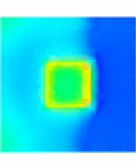
(f) 12.1%

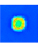
(g) 13.1%

(h) 14.1%

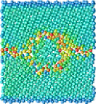
(i) 8%

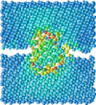
(j) 9%

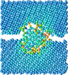
(k) 10%

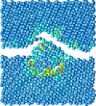
(l) 11%

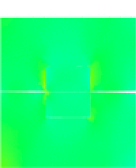
(m) 11.1%

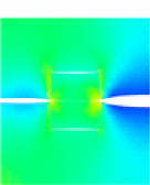
(n) 12.1%

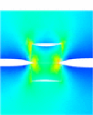
(o) 13.1%

(p) 14.1%

Figure 9: Comparison of the Atomistic and CZM Simulations of the Cube-In-Cube with a 20 Å Inner Cube, using Brittle SW Silicon. The top two rows are $\sigma_{zz}$ on the $xy$ center (fracture) plane. The bottom two rows areare $\sigma_{zz}$ on the $xz$ center, cross-sectional plane.

For the 20 Å length scale atomistic simulations (Figure 9), fracture also begins at the upper right corner of the $xy$ plane in Figure 9(a), however fracture begins noticeably earlier at 8% strain and propagates through the center plane more rapidly. At 9% strain, the atomistic simulation is comparable to the continuum simulation at 13% strain, with the center plane, excluding the inner cube, cracked through. This more rapid fracture of the atomistic simulation could be due to microstructure differences, but could also be due to the larger system size. A larger system height means there is more energy stored in elastic strain per unit area of interface. Once a given region reaches the maximum stress that it can sustain, it snaps open. With a smaller system size, the opening of the interface is controlled since the constrained zones are closer. This is related to the effect described in [14] where larger systems effectively approach fixed force boundary conditions.

Both the atomistic simulation and the finite element simulation begin to decohere at the upper face of the inner cube (compare Figure 9(k) with the slight blue decohered region above the inner cube in Figure 9(o)). However, the FE simulation ultimately decoheres at the center plane instead. In the atomistic simulation, we also see a competition between cracking at the top of the inner cube and cracking through the center plane. Ultimately, the crack propagates partially through the inner cube at an angle, reaching the top of the inner cube. This effect cannot be replicated in the finite element simulation because it did not have interface elements in position to crack at this angle.

5.3 Original SW with a 10 Å Inner Cube

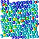
(a) 10%

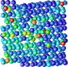
(b) 11%

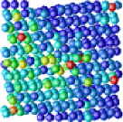
(c) 12%

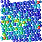
(d) 13%

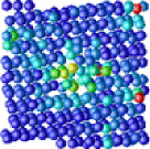
(e) 14%

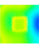
(f) 24.1%

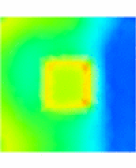
(g) 26.1%

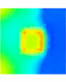
(h) 28.1%

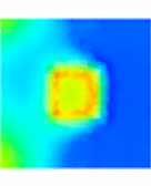
(i) 30%

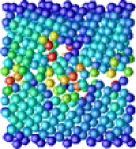
(j) 10%

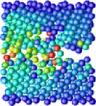
(k) 11%

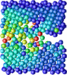
(l) 12%

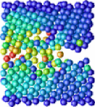
(m) 13%

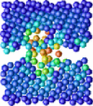
(n) 14%

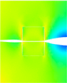
(o) 24.1%

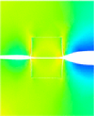
(p) 26.1%

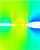
(q) 28.1%

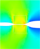
(r) 30%

Figure 10: Comparison of the Atomistic and CZM Simulations of the Cube-In-Cube with a 10 Å Inner Cube, using Original SW Silicon The top two rows are $\sigma_{zz}$ on the $xy$ center (fracture) plane. The bottom two rows are $\sigma_{zz}$ on the $xz$ center, cross-sectional plane.

For the original version of SW silicon (which is more ductile for single-crystal fracture) with the smaller inner cube size (Figure 10), the atomistic simulations fracture at around 14-15% strain, similar to the fracture threshold seen for the brittle potential atomistic simulations at that size. The continuum simulations, however, fracture at a much higher strain, 30% compared to 15%, despite using cohesive-zone models derived from the original potential.

The atomistic simulation begins to fracture at the top of the $xy$ plane (10% strain figure) and spreads along the right side (11, 12% figures). At the end of the atomistic simulation (14% strain), it has cracked through all but the center cube. The CZM simulation begins to fracture along the external edge along the side, and has also not cracked through or around the inner cube at the conclusion of the simulation.

5.4 Original SW with a 20 Å Inner Cube

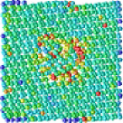
(a) 12%

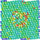
(b) 13%

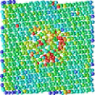
(c) 14%

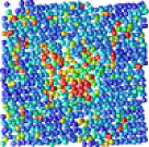
(d) 15%

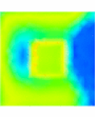
(e) 23.1%

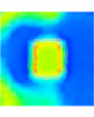
(f) 25.1%

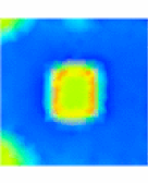
(g) 27.1%

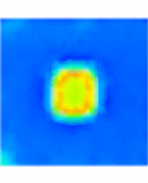
(h) 29.1%

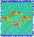
(i) 12%

(j) 13%

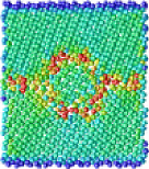
(k) 14%

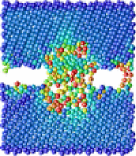
(l) 15%

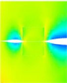
(m) 23.1%

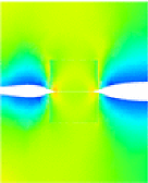
(n) 25.1%

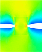
(o) 27.1%

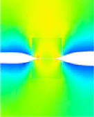
(p) 29.1%

Figure 11: Comparison of the Atomistic and CZM Simulation of the Cube-In-Cube with a 20 Å Inner Cube, using Original SW Silicon. The top two rows are $\sigma_{zz}$ on the $xy$ center (fracture) plane. The bottom two rows are $\sigma_{zz}$ on the $xz$ center, cross-sectional plane.

For the 20 Å case (Figure 11), the ductile atomistic simulation again fractures at a much lower stress than does the CZM simulation. The atomistic simulation fractures through all but the center cube very rapidly between 14% and 15% strain, reflecting again the effective soft-spring fixed-stress fracture conditions from the larger system size; the CZM simulation fractures more gradually, showing a sweep from right to left. The behaviour of the CZM simulation is similar to that of the 10 Å case with fracture beginning on the right side and slowly propagating through the center plane.

6 Conclusion

We have described a method for comparing finite element simulations of polycrystal models to fully atomistic simulations of the same geometry. In the finite element simulations, we used elastic constants and cohesive laws for the grain boundaries, derived from the atomistic calculations. We find fair agreement between the two simulations in one case (the 10 Å brittle SW simulation) in terms of the strain at which the fracture begins and the pattern of fracture. However, the more macroscopic, continuum, brittle simulation showed poor agreement, where one would have naively expected improved convergence. The more ductile simulations showed poor agreement at both length scales.

Some of the differences between the atomistic simulations and the finite element simulations can be attributed to the difference in choice of microparameters defining the grain boundary geometries (the location of the lattice origin with respect to the interface). Carefully matching these microparameters in future comparisons can only partially correct for the differences – there will always be discreteness effects in atomistic simulations that cannot be replicated in finite element simulations, due to the distortion of atoms at interface corners and junctions of grain boundaries. These sites, which are not described by cohesive laws, are often the locus for crack nucleation. In order to extract the cohesive properties of complex local regions, we suggest the use of direct, on-the-fly, locally atomistic simulations [22, 23].

References

References

- [1] A. Needleman. An analysis of tensile decohesion along an interface. Journal of the Mechanics and Physics of Solids, 38(3):289–324, 1990.
- [2] M. Falk, A. Needleman, and J. Rice. A critical evaluation of dynamic fracture simulations using cohesive surfaces. In Proceedings of the 5th European Mechanics of Materials Conference, Delft, 2001.
- [3] E. Iesulauro, A. R. Ingraffea, S. Arwade, and P. A. Wawrzynek. Simulation of grain boundary decohesion and crack initiation in aluminum microstructure models. In W. G. Reuter and R. S. Piascik, editors, Fatigue and Fracture Mechanics, volume 33, West Conshohocken, PA, 2002. American Society for Testing and Materials.
- [4] E. Iesulauro, A. R. Ingraffea, G. Heber, and P. A. Wawrzynek. A multiscale modeling approach to crack initiation in aluminum polycrystals. In 44th AIAA/ASME/ASCE/AHS Structures, Structural Dynamics, and Materials Conference, Norfolk, VA, April 2003. AIAA.
- [5] D. H. Warner, F. Sansoz, and J. F. Molinari. Atomistic based continuum investigation of plastic deformation in nanocrystalline copper. International Journal of Plasticity, 22:754–774, 2006.
- [6] S. P. Chen, D. J. Srolovitz, and A. F. Voter. Computer simulation on surfaces and [001] symmetric tilt grain boundaries in ni, al, and ni3al. Journal of Materials Research, 4:62, 1989.
- [7] R. J. Harrison, G. A. Bruggeman, and G. H. Bishop. Grain Boundary Structure and Properties, chapter Computer Simulation Methods applied to Grain Boundaries, pages 45–91. Academic Press Inc., London, 1976.
- [8] P. H. Pumphrey. Grain Boundary Structure and Properties, chapter Special High Angle Grain Boundaries, pages 139–200. Academic Press Inc., London, 1976.
- [9] F. Sansoz and J. F. Molinari. Mechanical behavior of tilt grain boundaries in nanoscale cu and al: A quasicontinuum study. Acta Materialia, 53:1931–1944, 2005.
- [10] O. A. Shenderova, D. W. Brenner, A. Omeltchenko, X. Su, and L. H. Yang. Atomistic modeling of the fracture of polycrystalline diamond. Phys. Rev. B, 61:3877–3888, 2000.
- [11] D. Wolf. Materials Interfaces: Atomic-level structure and properties, chapter Atomic-level geometry of crystalline interfaces, pages 1–52. Chapman & Hall, 1992.
- [12] D. Wolf and K. L. Merkle. Materials Interfaces: Atomic-level structure and properties, chapter Correlation between the structure and energy of grain boundaries in metals, pages 88–150. Chapman & Hall, 1992.
- [13] D. Wolf and J. A. Jaszczak. Materials Interfaces: Atomic-level structure and properties, chapter Role of interface dislocations and surface steps in the work of adhesion, pages 662–690. Chapman & Hall, 1992.
- [14] Valerie R. Coffman and James P. Sethna. Grain boundary energies and cohesive laws as a function of geometry. 2007. submitted.
- [15] Viggo Tvergaard and John W. Hutchinson. The relation between crack growth resistance and fracture process parameters in elastic-plastic solids. Journal of the Mechanics and Physics of Solids, 40(6):1377–1397, 1992.
- [16] Arne Gullerud, Kyle Koppenhoefer, Arun Roy, Sushovan RoyChowdhury, Matt Walters, Barron Bichon, Kristine Cochran, Adam Carlyle, and Robert H. Dodds Jr. Warp3d-release 15.6: 3d dynamic nonlinear fracture analysis of solids using parallel computers and workstations. Technical report, University of Illinois at Urbana-Champaign, 2006.
- [17] G. T. Camacho and M. Ortiz. Computational modelling of impact damage in brittle materials. International Journal of Solids and Structures, 33:2899–2938, 1996.
- [18] F. H. Stillinger and T. A. Weber. Computer simulation of local order in condensed phases of silicon. Phys. Rev. B, 31:5262, 1985.
- [19] John Price Hirth and Jens Lothe. Theory of Dislocations. John Wiley & Sons, New York, 1982.
- [20] J. deLaunay. Solid State Phys., 2:220, 1956.
- [21] X. P. Xu and A. Needleman. Numerical simulations of fast crack groth in brittle solids. Journal of the Mechanics and Physics of Solids, 42(9):1397–1434, 1994.
- [22] Valerie R. Coffman. Macroscopic Effects of Atomic Scale Defects in Crystals: Grain Boundary Fracture and Brittle-Ductile Transitions. PhD thesis, Cornell University, 2007.
- [23] Valerie R. Coffman and Nicholas Bailey. MDWebServices. http://www.lassp.cornell.edu/sethna/DM/mdwebservices/.
- [24] Nicholas Bailey, Thierry Cretegny, James P. Sethna, Valerie R. Coffman, Andrew J. Dolgert, Christopher R. Myers, Jakob Schiotz, and Jens Jorgen Mortensen. Digital material: a flexible atomistic simulation code, 2006, http://arxiv.org/abs/cond-mat/0601236.