A new method to separate star forming from AGN galaxies at intermediate redshift: The submillijansky radio population in the VLA-COSMOS survey

Abstract

We explore the properties of the submillijansky radio population at 20 cm by applying a newly developed optical color-based method to separate star forming (SF) from AGN galaxies at intermediate redshifts ($z\lesssim 1.3$). Although optical rest-frame colors are used, our separation method is shown to be efficient, and not biased against dusty starburst galaxies. This classification method has been calibrated and tested on a local radio selected optical sample. Given accurate multi-band photometry and redshifts, it carries the potential to be generally applicable to any galaxy sample where SF and AGN galaxies are the two dominant populations.

In order to quantify the properties of the submillijansky radio population, we have analyzed $\sim 2,400$ radio sources, detected at 20 cm in the VLA-COSMOS survey. $90\%$ of these have submillijansky flux densities. We classify the objects into 1) star candidates, 2) quasi stellar objects, 3) AGN, 4) SF, and 5) high redshift ($z>1.3$) galaxies. We find, for the composition of the submillijansky radio population, that SF galaxies are not the dominant population at submillijansky flux levels, as previously often assumed, but that they make up an approximately constant fraction of $30-40\%$ in the flux density range of $\sim 50~{}\mathrm{\mu}$Jy to $0.7$ mJy. In summary, based on the entire VLA-COSMOS radio population at 20 cm, we find that the radio population at these flux densities is a mixture of roughly $30-40\%$ of SF and $50-60\%$ of AGN galaxies, with a minor contribution ($\sim 10\%$) of QSOs.

1. Introduction

The most straight-forward information that can be derived from extra-galactic radio sky surveys are the radio source counts, which have been extensively studied in the last three decades (Condon, 1984; Windhorst et al., 1985; Gruppioni et al., 1999; Seymour et al., 2004; Simpson et al., 2006). If space was Euclidian, and there was no cosmic evolution of radio sources, then the differential source counts would follow a power law with exponent of $2.5$ (see e.g. Peterson 1997). Hence, the observed slope (and the change of the slope) of the radio source counts in different flux density ranges provides an insight, although quite indirect, into the global properties of extra-galactic radio sources, and their cosmic evolution. Past studies have shown that at 1.4 GHz flux densities above $\sim 100$ mJy the source counts are dominated by ’radio-loud’ AGN with luminosities above the Fanaroff & Riley (1974; FR) break ($\sim 2\times 10^{25}$ W Hz^-1; Willott et al. 2002). Decreasing from about $100$ mJy to $1$ mJy, the source counts follow a power law (e.g. Windhorst et al. 1985), and are mostly made up of ’radio-loud’ objects with luminosities below the FR break (FR Class I sources). However, the differential source counts change their slope again, i.e. they flatten below 1 mJy, and these sub-mJy radio sources have often been interpreted as a rising new population of objects, which does not contribute significantly at higher flux densities (e.g. Condon 1984).

To date the exact composition of this faint radio population (hereafter ’population mix’) is not well determined, and it is rather controversial. Windhorst et al. (1985) suggested that the majority of sub-mJy radio sources are faint blue galaxies, presumably undergoing significant star formation. Optical spectroscopy, obtained by Benn et al. (1993), supported this idea, and the source counts at faint levels were successfully modeled with a population of intermediate-redshift star forming galaxies (Seymour et al., 2004). However, spectroscopic results by Gruppioni et al. (1999) suggested that early-type galaxies were the dominant population at sub-mJy levels. Further, it was recently suggested and modeled that the flattening of the source counts may be caused by ’radio-quiet’ AGN (radio-quiet quasars and type 2 AGN), rather than star forming galaxies (Jarvis & Rawlings, 2004); observations support this interpretation (Simpson et al., 2006). Based from the combination of optical and radio morphology as an identifier for AGN and SF galaxies, Fomalont et al. (2006) suggested that at most $40\%$ of the sub-mJy radio sources are comprised of AGN, while Padovani et al. (2007) indicated that this fraction may be $60-80\%$ (the latter based their SF/AGN classification on a combination of optical morphologies, X-ray luminosities, and radio–to–optical flux density ratios of their radio sources).

Two main reasons exist for such discrepant results. First, the identification fraction of radio sources with optical counterparts, which is generally taken to be representative of the full radio population, spans a wide range in literature (20% to 90%) depending on the depth of both the available radio and optical data, as well as the passband used (e.g. a larger fraction of radio sources are associated with NIR than optical data; see Sec. 3.2). Second, the methods that were used to separate AGN from SF galaxies have been very heterogeneous in the past, ranging from pure radio luminosity or morphology cuts, through observed color properties to optical spectroscopy.

The two main populations of radio sources in deep radio surveys at 1.4 GHz (20 cm) are active galactic nuclei and star forming galaxies (Condon, 1984; Windhorst et al., 1985). At this frequency the radio emission predominantly arises from synchrotron emission powered either by accretion onto the central super-massive black hole (SMBH) or by supernovae remnants (e.g. Condon 1992, note that both mechanisms may be at work in a given galaxy). It was shown that radio properties such as the distributions of mono-chromatic luminosities of SF and AGN galaxies (Seyferts, LINERs) are comparable and overlapping (at least locally; e.g. Sadler et al. 1999). Hence, in order to disentangle SF and AGN galaxies in the radio regime, observations at other wavelengths are required.

Studies of extra-galactic radio sources in the local universe ($z<0.3$) have been invigorated due to the recent advent of panchromatic photometric and spectroscopic all-sky surveys, such as e.g. NVSS (Condon et al., 1998), FIRST (Becker et al., 1995), SDSS (York et al., 2000), IRAS (Beichman et al., 1985), 2dF (Colless et al., 2001) which provide additional panchromatic photometric (e.g. Simpson et al. 2006) and/or optical-IR spectroscopic (e.g. Sadler et al. 1999; Best et al. 2005a) observations. For example, the panchromatic properties of radio sources were studied to full detail (Ivezić et al., 2002; Obrić et al., 2006), as well as the environmental dependence of radio luminous AGN and SF galaxies (Best, 2004), and their luminosity function (Sadler et al., 1999; Jackson & Londish, 2000; Chan et al., 2004; Best et al., 2005a). Further, radio emission as a star formation rate indicator was well calibrated using a local sample (Bell, 2003) and compared to other star formation tracers (Hopkins et al., 2003).

However, it still remains to uncover the global properties of the intermediate-redshift ($z\lesssim 1.3$) radio sources. For example, the cosmic star formation history of the universe (i.e. the global star formation rate per unit comoving volume as a function of redshift) was not determined with a high accuracy using radio data (see e.g. Haarsma et al. 2000; Hopkins 2004), the radio luminosity function for SF and AGN galaxies at $z>0.3$ is not known, and the exact composition of the sub-millijansky radio population is still unknown and a matter of debate (Condon, 1984; Windhorst et al., 1985; Gruppioni et al., 1999; Seymour et al., 2004; Jarvis & Rawlings, 2004; Simpson et al., 2006).

In this work and in a number of accompanying papers, we will focus on these properties of radio sources using the 1.4 GHz VLA-COSMOS survey (Schinnerer et al., 2007). The main aim of the current paper is twofold. First, we develop a method based only on multi-wavelength photometric data to efficiently separate SF from AGN galaxies in the VLA-COSMOS 20 cm survey. Secondly, we use this classification to derive the composition of the sub-mJy radio population. In Sec. 2 we describe the COSMOS multi-wavelength data, and in Sec. 3 we present the cross-correlation of the sources detected at 1.4 GHz with catalogs at other wavelengths. In Sec. 4 we describe our source classification methodology and introduce our ’rest-frame color based classification method’ (see below), which we calibrate and extensively test using a large well-characterized sample of local galaxies. We present the classification of the VLA-COSMOS 1.4 GHz radio sources with identified optical counterparts in Sec. 5, and in Sec. 6 we compare our classification method with other classification schemes proposed in the literature. In Sec. 7 we study the ’population mix’ in the VLA-COSMOS radio survey, based on the entire sample of VLA-COSMOS radio sources. We summarize our results in Sec. 8.

Throughout the paper we report magnitudes in the AB system, and assume the following cosmology: $H_{0}=70,\,\Omega_{M}=0.3,\Omega_{\Lambda}=0.7$. We define the radio synchrotron spectrum as $F_{\nu}\varpropto\nu^{-\alpha}$, and assume $\alpha=0.8$ if not stated otherwise. Hereafter, we refer to our method to classify the VLA-COSMOS radio sources into five sub-types of objects (star candidate, QSO, AGN, SF, high-z galaxy) as “classification method”, and to our method to disentangle only the SF from AGN galaxies, based on rest-frame color properties, as “rest-frame color based selection method”.

2. The multi-wavelength data set

In this section we describe the COSMOS multi-wavelength data used for the work presented here.

2.1. Radio data

The COSMOS field was observed at $1.4$ GHz ($20$ cm) with the NRAO Very Large Array (VLA) in A- and C- configuration (VLA-COSMOS Large Project; for details see Schinnerer et al. 2007). The final map, encompassing 2$\Box^{\circ}$, has a resolution of $1.5^{\prime\prime}\times 1.4^{\prime\prime}$, and a mean $rms$ of $\sim 10.5~{}[15]$ $\mu$Jy/beam in the central 1 [2]$\Box^{\circ}$.

The VLA-COSMOS source catalog reports the peak and total (i.e integrated) flux density for each object. For extended sources the total flux density is derived by integrating over the object’s size (see Schinnerer et al. 2007 for details), while for unresolved sources it is set to be equal to the peak flux density. Bondi et al. (2007) have shown that bandwidth smearing effects (i.e. chromatic aberration), combined with the pointing layout of the VLA-COSMOS observations, systematically decrease the measured source’s peak flux density to $\sim 80\%$ of its true value, while the total flux density remains unaffected. Therefore, to correct for this, all peak flux densities in the catalog need to be increased by 25%. However, such an effect further entails a necessary re-definition of the sources in the field considered to be unresolved (cf. Fig. 14 in Schinnerer et al. 2007 and Fig. 2 in Bondi et al. 2007). Therefore, to properly correct for bandwidth smearing effects, we have re-selected the unresolved sources following Bondi et al. (2007), and set their total flux densities to be 1.25 times their peak (respective integrated) flux densities. Throughout the paper we will use the integrated flux density, corrected for bandwidth smearing where needed, as the representative flux density for each source.

In order to minimize the number of possible spurious radio sources ($\sim 50\%$ below $5\sigma$), we select only objects from the catalog that were detected at a signal to noise of $\geqslant 5$, and are located outside regions contaminated by side-lobes from nearby bright sources. This yields 2388 (out of $3643$; i.e. $\sim 65\%$) sources, 78 of which consist of multiple components.

2.2. Near-ultraviolet, optical and infrared imaging data

The NUV to MIR imaging data and photometry for the COSMOS survey used here include data taken during 2003–2006 with ground – (Subaru, KPNO, CTIO, CFHT) and space (HST, Spitzer) – based telescopes, covering a wavelength range from 3500 Å to 8 $\mu$m, described them in more detail below.

2.2.1 Ground-based data

The data reduction of the COSMOS ground-based observations in 15 photometric bands ranging from NUV to NIR, and the generation of the photometric catalog, is presented in Capak et al. (2007) and Taniguchi et al. (2007a). Here we make extensive use of the COSMOS photometric catalog. The photometric catalog was selected using the $0.6^{\prime\prime}$ resolution $i^{+}$ image. However, the photometry was obtained from the PSF (point-spread function) matched images, which degrades the resolution to $\sim 1.8^{\prime\prime}$. The median $5\sigma$ depths in AB magnitudes in the catalog for the $u^{*}$, $B_{J}$, $g^{+}$, $V_{J}$, $r^{+}$, $i^{+}$, $i^{*}$, $z^{+}$ and $K_{s}$ bands are 26.4, 27.3, 27.0, 26.6, 26.8, 26.2, 24, 25.2 and 21.6, respectively (see also tab. 2 in Capak et al. 2007). It is noteworthy that the detection completeness of the catalog is above $87\%$ for objects brighter than $i=26$.

2.2.2 Space-based data

The HST/ACS observations, which covered 1.8$\Box^{\circ}$ of the 2$\Box^{\circ}$ COSMOS field, are described in Scoville et al. (2007a) and Koekemoer et al. (2007). The F814W band imaging has a resolution of $0.09^{\prime\prime}$ and a $5\sigma$ point-source sensitivity of $I_{AB}=28.6$ (see also Capak et al. 2007). The ACS source catalog, which we utilize here, was constructed by Leauthaud et al. (2007), with special care given to the separation of point-sources from extended objects.

The Spitzer observations of the COSMOS field in all seven bands (3.6, 4.5, 5.8, 8.0, 24, 70, 160 $\mu$m) are described in Sanders et al. (2007). The 3.6 – 8 $\mu$m band catalog is available to full depth for the entire field. The resolution in the 3.6, 4.5, 5.8, 8.0 $\mu$m bands is $1.7^{\prime\prime}$, $1.7^{\prime\prime}$, $1.9^{\prime\prime}$, and $2^{\prime\prime}$, respectively. The catalog was generated using SExtractor on the four IRAC channels in dual mode, with the 3.6 $\mu$m image as the detection image. The $5\sigma$ depth for point-sources at 3.6 $\mu$m is 1 $\mu$Jy, corresponding to an AB magnitude of 23.9. In this work we also make use of the MIPS 24 $\mathrm{\mu}$m catalog obtained from the shallow observations of the entire COSMOS field during Cycle 2 of the S-COSMOS program (see Sanders et al. 2007 for details). The resolution and $5\sigma$ depth of the catalog are $6^{\prime\prime}$ and 0.3 mJy, respectively. The latter corresponds to an AB magnitude of $17.7$. For the purpose of this paper, we will use only sources that were detected at 24 $\mathrm{\mu}$m at or above the $3\sigma$ level corresponding to their local rms.

2.3. X-ray data

The full 2$\Box^{\circ}$ COSMOS field was observed with the XMM-Newton satellite EPIC camera for a total net integration time of 1.4 Ms (for a description of the XMM-COSMOS survey see Hasinger et al. 2007). The limiting flux density of the XMM-COSMOS survey is $10^{-15}$ erg cm^-2 s^-1 and $5\times 10^{-15}$ erg cm^-2 s^-1 in the soft ($0.5-2$ keV) and hard ($2-10$ keV) bands, respectively. The X-ray point-source detection is described in Cappelluti et al. (2007), and the optical identifications of the X-ray sources for the first 12 observed XMM fields (over a total of 1.3$\Box^{\circ}$) are presented by Brusa et al. (2007a). For the analysis presented here we utilize the catalog with 1865 optical counterparts of the XMM-COSMOS point sources, drawn from the full 2$\Box^{\circ}$ XMM-Newton mosaic (Brusa et al., 2007b).

2.4. Photometric redshifts

The COSMOS photometric redshifts (Ilbert et al., 2007) utilized here are based on an a large amount of deep multi-color data (Capak et al., 2007b; Taniguchi et al., 2007a, b): 6 broad optical bands obtained at the Subaru telescope ($u^{+}$, $g^{+}$, $r^{+}$, $i^{+}$, $z^{+}$) and 2 at CFHT ($u^{*}$ and $i^{*}$), 8 intermediate and narrow band filters from the Subaru telescope ($IA427$, $IA464$, $IA505$, $IA574$, $IA709$, $IA827$, $NB711$, $NB816$), deep $Ks$-band data from the WIRCAM/CFHT camera (McCracken et al., in prep), and $3.6\mu m$ and $4.5\mu m$ data from the SPITZER IRAC camera (Sanders et al., 2007). The photometric redshifts are estimated via a standard $\chi^{2}$ fitting procedure (Arnouts et al., 2002) using the code Le Phare written by S. Arnouts & O. Ilbert. A major feature of this method is the calibration of the photometric redshifts using a spectroscopic sample of $\sim 1000$ bright galaxies ($I_{AB}<22.5$) obtained as part of the zCOSMOS survey (Lilly et al., 2007). We follow exactly the same calibration method as described in Ilbert et al. (2006): a) a calibration of the photometric zero-points, and b) an optimization of the template SEDs (spectral energy distributions). This calibration method allows us to remove systematic offsets in the estimates of the photometric redshifts. A direct comparison between the photometric redshifts and the zCOSMOS spectroscopic redshifts shows that the photometric redshifts reach an accuracy of $\sigma\left(\frac{\Delta z}{1+z}\right)\sim 0.014$ at $i<22.5$. The fraction of catastrophic failures is less than 1% at $i<22.5$. Such an accuracy and robustness can be achieved thanks to both the intermediate bands and deep NIR photometric data. The photometric redshifts for the entire COSMOS population will be described in full detail in Ilbert et al. (2007). The galaxies in the sample used here are radio selected, i.e. they are not randomly drawn from the global COSMOS population. Therefore, in Fig. 1 we show the comparison of the photometric and spectroscopic redshifts for a sub-sample of our VLA-COSMOS sources with available spectroscopy (see next section). The accuracy is $\sigma\left(\frac{\Delta z}{1+z}\right)=0.027$, which is somewhat lower than the accuracy for the full sample of COSMOS sources, however it is still satisfactory.

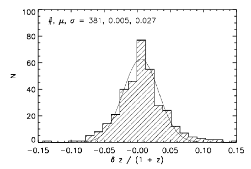
Figure 1.— The comparison of the photometric and spectroscopic redshifts for the VLA-COSMOS radio sources with optical counterparts (see Sec. 3.1) for which spectroscopy is available. The distribution shown was limited to spectroscopic redshifts $\leq 1.3$, consistent with the redshift range used in this work. The number of sources ($\#$), mean ($\mu$), and standard deviation ($\sigma$) of the distribution are indicated in the top left of the panel. Note the excellent accuracy of the photometric redshifts.

As photometric redshift codes generally take into account only galaxy SED models, the photometric redshifts for broad line AGN are usually poorly estimated (not better than $\sigma\left(\frac{\Delta z}{1+z}\right)\sim 0.1$ with a large fraction of catastrophic outliers and no solutions found beyond $z\sim 1.1$), and alternative ways for their redshift computations have to be applied. At the time of writing, no accurately estimated photometric redshifts for broad line AGN exist for the COSMOS project. The photometric redshifts for broad line AGN will be presented in a future publication (Salvato et al., 2007).

2.5. Optical spectroscopic data

The ongoing COSMOS optical spectroscopic surveys (Trump et al., 2007; Impey et al., 2007; Lilly et al., 2007) provide to date $657$ spectra, with good redshift estimates, for objects in the VLA-COSMOS 1.4 GHz radio sample described in Sec. 2.1. We augment this spectroscopic data set with available spectroscopic information for $65$ galaxies from the SDSS DR4 “main” spectroscopic sample, $13$ objects from the SDSS DR5 quasar catalog (Schneider et al., 2005), $2$ sources from the 2dF survey, as well as for $27$ objects taken with the MMT $6.5$ m telescope, and presented by Prescott et al. (2006). Thus, a total of $764$ spectra is available. However, as a number of sources were spectroscopically observed multiple times, we have spectroscopic information for $520$ unique sources in our radio sample. Throughout the paper, we use the spectroscopic redshifts, where available. We also use this sub-set of radio sources with observed optical spectra as a control sample to verify the presented classification method.

3. VLA-COSMOS 1.4 GHz radio sources at other wavelengths

In this section we define the ’matched’ radio source sample, a sample of radio sources with optical counterparts cross-correlated with the panchromatic COSMOS observations, as well as the ’remaining’ radio source sample, both of which will be used throughout the paper. First, we restrict the full VLA-COSMOS radio source sample to objects which have optical counterparts (Sec. 3.1). Then we positionally match these objects with sources detected in the MIR (Sec. 3.2) and X-ray (Sec. 3.3) spectral ranges. In Sec. 3.4 we describe the remaining radio sources that are either without identified or with identified but flagged optical counterparts.

3.1. Positional matching of the COSMOS radio and NUV/optical/NIR catalogs

The VLA-COSMOS Large Project source catalog contains 2388 radio sources detected at a signal to noise $\geqslant 5$ and outside side-lobe-contaminated regions (see Sec. 2.1). $78$ of these consist of multiple components. For the purpose of this paper we match these radio sources with sources that have also been detected in the optical regime, and are reported in the COSMOS photometric catalog (Capak et al., 2007). In order to obtain a sample with reliable radio-optical counterparts, we positionally match the radio sources only with optical sources brighter than $i=26$. The reason for this is illustrated in Fig. 2, where we show the distance between the radio sources and their nearest optical counterparts as a function of the $i$ band magnitude. As the median distance rapidly increases for $i>26$ (most probably introducing a significant number of false match associations) we apply a cut of $i=26$ to the NUV-NIR photometric catalog before matching the radio and optical catalogs.

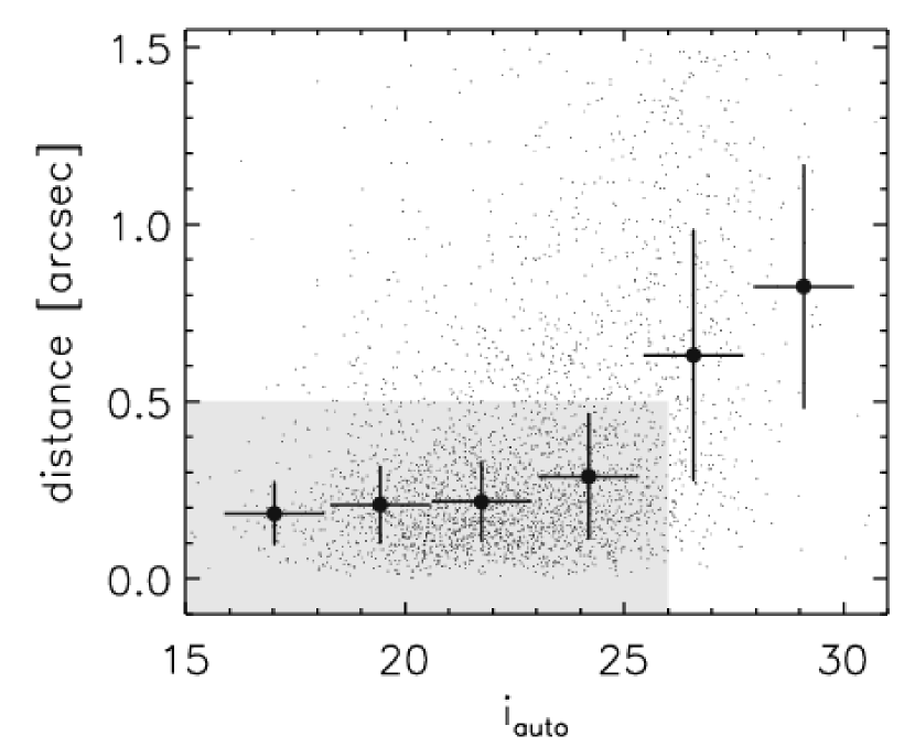
Figure 2.— Distance as a function of $i$ band magnitude for radio sources in the VLA-COSMOS survey (with $\mathrm{S/N}\geq 5$) positionally matched to the closest optical counterpart (small dots). The large dots show the median distance for each magnitude bin (the width of the bin is indicated by horizontal lines) and the corresponding interquartile range (vertical lines). Note that the median distance is significantly larger beyond $i=26$, presumably introducing a significant number of false match associations. The shaded area indicates the allowed matching region, which is set by the matching radius ($0.5^{\prime\prime}$) and the magnitude cut-off ($i=26$) used to find secure optical counterparts for the radio sources in the sample (see text for details).

Hence, to find the corresponding optical counterpart for each radio source (excluding multi-component sources, which are separately addressed below), we search for the nearest optical neighbor within a radial distance of $0.5^{\prime\prime}$. The search radius was chosen in such a way that it balances a high completeness of true matches and a low false-match contamination rate: A cut-off of $0.5^{\prime\prime}$ essentially includes all true matches in the sample, with a false association rate (computed from the source density in the matched catalogs) of only $\sim 4\%$. The high completeness and low contamination are due to the excellent astrometric accuracy of both the COSMOS radio and optical data. Our matching yielded 1749 radio sources with securely identified optical counterparts. However, 252 ($\sim 15\%$) of these are located in masked-out regions (i.e. around bright saturated stars) in the photometric catalog. Thus, their NUV-NIR photometry, as well as the photometric redshift computation has a significantly reduced accuracy. We exclude these objects from our main sample.

The multi-component radio sources in the VLA-COSMOS survey consist of radio sources which could not be fitted using a single Gaussian function (see Schinnerer et al. 2007). The radio morphologies of such sources can be fairly complex (e.g. single or double lobed radio galaxies), and this makes it substantially more difficult to associate such radio sources with the appropriate optical counterparts (see e.g. Ivezić et al. 2002; Best et al. 2005a). In order to avoid any biases which may be caused using an automatic association procedure, the optical counterparts of the VLA-COSMOS multi-component radio sources were determined visually. The 1.4 GHz catalog contains 78 multi-component sources detected at or above $5\sigma$, and 65 were securely associated with an optical counterpart with $i<26$, however 4 are located inside masked-out areas (around bright saturated stars) in the photometric catalog, and we therefore exclude them from the main sample.

In summary, the applied matching criteria yield 1814 ($\sim 76\%$ of the 2388 radio sources with $\mathrm{S/N}\geq 5$) radio sources with secure optical counterparts down to $i=26$, 65 of which are multiple component sources. The most accurate NUV-NIR photometry (i.e. excluding flagged regions around saturated objects) was obtained for 1558 ($\sim 86\%$ of 1814), 61 of which are multiple-component radio sources. Hereafter, we refer to this latter sample of 1558 radio sources, which make up $\sim 65\%$ of the radio sources with $\mathrm{S/N}\geq 5$, and that were matched to the NUV-NIR catalog, as the ’matched’ radio source sample. For reference, the 1.4 GHz total flux density distributions for the complete radio sample, the matched radio sample, and the sub-sample with available spectroscopy is shown in the top panel in Fig. 3. The distribution of the $i$ band magnitude for the matched radio sample, as well as the spectroscopic sub-sample, is shown in the bottom panel in Fig. 3. It is also worth noting that our cross-correlation is consistent with the results of the maximum likelihood ratio technique applied to VLA-COSMOS sources (Ciliegi et al., 2007a), however our restrictions for the masked-out regions in the photometric catalog, as well as the optical magnitude limit, are more conservative, as the analysis presented here strongly relies on accurate NUV to NIR photometry.

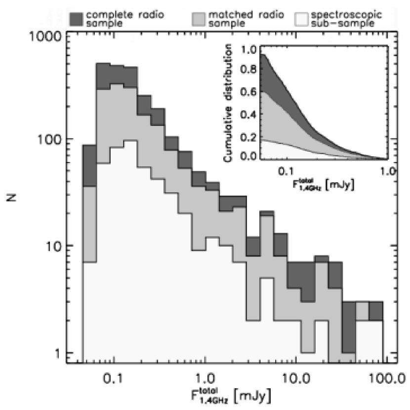
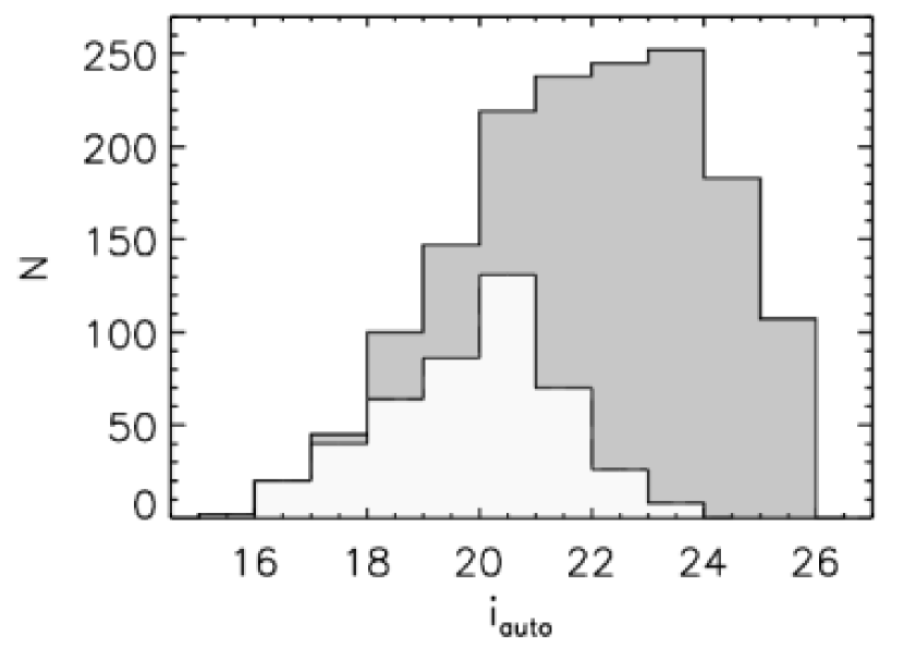
Figure 3.— Top panel: The distribution of the total 1.4 GHz (20 cm) flux density for i) the complete radio source sample ($\mathrm{S/N}\geq 5$; dark-grey shaded histogram), ii) the matched radio sample (grey-shaded histogram) and iii) the spectroscopic sub-sample (light-grey shaded histogram). The inset shows the cumulative distribution for the three samples computed as a function of decreasing total flux. Note that the spectroscopic sub-sample fairly represents the faint radio population as a function of the total flux. Bottom panel: Distribution of the $i$ band magnitude (Subaru where available, otherwise CFHT) for sources in the VLA-COSMOS matched radio source sample, and the spectroscopic sub-sample in the same notation as in the top panel.

A further data set that we use in the analysis presented here is the HST/ACS point-source information. We extract this information for each radio source in our matched sample by positionally matching the optical counterparts of the radio sources with point-sources identified in the HST/ACS F814W source catalog (Leauthaud et al., 2007). Using a matching radius of $0.5^{\prime\prime}$ yields 47 objects in our matched radio sample classified as point sources based on the HST/ACS F814W images. The mean distance between the matched objects is only $(0.12\pm 0.07)^{\prime\prime}$.

3.2. Radio – optical sources with IRAC and MIPS detections

We cross-correlate the matched radio source sample with the S-COSMOS – IRAC catalog using a maximum allowed distance to the optical counterparts of our radio sources of $0.5^{\prime\prime}$. [Note that such a cross-correlation allows for a maximum distance between the radio and MIR sources to be $1^{\prime\prime}$.] Such an adopted search radius essentially selects a complete radio – optical – MIR sample with a false match association for the MIR sources of $\lesssim 1$% with the optical counterparts, and $\lesssim 4$% with the radio counterparts. In summary, out of 1558 radio sources in the matched radio sample, $1448$ ($93\%$) have secure MIR counterparts.

The 24 $\mathrm{\mu}$m flux densities for all our radio sources were obtained from the COSMOS field observations using the S-COSMOS – MIPS shallow survey with a resolution of $6^{\prime\prime}$. Although a relaxed search radius of $5^{\prime\prime}$ was used to find the radio – 24 $\mathrm{\mu}$m counterparts, the median distance is only $0.19^{\prime\prime}$ with an interquartile range of $0.16^{\prime\prime}$. About $50\%$ (799 out of 1558) sources in the matched radio sample have a MIPS counterpart at 24 $\mathrm{\mu}$m with a signal to noise at or above 3.

3.3. Radio – optical sources with point-like X-ray emission

Using the maximum likelihood ratio technique Brusa et al. (2007a) presented the optical identifications of the X-ray point-sources (Cappelluti et al., 2007) detected in the XMM-COSMOS survey (Hasinger et al., 2007). Here we utilize their identifications to match the sources in our matched radio sample with detected X-ray point sources. Out of 1558 radio sources with optical counterparts, 179 ($12\%$ of 1558) are identified as point-sources in the X-ray bands. 17 of these have multiple counterpart candidates as defined by Brusa et al. (2007a). In these cases, if we assume that the radio sources are physically associated with the X-ray sources, then the radio data, which have a significantly better astrometric accuracy, can be used to constrain more precisely the optical counterpart of this given object. A visual inspection of the 17 sources, classified as having ambiguous identifications by Brusa et al. (2007b), strongly suggests that their most probable optical counterparts, reported in the X-ray – optical catalog, are real associations. Hence, we proceed in our analysis taking all 179 X-ray detected point sources to be true counterparts of the objects in the matched radio sample.

3.4. Radio sources with photometrically flagged or without optical counterparts at other wavelengths

In Sec. 3.1 we have defined the matched radio sample which consists of 1558 1.4 GHz sources that have optical counterparts out to an $i$ band magnitude of 26, and within a radial distance of less than $0.5^{\prime\prime}$. These sources were also required to have the most accurate NUV-NIR photometry, i.e. counterparts within flagged regions due to saturation and blending effects in the NUV-NIR images were excluded. Thus, 830 radio sources remain with no identified optical counterparts within these limits, 256 (i.e. $\sim 30\%$) of which have counterparts with $i\leq 26$ that lie in masked-out regions. Hereafter, we will refer to this sample of sources as the ’remaining radio source sample’. We positionally match these sources to the IRAC catalog using a maximum allowed distance of $1^{\prime\prime}$, and find 610 ($\sim 75\%$) matches. Based on Poisson statistics and the source density of the MIR sources, such a search radius essentially includes all true matches with a false contamination rate of $\lesssim 4$%. It is worth noting that more than one half of the remaining $25\%$ of the radio objects were independently identified as possible spurious sources, based on visual inspection, while the other half are either located in blended regions in the IRAC images or slightly further away than the allowed $1^{\prime\prime}$ from the position reported in the IRAC catalog (the morphology of the IRAC sources being often extended). Thus, we consider these $\sim 75\%$ of radio – MIR matches representative of the entire remaining radio population. Out of the 830 sources 318 (i.e. $\sim 40\%$) have MIPS 24 $\mathrm{\mu}$m detections ($\mathrm{S/N}\geq 3$), and 31 ($\sim 4\%$) have XMM point source counterparts (these 31 objects are a sub-sample of the 256 objects in the flagged regions). In Sec. 7 we analyze the properties of these remaining sources, and their contribution to the ’population mix’ in the VLA-COSMOS survey. The summary of the multi-wavelength cross-correlation of the VLA-COSMOS radio sources is given in Tab. 1.

4. Classification methodology

Extragalactic radio sources consist of two main populations: star forming and AGN galaxies. We further divide the AGN class into two sub-classes: QSOs (often unresolved in optical images, with broad emission lines in their spectra and high optical luminosity) and objects where the AGN does not dominate the entire SED, such as Type 2 QSOs, low-luminosity AGN (Seyfert and LINER galaxies) and absorption-line AGN (resolved in optical images, with both broad, narrow or no emission lines in their optical spectra). Throughout the paper, we will mostly refer to the latter sub-class only as ’AGN’.

The commonly adopted and well-calibrated tool for disentangling SF galaxies from low-luminosity AGN (Seyfert and LINERs) is the optical spectroscopic diagnostic diagram (Baldwin, Phillips & Terlevich, 1981), that is based on two emission line flux ratios ([OIII 5007]/H$\beta$ vs. [NII 6584]/H$\alpha$; hereafter BPT diagram; see also Veilleux & Osterbrock 1987; Rola, Terlevich & Terlevich 1997; Kewley et al. 2001). This diagnostic tool has been extensively used in the past for a successful separation of local SF and AGN galaxies (Sadler et al., 1999; Kauffmann et al., 2003; Brinchmann et al., 2004; Obrić et al., 2006; Smolčić et al., 2006). However, as spectroscopic observations are very expensive in terms of telescope time, especially when large numbers of faint objects need to be observed, alternative methods for the separation of SF from AGN galaxies, that eliminate the need for spectroscopy, have to be invoked. Here we develop such a method (hereafter ’rest-frame color based classification method’), which we apply in the next sections to identify SF and AGN galaxies in the VLA-COSMOS matched radio sample. The main idea of our method is drawn from the findings that the overall NUV to NIR SED of galaxies is a one-parameter family, and that spectral diagnostic parameters, such as line strengths, appear to be well correlated with the overall galaxy’s SED (see Obrić et al. 2006; Smolčić et al. 2006). In particular, Smolčić et al. (2006) have found a tight correlation between rest-frame colors of emission-line galaxies and their position in the BPT diagram. This correlation thus provides a powerful tool for disentangling SF from AGN galaxies using only photometric data, i.e. rest-frame colors, and we utilize it as the key of our rest-frame color based classification method.

4.1. Calibration of the rest-frame color based classification method in the local universe

4.1.1 The local spectroscopic sample

In order to obtain insight into the efficiency of the classification method, based on the rest-frame color ($P1$; see below), we construct a large sample of well-known low-redshift galaxies ($0.01<z<0.3$), whose properties are assumed to present well the properties of the galaxies in the VLA-COSMOS matched radio sample. The local sample was generated from the SDSS main galaxy sample, positionally matched to sources detected in the 1.4 GHz NVSS survey. Additionally, a sub-sample of galaxies detected with IRAS was constructed (see Obrić et al. 2006 for details about the cross-correlation of the SDSS, NVSS, IRAS catalogs). The SDSS/NVSS sample contains 6966 galaxies and the SDSS/NVSS/IRAS sample 875 galaxies with available SDSS optical spectroscopy. The computation of rest-frame colors ($P1$,$P2$) for these galaxies is presented in Smolčić et al. (2006). The rest-frame colors $P1$ and $P2$ optimally quantify the distribution of galaxies in the rest-frame color-color space. They are derived from the modified Strömgren photometric system ($uz$,$vz$,$bz$,$yz$ encompassing the wavelength range of 3200 – 5800Å; Odell et al. 2002, see also ) via a 2-dimensional principle component analysis in color-color space. A more detailed description of the colors, including their equational form, is given in Appendix A.

It is noteworthy to mention that given a) the detection limits, and b) the areal coverage of the NVSS and VLA-COSMOS surveys, both surveys observe approximately the same populations of objects, although over different redshift intervals (see Fig. 1 in Schinnerer et al. 2007). Assuming that evolutionary effects with redshift do not significantly alter the reliability of the identification method presented below, at least out to $z=1.3$, this makes the local sample of galaxies representative of the galaxies in the VLA-COSMOS matched radio sample.

Based on spectral line properties we separate the local sample into three classes of objects: AGN, star-forming galaxies and composite objects, where the latter are considered to have a comparable contribution of both star formation and AGN activity. First, galaxies with emission lines in their spectra are separated into these three classes using their position in the BPT diagram (see bottom panel in Fig. 4). Second, as the galaxies that have no emission lines in their spectra cannot be star forming (see also Sec. 4.1.3 for a discussion of this point), and as all of the objects in the SDSS/NVSS sample are observed to have 1.4 GHz emission which arises either from AGN or star formation activity in a galaxy, we define galaxies without emission lines in their spectra as AGN (see also Best et al. 2005a who classified these types of objects as absorption line AGN).

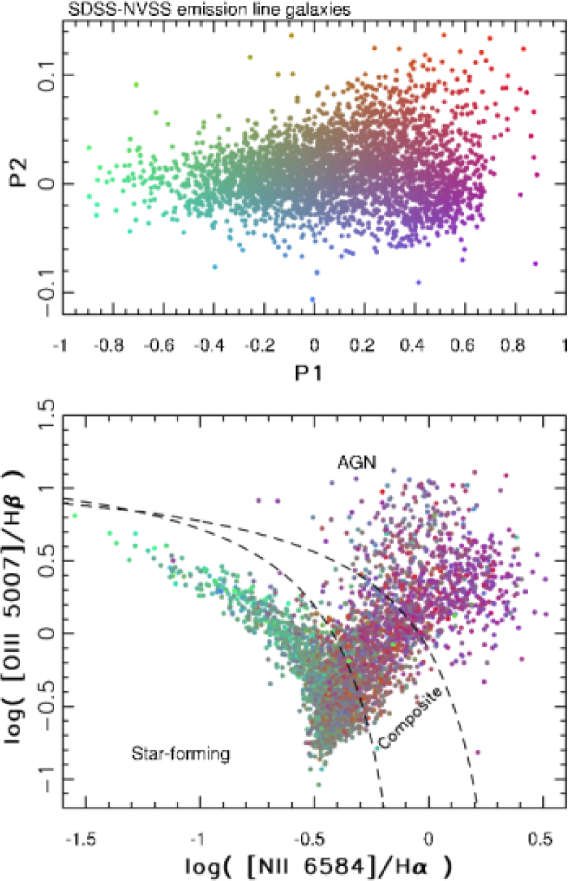
Figure 4.— Top panel: The distribution of $\sim 3,400$ SDSS emission line galaxies, in the redshift range of $0.01$ to $0.3$, drawn from the DR1 “main” spectroscopic sample, which were also detected by the 1.4 GHz NVSS survey, in a diagram constructed with the principal rest-frame colors ($P1$,$P2$). Each dot corresponds to one galaxy, and the color code is determined by the position in this plane. The bottom panel shows the distribution of these galaxies in the (BPT) diagram (Baldwin, Phillips & Terlevich, 1981). The lower dashed line separates the regions populated by star-forming and composite galaxies (Kauffmann et al., 2003). The upper dashed line separates the regions populated by composite and AGN galaxies (Kewley et al., 2001). The dots are colored according to their $P1$ and $P2$ values given in the top panel. Note the strong correlation between the rest-frame colors and the emission line flux ratios (see text for details).

4.1.2 Completeness and contamination due to the photometric selection

In the top panel in Fig. 4 we show the distribution of $\sim 3,400$ SDSS/NVSS emission line galaxies in the ($P1$,$P2$) rest-frame color-color diagram. The color code is determined by the position of a galaxy in this plane. The bottom panel shows the BPT diagram for the same galaxies with the colors adopted from the upper panel. For these radio luminous galaxies, a strong correlation exists between their rest-frame optical colors and emission line properties, in particular between $P1$ and $\log{\left(\mathrm{[NII\,\,6584]/H\alpha}\right)}$. We want to stress that the SDSS/NVSS galaxies with no emission lines in their spectra have typically red $P1$ colors, with a median $P1$ value of 0.46 and an interquartile range of 0.13 (see also e.g. Fig. 12 in Smolčić et al. 2006). This implies that the rest-frame color $P1$ can be used as an efficient separator between AGN and SF galaxies in samples where these two types of galaxies are the two dominant populations.

Smolčić et al. (2006) argued that the $P2$ color is a proxy for the galaxies’ dust content, with higher values of $P2$ corresponding to higher dust attenuation. However, as the dynamic range of $P2$ is very narrow, we will rather base our selection on the $P1$ color alone. Hereafter, based on a compromise between completeness and contamination of the photometrically selected samples of galaxies, we choose a color-cut of $P1$$=$$0.15$ as the dividing photometric value between star forming galaxies ($P1$$\leq$$0.15$) and AGN ($P1$$>$$0.15$). Given this boundary we infer that the sample of photometrically selected star forming galaxies is $85\%$ complete, and contaminated by AGN and composite objects at the $20\%$ and $10\%$ levels, respectively. Vice versa, the photometrically selected sample of AGN is $90\%$ complete and contaminated by SF and composite galaxies at the $5\%$ and $15\%$ level, respectively (see Appendix B.1 for computational details). We will use these estimates in the following analysis to statistically correct the photometrically selected SF and AGN samples in the VLA-COSMOS survey.

4.1.3 Is the rest-frame color based selection method biased against dusty starburst galaxies?

One of the main advantages of radio observations is that the intrinsic physical properties that drive the radio emission can be derived without any need for dust-extinction corrections (as radio emission passes freely through dust). In particular, radio observations provide a dust-unbiased view of star-formation (see Condon 1992 for a review; see also Haarsma et al. 2000). Hence, it is important to address whether our rest-frame color selection technique misses out dusty starburst galaxies. In order to do this we study a sub-sample of SDSS/NVSS galaxies that were also detected with the IRAS satellite at IR wavelengths.

First we address the composition of the ’missed’ $\sim 15\%$ of the SF galaxies (note that the photometrically selected SF galaxy sample is $85\%$ complete) in order to show that our selection does not introduce biases against the most luminous starburst galaxies. About $30\%$ of the SF galaxies with $P1$$>$$0.15$ have IRAS detections, which is consistent with the fraction of IRAS detections in the SF galaxy sample with $P1$$\leq$$0.15$. This suggests that the composition of the missed SF galaxies is not significantly different from the composition of the selected SF galaxies. Second, the fractions of luminous and ultra-luminous IR galaxies (LIRGs and ULIRGs) in the spectroscopically classified SF galaxy samples with $P1$$\leq$$0.15$ and $P1$$>$$0.15$ appear to be consistent with each other. And third, the completeness and contamination of the SDSS/NVSS/IRAS galaxy sub-samples selected using the rest-frame color based classification method is fairly consistent with the properties of the entire SDSS/NVSS sample (see Appendix B.2 for details). All of this implies that the selection criteria for SF and AGN galaxies adopted on the basis of the analysis of the full SDSS/NVSS sample works almost equally efficiently for the IRAS detected sub-sample. Even further, only $\sim 10\%$ and $\sim 5\%$ of star forming LIRGs and ULIRGs galaxies, respectively, are omitted by the method (see Appendix B.2 for details).

It is noteworthy that in the entire SDSS/NVSS/IRAS sample only 48 objects (i.e. $\sim 5\%$) were identified as absorption line AGN, i.e. having no emission lines in their optical spectra. It is possible that very high dust obscuration may suppress the detection of emission lines in the optical spectrum. A visual search for signatures of HII regions in the 48 SDSS color-composite images suggested that at the most $30\%$ of these galaxies may possibly be undergoing star formation (e.g. possible galaxy merger, or extended morphology). Therefore, only a negligible fraction of less than $1.5\%$ of the SDSS/NVSS/IRAS galaxies may be so heavily dust-obscured that no emission lines would be detected in their optical spectra.

In order to test this issue further, we have synthesized the $P1$ color for the ’standard’ dusty starburst galaxies M 82 (a typical LIRG), and Arp 220 (the prototypical ULIRG) using spectral templates given by Polletta et al. (2006). The optical to NIR part of these templates was generated using the stellar population synthesis code GRASIL (Silva et al., 1998). The derived $P1$ colors for M 82 and Arp 220 are 0.078 and 0.149, respectively, implying that M 82 would not have been missed by the rest-frame color based classification method, while Arp 220, although close to the adopted limit in $P1$, still lies within our selection criterion (note that in reality observational photometric errors of M 82- and Arp 220- like objects will introduce a scatter in P1; see also Sec. 4.2.2). Based on the tests presented above we conclude that our rest-frame color based classification method is not significantly biased against dusty starburst galaxies.

4.2. Application of the rest-frame color based classification method to the multi-wavelength photometry of the VLA-COSMOS radio – optical galaxies

In the previous section we have studied, and calibrated, the rest-frame color based classification method using the local galaxy sample. Assuming that evolutionary effects with redshift do not significantly affect the reliability of the classification, we can safely apply it to the galaxies in the VLA-COSMOS 1.4 GHz matched radio sample (Sec. 5.4)   to separate SF from AGN galaxies at intermediate redshifts. However, first we need to derive the rest-frame $P1$ color from the observed SED of the VLA-COSMOS galaxies. We do this via high-resolution SED fitting, described in Sec. 4.2.1, and we test the accuracy of the rest-frame color synthesis in Sec. 4.2.2.

4.2.1 Derivation of rest-frame colors

In order to estimate the rest-frame color $P1$ for each galaxy in the matched radio sample that we do not classify as a star or QSO (see Sec. 5), we use the GOSSIP (Galaxy Observed Simulated SED Interactive Program) software package (Franzetti, 2005), designed for fitting a galaxy’s SED to a set of chosen spectral models. The SED of the galaxies in our sample, that we use for fitting, extends from $3500$ Å to $2.5~{}\mathrm{\mu}$m (comprised in 6 photometric pass-bands) and we fit to each observed SED a realization of $\sim 100,000$ spectra built using the Bruzual & Charlot (2003) stellar synthesis evolutionary models. Star formation histories have been parameterized by an underlying continuous star formation history (decaying exponentially), and randomly superimposed bursts (see also Kauffmann et al. 2003; Kong et al. 2004; Salim et al. 2007). We cover ages between $100$ Myr and $13.5$ Gyr, specific star formation rates (star formation rate per unit galaxy stellar mass) between $10^{-15}$ yr^-1 and $3.93\times 10^{-8}$ yr^-1 and metallicities from a tenth to twice solar.

For each object in our sample the model spectra in our library are redshifted to the galaxy’s measured redshift (spectroscopic where available, otherwise photometric), then each spectrum is convolved with the observed filter response function, and then fitted to the available observed photometric data, using a direct $\chi^{2}$ minimization procedure. Output parameters, such as e.g. rest-frame colors, stellar mass or the 4000 Å break, are taken from the best fit model spectrum. In order to derive physically meaningful output parameters, we restrict the fitting procedure to models that have an age smaller than that of the Universe at the galaxy’s redshift.

4.2.2 Accuracy of the derived rest-frame colors

The synthesized, relative to observed, colors and magnitudes for the VLA-COSMOS galaxies, computed as described above, are reproduced with a satisfying accuracy of $\sim 0.07$ and $\sim 0.04$, respectively. To further test the accuracy of the derived rest-frame color, we synthesize P1 for a sample of $\sim 1700$ local SDSS/NVSS galaxies. For these galaxies the P1 colors, computed from their spectrum (with an accuracy of better than 0.03 magnitudes; see Smolčić et al. 2006), are also available. Thus, comparing $P1$ synthesized via SED fitting with the reference $P1$ derived from the spectrum gives us a direct measure of the achieved accuracy, shown in Fig. 5 (top panel). The root-mean-square-scatter is $\sim 0.1$.

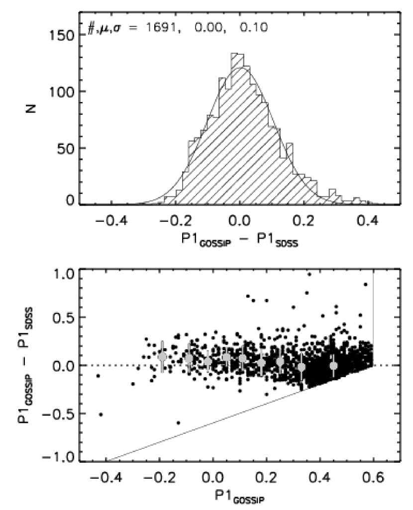
Figure 5.— The comparison of the $P1$ color synthesized from the SDSS spectrum ($\mathrm{P1_{SDSS}}$ that has a typical error of 0.03) and via SED fitting ($\mathrm{P1_{GOSSIP}}$) for $\sim 1700$ SDSS/NVSS galaxies from the DR1 “main” spectroscopic sample (top panel). The $P1$ color is reproduced with a spread of $\sim 0.1$. The bottom panel shows the difference in the $P1$ color as a function of $\mathrm{P1_{GOSSIP}}$. The thin solid lines show the upper $P1$ limits of 0.6, imposed for this analysis. Note the slight systematic trend in the derived $P1$ color as a function of $\mathrm{P1_{GOSSIP}}$ (the large dots are the median offsets, with indicated $1\sigma$ error bars). The trend presumably arises due to the presence of strong emission-lines in the rest-frame wavelength range of $3800-5800$ Å, that are not taken into account in the BC03 models. We use these offsets to correct for these systematics in the derivation of $P1$ for the clean radio sample (see text for details).

In the bottom panel in Fig. 5 we show the difference of the $P1$ color as a function of the synthesized (GOSSIP) $P1$ color for the SDSS/NVSS galaxies. A slight systematic trend is present as a function of the derived $P1$ color. This trend presumably arises from the presence of strong emission lines in the galaxies’ SEDs (in the rest-frame wavelength range that is used to derive $P1$), which are not taken into account in the BC03 model spectra. In our further analysis of the VLA-COSMOS data, we use the median offset, shown in the bottom panel in Fig. 5, to correct the derived $P1$ color, and we consider the synthetic $P1$ color to be accurate to $\sim 0.1$ mag. However, an error of 0.1 mag for 68% of the galaxies, and 0.2 for 95%, may substantially alter the SF/AGN selection, introducing the largest uncertainty for the galaxies that have $P1$ colors close to the chosen $P1$ boundary. To account for these uncertainties, we simulate the $P1$ errors using a randomly drawn Gaussian distribution with a standard deviation of 0.1 centered at zero (see top panel in Fig. 5). These errors are then added to the galaxies’ $P1$ colors derived from the best fit template in the SED fitting, and the SF/AGN selection (see Sec. 5.4) is applied. By repeating this procedure 10,000 times we obtain a robust statistical distribution of the number of selected SF and AGN galaxies yielding $356$ SF and $585$ AGN galaxies (mean) with a root-mean-square scatter of only $7$.

Applying our SF/AGN selection using the P1 distribution obtained from the best fit template in the SED fitting yields 340 SF and 601 AGN galaxies (see Sec. 5.4). Thus, $\sim 5\%$ less SF galaxies are selected. This is easily understood as the blue tail of the $P1$ distribution contains a smaller number of galaxies than there are in the prominent red peak (see e.g. Fig. 24). Therefore, a normal error distribution will systematically scatter more galaxies to the blue $P1$ region, than to the red one. We conclude that the photometric errors of the synthesized $P1$ color introduce a number uncertainty of $\sim 5\%$ in favor of SF galaxies. Although $\sim 5\%$ is not significant, it is necessary to keep this bias in mind in the analysis of the ’population mix’ of submillijansky radio sources (Sec. 7.2).

5. Classification of VLA-COSMOS sources in the matched radio sample

In this section we present the classification of the entire VLA-COSMOS matched radio sample into star candidates (Sec. 5.2), QSOs (Sec. 5.3), SF, AGN and high-z galaxies (Sec. 5.4). We begin with a summary of the sample definitions (Sec. 5.1).

5.1. Outline and nomenclature

In Sec. 4.1 (see also Appendix B) we have presented the calibration and effectiveness of the rest-frame color based classification method for separating galaxies dominated by star formation from those dominated by AGN activity. For this we have used the SDSS “main” spectroscopic sample – a pure galaxy sample that by definition does not contain any star-like objects (Strauss et al., 2002). This, obviously, implies that the same effectiveness of the method can only be reached if the rest-frame color based classification method is applied to a comparable sample, i.e. galaxies only. However, our VLA-COSMOS matched radio sample consists not only of galaxies, but also of stellar like sources, where the latter are either stars or quasi stellar objects (QSOs). Therefore, we classify the sources in the matched radio sample into five sub-types – a) star candidates, b) quasi stellar objects (QSOs), c) active galactic nuclei (AGN), d) star forming (SF), and e) high redshift ($z>1.3$; high-z) galaxies. The latter three sub-types compose our “VLA-COSMOS galaxy sample”. The properties of each sub-type are summarized as follows.

• Stars: Point-sources in the optical, with their SEDs best fit using a stellar template.

• OSQs: Point-sources in the optical (stellar-like SEDs are excluded; see above). This criterion essentially requires that the emission of the nucleus in the optical strongly dominates over the emission of the host galaxy. Thus, this sample predominantly contains broad line AGN (i.e. type-1 AGN), with power law spectra in the optical.

• AGN: Galaxies (not point-sources) whose rest-frame color properties are consistent with properties of AGN ($P1$ $>$ $0.15$, X-ray luminosity above $10^{42}$ erg s^-1 if X-ray detected). This selection requires that the optical emission either shows signs of both, the emission from the central AGN as well as the emission from the underlying host galaxy, or only the latter. Thus, this sample essentially includes Seyfert and LINER types of galaxies, as well as absorption line AGN, and we limit it to redshifts of $z\leq 1.3$.

• SF galaxies: Galaxies whose rest-frame color properties are consistent with properties of star forming galaxies ($P1$ $\leq$ $0.15$). Thus, the emission of these galaxies is dominated by the emission originating from regions of substantial star formation. This sample is also limited to redshifts $\leq 1.3$.

• high-z galaxies: Galaxies (not point-sources) with redshifts beyond $z=1.3$.

5.2. Star candidates

In order to identify star candidates in the VLA-COSMOS matched radio source sample, we make use of the COSMOS stellar catalog (Tasca et al., 2007), that was constructed from the HST/ACS catalog (Leauthaud et al., 2007) using stellar templates to fit the entire SED of each source. In Fig. 6 we show the color-color distribution for $\sim 2,000$ objects in the COSMOS field securely classified as stars (with photometric errors better than 0.05), which form well defined loci in the broad-band color-color diagrams. Cross-correlating our matched radio sample with the COSMOS stellar catalog yields only 2 objects detected in the radio regime that are consistent with having stellar properties. The color properties of these objects are shown in Fig. 6. Within the error-bars they are consistent with the main stellar loci. Note, however, the $r^{+}$-$i^{+}$ color excess of one of the star candidates in the $r^{+}$-$i^{+}$ vs. $g^{+}$-$r^{+}$ color-color diagram (middle panel in Fig. 6), which suggests consistency with properties of e.g. cataclysmic variables (e.g. Szkody et al. 2002, 2003), or unresolved binary star systems containing a white dwarf and a late type star (e.g. Smolčić et al. 2004). The best fit stellar templates for these objects were taken from the PHOENIX library (Hauschildt et al., 1997) and represent dwarfs with effective temperatures in the range of 4100 to 5000 K and $\log{(g)}$ in the range of 3 to 3.5. The 1.4 GHz total flux densities for these two objects are 126 and 152 $\mathrm{\mu}$Jy, and the corresponding $i$ band AB magnitudes are 25.34 and 23.28, respectively. It is noteworthy that both objects have IRAC counterparts, but no associated X-ray emission. We consider these two sources to be star candidates, however a more detailed analysis (using for example spectroscopy), which is beyond the scope of this paper, would be needed to verify this. Such a low fraction of identified stars is consistent with star detection rates in other deep radio surveys (e.g. Fomalont et al. 2006).

The two star candidates in our radio sample form only $\sim 0.1\%$ of the VLA-COSMOS radio sources, and we exclude them from our sample for further analysis.

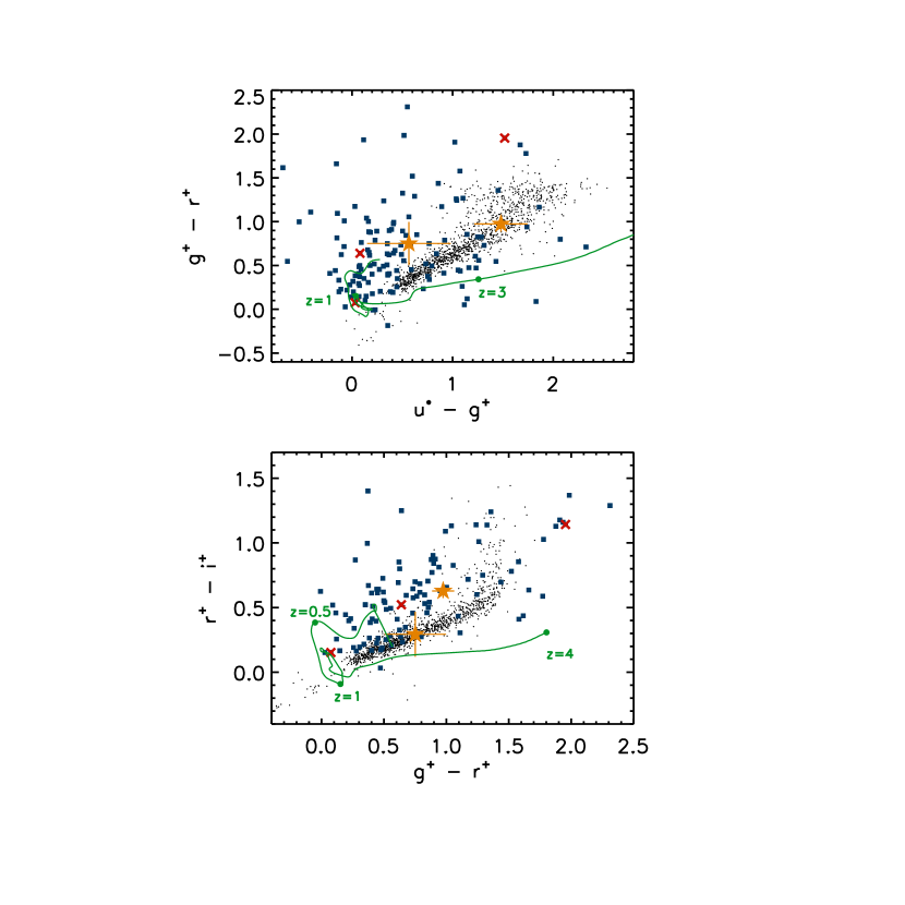
Figure 6.— Color-color diagrams for COSMOS stars and VLA-COSMOS QSOs (see text for details). The stars (black dots) form a narrow, well defined, locus in each diagram. The star symbols (yellow) show 2 objects detected in the VLA-COSMOS radio survey, identified as star candidates (see text for details). VLA-COSMOS objects classified as QSOs by our selection criteria (blue squares) are also shown, and they occupy the ’standard’ QSO regions in these diagrams (see text for details). The crosses (red) show objects classified as a QSO by our technique, yet their spectra were identified as red galaxies. QSO evolutionary tracks are shown to guide the eye (green curved lines).

5.3. Quasi stellar objects

5.3.1 Identification based on morphology

In order to identify QSOs in our matched radio sample we rely on an optical classification, rather than using X-ray emission, due to the much higher sensitivity of the observations in the optical ($5\sigma$ sensitivity limit in the Subaru $i$ band is 26.2; see Capak et al. 2007). For example, if one would select AGN relying purely on e.g. X-ray – to – optical flux ratios, which are generally greater than 0.1 for both broad and narrow line AGN (e.g. Maccacaro et al. 1988; Alexander et al. 2001), with our optical limit of $i=26$ (corresponding to $r^{+}$ of $\sim 27$) the depth of the X-ray point-source detection would have to be about 2 orders of magnitude deeper than it currently is in order to select a complete sample of AGN. Further, a clear distinction between broad and narrow line AGN would not be possible. Hence, here we identify a QSO by requiring that a given source in the matched radio sample is optically compact. In Fig. 7 we show the fitted $i$ band FWHM of the sources in the COSMOS photometric catalog (Capak et al., 2007) as a function of their $i$ band magnitude. Point-sources (black squares), selected from the HST/ACS catalog (Leauthaud et al., 2007), form a locus in this plane, separated from the area occupied by extended sources. However, the point-source locus is fairly scattered, especially at faint magnitudes, and thus makes a single automatic cut at a certain FWHM value inefficient. For this reason, we classify sources within the FWHM range of $1.85^{\prime\prime}-2.05^{\prime\prime}$ as QSOs only if their optical HST morphology was visually confirmed to be ’point-source dominated’. However, we consider all sources below FWHM of $1.85^{\prime\prime}$ to be QSOs. We further supplement this sample with 12 objects that were classified as point-sources in the HST/ACS catalog, but do not satisfy the above criteria.

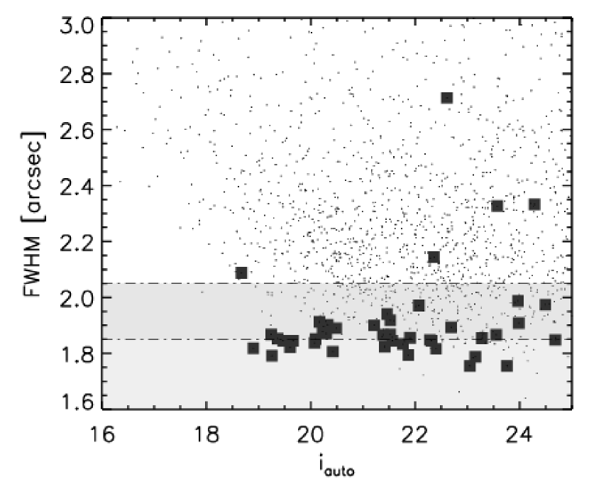
Figure 7.— FWHM of the optical counterparts of the matched radio sources (small dots) as a function of $i$ band magnitude, taken from the COSMOS photometric catalog (Capak et al., 2007). Grey squares represent the HST/ACS point sources in the sample. Unresolved sources form a separated locus in this diagram. We identify QSOs by requiring that a source is optically compact by choosing an absolute separation value of $\mathrm{FWHM}\lesssim 1.85^{\prime\prime}$ (below lower dash-dotted line; light-grey shaded area). In the range of FWHM $\in(1.85,2.05]^{\prime\prime}$ (between upper and lower dash-dotted lines; dark-grey shaded area) we identify objects as QSOs only if they were visually confirmed to be point-source dominated (see text for details).

In summary, out of 1558 objects we identify 139 (i.e. $11.5\%$) as QSOs. In Fig. 6 we show their broad-band ($u^{*}$,$g^{+}$,$r^{+}$,$i^{+}$) color-color properties. As expected, the non-stellar emission of the selected objects confines them to regions typical for QSOs, which are separated from the main stellar loci in these diagrams (e.g. Brusa et al. 2007a; Richards et al. 2002). A minor fraction of these objects lie on the stellar loci. However, in the $BzK$ diagnostic diagram, which is an efficient tracer for stars (Daddi et al., 2004) these sources are offset from the stellar locus, verifying their non-stellar nature.

As AGN dominated systems usually have soft X-ray to optical flux ratios in the range of about $0.1$ to $10$ (e.g. Maccacaro et al. 1988; Alexander et al. 2001), we can use the X-ray to optical flux properties of the identified QSOs to further test our selection criteria. 43 objects in our QSO sample were detected as X-ray point-sources, and their X-ray to optical flux ratios are consistent with the expected values. The median $r^{+}$ magnitude for these sources is 21.3. For the remaining QSO candidates, that were not detected in the X-rays, the median $r^{+}$ is 24.4. Therefore, these sources are also consistent with the expected X-ray to optical flux ratios, however beyond our X-ray point-source detection limit ($10^{-15}$ erg cm^-2 s^-1 in the soft band). We conclude that the independent analysis of the X-ray properties of our selected QSOs verifies the validity of our selection.

5.3.2 Spectroscopic verification

A sub-sample of 31 objects of the 139 previously identified QSOs have available optical spectroscopy with secure classifications (Trump et al., 2007; Prescott et al., 2006; Colless et al., 2001; Schneider et al., 2005), and only 3 of these objects were classified as red galaxies (Trump et al., 2007), while all the others have AGN classifications. The 3 galaxies classified as ellipticals were identified as QSO candidates by our method based on visual/morphologic classification, which suggests the presence of dominating nuclear emission. The color properties of two of theses objects (see red crosses in the top panel in Fig. 6) are also consistent with the color properties of quasars. Thus, we conclude that the selected QSO sample is not significantly ($\lesssim 10\%$) affected by contamination of non-QSO objects.

In order to assess the completeness of the selected QSO sample, we search for objects that are spectroscopically classified as QSOs and ’missed’ by our classification method. Our criteria yielded 139 objects classified as QSOs in the matched radio sample, and in the remainder of the sample (i.e. the 1417 sources that were not classified as star candidates or QSOs) spectroscopic classifications are available for 397 objects. Out of these, 9 were spectroscopically classified as QSOs. Two SDSS examples, for which COSMOS HST/ACS imaging is available, are shown in Fig. 8. They obviously show extended optical emission, and a substantial light component arises from the host galaxy itself. The median redshift of these 9 objects is only 0.4. It is noteworthy that all of these objects have X-ray point source detections, and all except one have X-ray luminosities higher than $10^{42}$ erg s^-1. Therefore these galaxies will be selected into our AGN class, hence not contaminating the SF galaxy sample (see Sec. 5.4). As the spectroscopic sub-sample fairly represents the full matched radio sample (see Fig. 3), we conclude, based on the above analysis, that the sample of identified QSOs is about 80% complete. As expected, the incompleteness is mostly due to relatively low redshift, low-luminosity AGN.

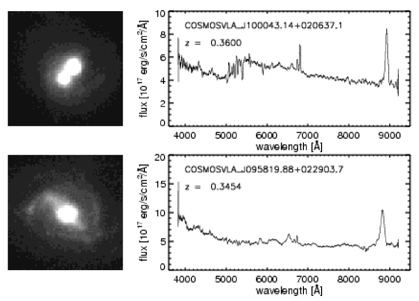
Figure 8.— HST/ACS stamps ($4^{\prime\prime}$ on the side; left panels) and the corresponding SDSS spectra (smoothed using $20$ Å wide bins; right panels) for two sources that were spectroscopically classified as QSOs, but missed by our QSO selection method. The morphology of these sources is clearly extended (in particular the source in the top panel is possibly a merging system with double nuclei visible, and extending beyond the displayed $4^{\prime\prime}$).

5.4. Star forming and AGN galaxies

In the previous sections we have identified 2 star candidates and 139 QSOs in the matched radio sample. We will refer to the 1417 remaining sources in the matched radio source sample as the ’galaxy sample’. Before applying the rest-frame color based classification method to our VLA-COSMOS galaxies in order to separate SF from AGN galaxies, we restrict the galaxy sample to 941 galaxies with redshifts $\leq 1.3$, as a) the photometric redshifts are less reliable beyond this redshift, and b) the library of BC03 model spectra that we use for the SED fitting may not be appropriate for fits beyond this redshift as the distribution of priors was set to optimally match this intermediate redshift range. Hereafter, we will call the sample of 476 galaxies with redshifts greater than 1.3 high redshift (high-z) galaxies.

We perform an SED fit using GOSSIP (as described in Sec. 4.2) for each of the 941 objects in the matched radio ’galaxy’ sample out to $z=1.3$. The distribution of the rest-frame color $P1$ for these galaxies is shown in Fig. 9. The distribution is very similar to that of the local sample (see top panel in Fig. 24) with a peak at $P1$$\sim 0.4$ (AGN) and a prominent tail towards bluer values (SF galaxies). We inspected the behavior of the median value of the synthesized $P1$ color for the entire $z\leq 1.3$ galaxy sample as a function of redshift, and we found no significant evolution in the median color. We reached the same conclusion analyzing the median $P1$ colors of the SF and AGN sub-populations. This implies that a fixed cut in the color can safely be applied to the entire galaxy population out to $z=1.3$.

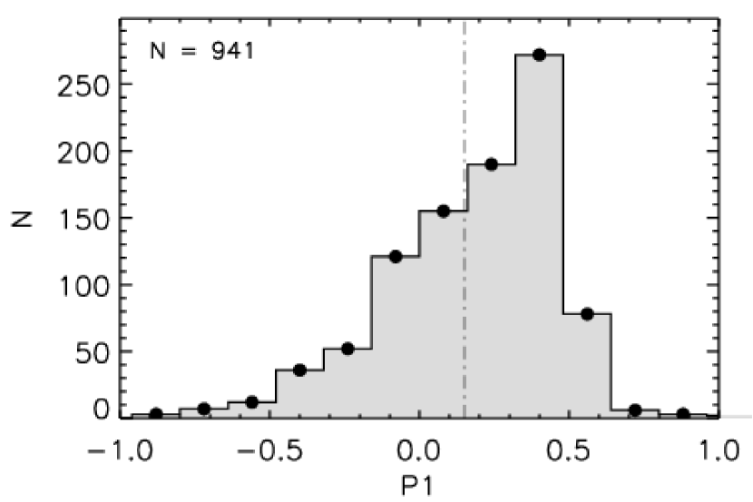
Figure 9.— The distribution of the synthesized rest-frame $P1$ color, corrected for the systematics (see bottom panel in Fig. 5), for the objects in the matched radio galaxy sample with $z\leq 1.3$. Note, that the expected distribution from our local sample, showing a prominent tail towards bluer values of $P1$, is reproduced. The dash-dotted line indicates our chosen boundary for separating star forming from AGN galaxies.

The SED fitting was performed via a $\chi^{2}$ minimization procedure. The median value of the reduced $\chi^{2}$ of the SED fits, computed using the best fit model spectrum, is $0.6$ with an interquartile range of $2$. Only 10% of the fitted objects have reduced $\chi^{2}$ values above 5, and only 5% above 10. A visual inspection suggests that these galaxies are either nearby galaxies, which are resolved and often saturated in the Subaru $i$ band, or QSO contaminants. While the latter predominantly have blue $P1$ colors, the synthesized $P1$ color for the first class of galaxies still appears to be a valid tracer for the SF/AGN separation, and therefore we do not reject them from the sample. In order to select SF and AGN galaxies we require that the synthesized $P1$ color is $\leq$ $0.15$ and $>$ $0.15$, respectively. However, to improve our selection at this point we make use of the X-ray properties in the soft band of the 114 galaxies that were detected as X-ray point sources. Namely, if the soft X-ray luminosity of an object is greater than $10^{42}$ erg s^-1 we consider it to be an AGN, regardless of its $P1$ color. Note that this criterion is expected to reduce the contamination of the SF sample by objects with blue rest-frame colors, such as QSOs missed by our selection. Out of the 114 X-ray detected sources, 77 have X-ray luminosities greater than the above given value, and 37 out of these 77 have a synthetic $P1$ color $\leq$ $0.15$. In summary, our selection yields 340 SF and 601 AGN galaxies in our matched radio galaxy sample with $z\leq 1.3$. We analyze these galaxies further in Sec. 7.

6. Comparison with other selection methods

In this Section we compare our classification method, that we have applied to an intermediate redshift population, with other classification methods used for both local and intermediate redshift populations in the literature (Lacy et al., 2004; Stern et al., 2005; Best et al., 2005a). We also study the 24$\mathrm{\mu}$m properties of our radio sources, and their correlation to the 1.4 GHz emission.

6.1. 3.6-8 $\mathrm{\mu}$m color – color diagnostics

QSOs, whose UV to NIR continuum is dominated by a power law, tend to be redder than other types of galaxies in the MIR. Hence, they occupy a distinct region in MIR color space, and several color-color criteria were suggested for their selection (Lacy et al., 2004; Stern et al., 2005). In Fig. 10 we compare our classification method with those proposed in the MIR using a sub-sample of the matched radio sources that were also detected with IRAC ($\sim 90\%$ have IRAC counterparts; see Sec. 3.2). We indicate the QSO (dots), AGN (thin contours) and star forming (thick contours) galaxies selected using our method. The dashed lines in the top and bottom panel in Fig. 10 show the color-color criteria proposed by Lacy et al. (2004) and Stern et al. (2005), respectively, for the selection of broad-line AGN. As expected, the majority of objects selected as QSOs by our method falls within this region, reassuring the efficiency of the classification method presented here. There are several QSO candidates outside these regions, which is not surprising as the suggested ’quasar regions’ do not select a 100% complete sample of QSOs, and a certain amount of outliers is expected (see Stern et al. 2005 for a discussion of this point). In Sec. 5.3 we have inferred that our selected sample of QSOs is not significantly contaminated by different types of objects, which is affirmed by this independent analysis.

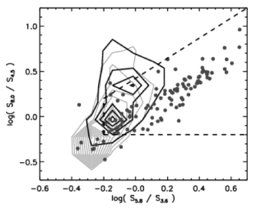
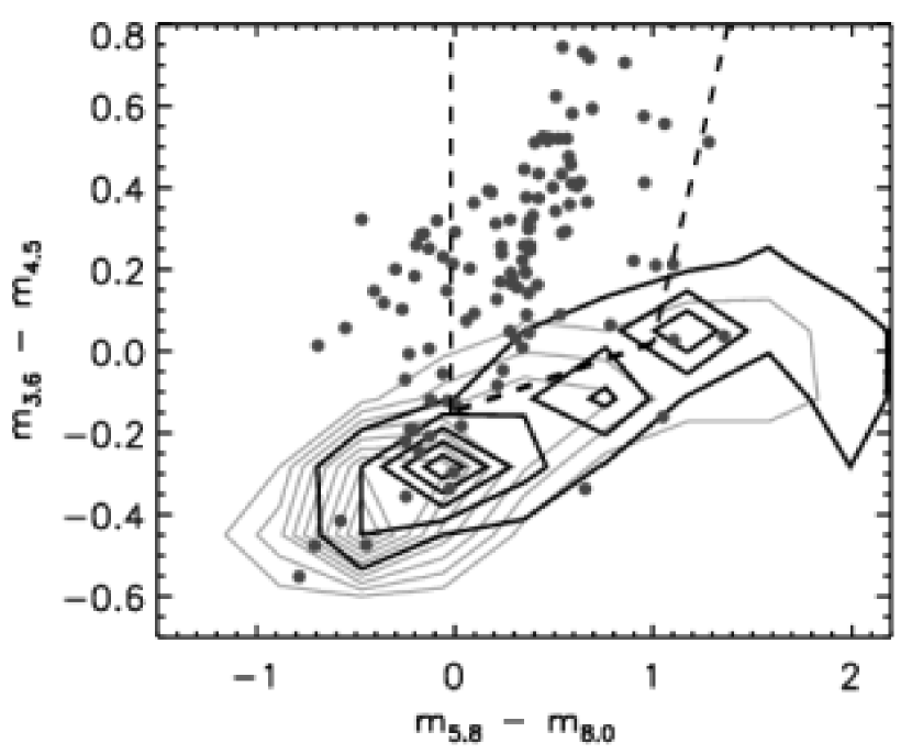
Figure 10.— IRAC color-color diagrams in two representations (top and bottom panel) used as diagnostic tools for the separation of QSOs (broad line AGN) from ’normal’ galaxies (Lacy et al., 2004; Stern et al., 2005). Filled circles display the 122 QSOs selected by our morphologic method that have IRAC detections; thin and thick contours show the 579 AGN and 322 star forming galaxies separated by our rest-frame color based classification method, respectively, that have IRAC counterparts. The contour levels in both panels are in steps of 7 starting at 7. The dashed lines in the top and bottom panels show the empirically selected regions for identifying broad-line AGN proposed by Lacy et al. (2004, top panel) and Stern et al. (2005, bottom panel), respectively.

Stern et al. (2005) showed that at redshifts of $\lesssim 1$ galaxies span a large range in the $m_{5.8}-m_{8.0}$ color, which is consistent with the horizontal extent of our selected star forming and AGN galaxies (see bottom panel in Fig. 10). However, typical low luminosity AGN and starburst galaxies cannot be clearly divided using these diagnostic diagrams (see also color evolutionary tracks in Fig. 19). Nonetheless, elliptical galaxies (which correspond to our class of absorption line AGN) tend to occupy the bottom left regions in both diagrams, and close to these regions the distributions of our identified AGNs peak. On the other hand, the peak of the distribution of our selected star forming galaxies in these diagrams is clearly displaced from the one for AGN. We would like to stress that this independently confirms that indeed two different populations of galaxies have been selected. The differences in the MIR properties of our SF and AGN galaxies affirm the strength of the rest-frame color based classification method.

Further, Stern et al. (2005) showed that narrow line AGN appear spread out in both the QSO and galaxy regions, which is also a result of our selection method [note that the selected AGN are present in both regions]. The last point we want to stress is that the star forming galaxy locus in these diagrams is also consistent with the expected colors, as a ’contamination’ by star forming galaxies of the QSO locus is expected, especially close to the boundary. In summary, the classification method presented here agrees remarkably well with the expected properties of QSOs, AGN and star forming galaxies at intermediate redshifts in the MIR range encompassing 3.6-8 $\mathrm{\mu}$m.

6.2. 24 $\mathrm{\mu}$m properties: The 24 $\mathrm{\mu}$m – radio correlation

A tight mid-IR (as well as far- and total- IR) – radio correlation is expected for star forming galaxies, while ’radio-loud’ AGN are expected to strongly deviate from it (e.g. Condon 1992; Bell 2003; Appleton et al. 2004). The 60 $\mathrm{\mu}$m – radio correlation for low-luminosity AGN was studied by Obrić et al. (2006) in the local universe. Based on a selection utilizing the BPT diagram they have shown that also low -luminosity AGN follow a tight FIR – radio correlation, however with a slightly different slope and a larger scatter than SF galaxies. In this section we investigate the 24 $\mathrm{\mu}$m – radio correlation for our selected SF and AGN galaxies. In particular, if our SF/AGN separation method is successful, then a difference in the 24 $\mathrm{\mu}$m compared to 20 cm properties is expected to be seen for the two populations.

Our rest-frame color based classification method has identified 340 SF galaxies. Out of these $82\%$ (280) were detected at 24 $\mathrm{\mu}$m with a signal to noise $\geq 3$. On the other hand, out of 601 selected AGN only $44\%$ (267) have a MIPS 24 $\mathrm{\mu}$m detection with $\mathrm{S/N}\geq 3$. In Fig. 11 we show the 24 $\mathrm{\mu}$m vs. 1.4 GHz luminosity (top panel) for our SF and AGN galaxies, where the 24 $\mathrm{\mu}$m data was not k-corrected. A correlation between the two luminosities exists for both types of objects detected at 24 $\mathrm{\mu}$m, although on average for a given $\mathrm{L_{\mathrm{1.4GHz}}}$ the 24 $\mathrm{\mu}$m luminosity is slightly lower for AGN than for SF galaxies (see also below). For the SF and AGN galaxies that were not detected at 24 $\mathrm{\mu}$m we have computed upper limits of the 24 $\mathrm{\mu}$m luminosity using the detection limit of the S-COSMOS MIPS shallow survey which is 0.3 mJy. These limiting luminosities are also shown in Fig. 11. Note that for AGN galaxies, as $56\%$ of them are not detected at 24 $\mathrm{\mu}$m, the scatter in the correlation is significantly increased by these objects.

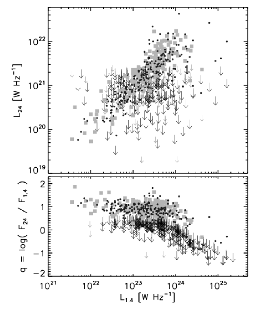
Figure 11.— Top panel: 24 $\mathrm{\mu}$m luminosity vs. 1.4 GHz luminosity for our selected SF (grey squares) and AGN (black dots) galaxies. Upper 24 $\mathrm{\mu}$m luminosity limits for the radio SF ($18\%$) and AGN ($56\%$) galaxies that were not detected at 24$\mathrm{\mu}$m are indicated by grey and black arrows, respectively. Bottom panel: The $q$ parameter, defined as the logarithm of the 24 $\mathrm{\mu}$m to 20 cm flux ratio, as a function of 20 cm luminosity for SF (grey squares) and AGN (black dots) galaxies. Upper limits are indicated by arrows, as in the top panel. Note the much larger scatter in $q$ for AGN than for SF galaxies.

To quantify the correlation, we derive the classical $q$ parameter (e.g. Condon 1992) as the logarithm of the 24 $\mathrm{\mu}$m to 1.4 GHz observed flux ratios. This parameter essentially measures the slope of the correlation, and in the bottom panel in Fig. 11 we show it as a function of $\mathrm{L_{\mathrm{1.4GHz}}}$ for our SF and AGN galaxies, with indicated upper limits (derived as described above). The $q$ parameter seems to show a decreasing trend with increasing radio luminosity. However, this trend is dominated by the objects that have only estimated upper limits, and therefore may be mimicked by the flux limits of the samples. A more detailed analysis of this issue is beyond the scope of this paper.

Figure 12.— The distribution of the $q$ parameter (see also Fig. 11) for SF (top panel) and AGN (bottom panel) galaxies. In both panels the solid histograms show the distribution of the 1.4 GHz sources detected at 24 $\mathrm{\mu}$m  while the dash-dotted histograms represent the distribution of the upper limits of $q$ obtained for the radio sources that were not detected at 24 $\mathrm{\mu}$m (see text for details). The solid vertical line in each panel designates the median value of the entire distribution, also listed in the top left in each panel.

The distribution of the $q$ parameter for SF and AGN galaxies is shown in Fig. 12, for galaxies detected at 24 $\mathrm{\mu}$m and those which only have upper limits. The median $q$ value for SF galaxies is $0.82\pm 0.05$ with a scatter of $\sim 0.3$ when all objects (also the upper limits) are taken into account. On the other hand, the median $q$ value for the AGN galaxies is $0.51\pm 0.02$, significantly lower than for SF galaxies. We also find a larger spread in q ($\sim 0.4$) for the AGN population. Note, however, that the spread quoted here should be considered somehow tentative, especially for AGN, as the exact $q$ values for the fraction of objects not detected at 24 $\mathrm{\mu}$m are not known. Nonetheless, this does not affect the estimates of the median values. Our $q$ parameter derived for SF galaxies is remarkably consistent with the one inferred by Appleton et al. (2004) at 24 $\mathrm{\mu}$m. Combining Spitzer – MIPS and VLA observations in the First Look Survey with optical spectroscopy, they have found a $q$ value of 0.84 with a spread of 0.28 (with no k-corrections applied). They have also shown that the FIR luminosities of AGN tend to be lower for a given radio luminosity, consistent with our findings here.

Finally, in Fig. 13 we show the $q$ parameter as a function of redshift for our SF and AGN galaxies. $q$ does not depend on redshift, both for SF and AGN galaxies, implying that the MIR – radio correlation with the same slope is valid out to high redshifts ($z\sim 1.3$). This result is again consistent with those presented in Appleton et al. (2004).

In summary, the above results have shown that the 24 $\mathrm{\mu}$m – radio correlation has different properties for our selected SF and AGN galaxies, which verifies the efficiency of our rest-frame color based classification method.

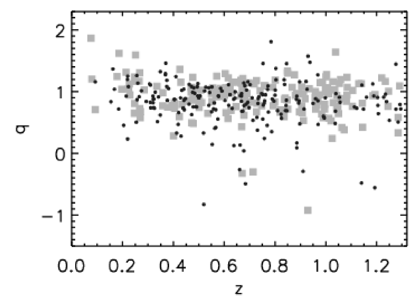
Figure 13.— $q$ as a function of redshift for SF (grey squares) and AGN (black dots) galaxies. Note that $q$ does not depend on redshift, implying that the 24 $\mathrm{\mu}$m– radio correlation holds out to high redshift (see text for details).

6.3. Selection based on optical spectroscopic properties, radio luminosity and stellar mass

Best et al. (2005a) defined a sample of $\sim 3000$ local ($0.01<z<0.3$) galaxies from the SDSS DR2 “main” spectroscopic sample matched with sources above 5 mJy detected in the NVSS survey. They further divided the radio – optical source sample into AGN and SF galaxies making use of the galaxies’ location in the plane spanned by the $4000$ Å break [$\mathrm{D}_{\mathrm{n}}(4000)$] and radio luminosity [$\mathrm{L}_{1.4\mathrm{GHz}}$] normalized by stellar mass [$\mathrm{M}_{*}$]. In Fig. 14 we compare our rest-frame color based classification method with the one utilized by Best et al. (2005a) in the local universe. The $\mathrm{D}_{\mathrm{n}}(4000)$ vs. $\log{\left(\mathrm{L}_{1.4\mathrm{GHz}}/\mathrm{M}_{*}\right)}$ distribution for all galaxies in the matched radio source sample is shown in Fig. 14. The 1.4 GHz luminosity for these galaxies was derived, and $\mathrm{D}_{\mathrm{n}}(4000)$ and $\mathrm{M}_{*}$ from the best fit template from the SED fitting (see Sec. 4.2.1). The average errors are indicated. The dashed line corresponds to the separation between SF and AGN proposed by Best et al. (2005a), and the two types of symbols designate the SF (squares) and AGN (dots) galaxies identified by our rest-frame color based classification method. We want to note that Best et al. calibrated their separation method using a slightly different selection of objects in the BPT diagram (see their Fig. 9) with respect to the one we use here. Therefore, a perfect correspondence between our and the Best et al. method is not to be expected, even if our derived quantities were absolutely accurate. The area in the $\mathrm{D}_{\mathrm{n}}(4000)$ vs. $\log{\left(\mathrm{L}_{1.4\mathrm{GHz}}/\mathrm{M}_{*}\right)}$ plane where the major disagreement is expected, due to the different selections in the BPT diagram, is in the range of $1.4<$$\mathrm{D}_{\mathrm{n}}(4000)$ $<1.6$, and $11<\log{\left(\mathrm{L}_{1.4\mathrm{GHz}}/\mathrm{M}_{*}\right)}<12$. This is the region where a larger fraction of Seyfert and LINER galaxies is located (see Fig. 9 in Best et al. 2005a), and, different from Best et al., we define these galaxies exclusively as AGN. In this region in Fig. 14 we indeed see the largest disagreement between the two classifications. Further, the existence of objects with $\mathrm{D}_{\mathrm{n}}(4000)$ $<1.3$ that we classify as AGN is not surprising, but it rather reflects the dual properties of composite objects, which in this case were classified as AGN by our rest-frame color based classification method. We also want to note that the average error in the synthesized $\mathrm{D}_{\mathrm{n}}(4000)$ [derived from comparison with the spectroscopic and synthetic $\mathrm{D}_{\mathrm{n}}(4000)$ in the local sample] is fairly large, and thus prevents a more detailed comparison between the two selection methods. Overall, given the error bars and the difference in the basic selections of the two methods, as well as the fact that our $\mathrm{D}_{\mathrm{n}}(4000)$ values are not spectral measurements on the data, but values taken from the best fit template, we conclude that our rest-frame color based classification method agrees well with the one proposed by Best et al. (2005a) in the local universe.

In summary, our rest-frame color based classification method for separating SF from AGN galaxies agrees well with other selection schemes, proposed in the literature, which are based both on MIR colors and optical spectroscopic diagnostics.

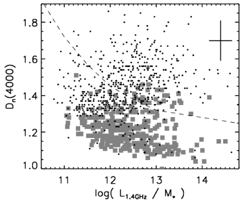
Figure 14.— The $4000$ Å break, $\mathrm{D}_{\mathrm{n}}(4000)$, vs. 1.4 GHz radio luminosity normalized by stellar mass, $\mathrm{L}_{\mathrm{1.4GHz}}/\mathrm{M}_{*}$ for galaxies in the matched radio sample. $\mathrm{M}^{*}$ and $\mathrm{D}_{\mathrm{n}}(4000)$ were synthesized via SED fitting by GOSSIP. The black and grey symbols show objects classified by our rest-frame color based classification method as AGN and star forming galaxies, respectively. The dashed line corresponds to the separation proposed by Best et al. (2005a) for local galaxies. The average errors of the synthesized quantities are shown in the top right. A good consistency between the two selection methods exists, given the large error bars, as well as a slightly different selection rational used here and in Best et al. (2005a; see text for details).

7. Discussion: The composition of the faint radio population

In previous Sections we have presented, tested, and discussed in detail the photometric classification method which we used to separate the matched radio source sample into stars, QSOs, star forming, AGN and high-z galaxies. In this Section we discuss the properties of the ’population mix’ in the VLA-COSMOS survey: In Sec. 7.1 we describe the redshift and luminosity distributions of the selected SF and AGN galaxies, and in Sec. 7.2 we study the contribution of different source types to the sub-mJy radio population. We show, based on the matched radio sample, as well as on the remaining radio sources with no optical counterparts (brighter than $i=26$), that star forming galaxies do not dominate the sub-mJy sources, but that the majority of these sources is rather comprised of AGN and QSOs.

7.1. The redshifts and luminosity distributions of SF and AGN galaxies out to $z=1.3$

The rest-frame color based classification method yielded 340 star forming and 601 AGN galaxies out to redshifts of $1.3$. In the top panel in Fig. 15 we show the redshift distribution for these galaxies using redshift bins of 0.217 in width. We use such wide redshift bins to assess the average properties of the radio population, reducing the effects of fluctuations due to the strong and narrow overdensities which are known to exist in the COSMOS field (Scoville et al., 2007a; Finoguenov et al., 2007; Smolčić et al., 2007b). Poisson errors are indicated for each bin. The deficit of galaxies at the low-redshift end reflects the relatively small comoving volume sampled by the 2$\Box^{\circ}$ area of the COSMOS field at these redshifts. The decline in the number of sources at the high-redshift end, on the other hand, reflects the detection limit of the VLA-COSMOS survey. The redshift distribution of the number of star forming galaxies seems to be more uniform than the one for AGN, in particular the relative number of star forming galaxies compared to AGN rises at higher redshifts ($z\sim 1$). This may be explained by the relatively high number density of ULIRGs expected at these redshifts (Le Floc’h et al., 2005; Caputi et al., 2007) in conjunction with the VLA-COSMOS detection limit which at these redshifts allows to sample only radio luminosities larger than $3\times 10^{23}$ WHz^-1 (see Fig. 16 below). Further, as the comoving volume surveyed at $z\sim 1$ is larger than the one surveyed locally, the probability of detecting a ULIRG is also increasing at these redshifts. Effects of cosmic variance as a function of redshift cannot be excluded, however they should be smaller than for other deep radio surveys that typically probe significantly smaller areas. An increase of the AGN fraction at $z\sim 0.7$ is discernible. It possibly arises due to the dense large scale structure component in the COSMOS field at this redshift (Scoville et al., 2007b; Guzzo et al., 2007).

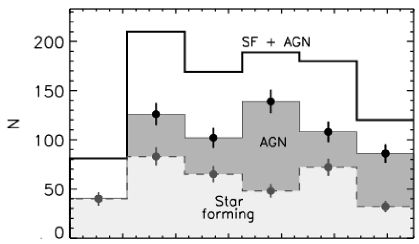
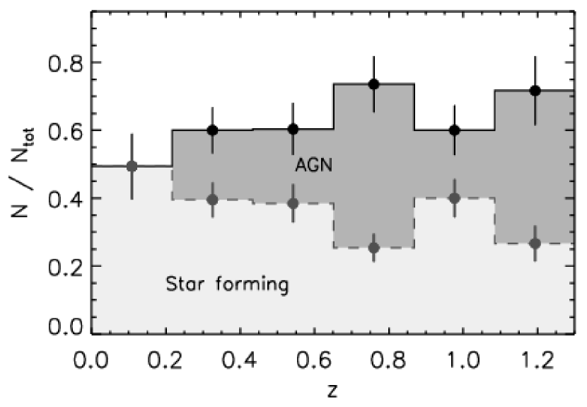
Figure 15.— Top: Redshift distribution of i) the galaxies in the matched radio sample out to $z=1.3$ (thick line), ii) the 340 selected star forming galaxies (light-grey shaded histogram) and iii) 601 identified AGN (dark-grey shaded histogram). Bottom: The fractional distribution of the SF and AGN galaxies compared to the total number of galaxies in the matched radio sample out to $z=1.3$ as a function of redshift. In both panels Poisson errors are indicated.

In the bottom panel in Fig. 15 we show the fractional contribution of the SF and AGN galaxies to the $z\leq 1.3$ matched radio population, as a function of redshift. On average, we find that the mean fractional contribution of SF and AGN galaxies to the $z\leq 1.3$ matched radio population is $(34\pm 14)\%$ and $(66\pm 14)\%$, respectively. This is strikingly similar to the relative numbers of SF and AGN galaxies in the local Universe. Namely, if we apply the adopted $P1$ color cut to the SDSS/NVSS galaxy sample (see Sec. 4.1), we find that $\sim 32\%$ of the galaxies are star forming, and $\sim 68\%$ are AGN. If, as shown by the tests described in Sec. 4.1, our rest-frame color based classification method can reliably be applied also to high redshift galaxies, then the similarity of the SF and AGN fractions suggests that the two populations have similar evolutionary properties out to $z\sim 1.3$.

In Fig. 16, we show the 1.4 GHz luminosity as a function of redshift for the selected SF and AGN galaxies out to $z=1.3$. We also indicate the expected luminosity ranges for Milky Way type galaxies, LIRGs, ULIRGs and HyLIRGs, which were derived using the total IR – radio correlation (Bell, 2003). It is noteworthy that the majority of galaxies with luminosities typical for HyLIRGs ($\mathrm{L_{IR}}>10^{13}$ $\mathrm{L}_{\odot}$) was classified by the rest-frame color based classification method as AGN, consistent with the expected properties of these galaxies (e.g. Veilleux et al. 1999; Tran et al. 2001). This point is seen more clearly in Fig. 17, where we show the distribution of the 1.4 GHz luminosity for the selected star forming and AGN galaxies. The median luminosities are $\sim 1.6\times 10^{23}$ W Hz^-1 and $\sim 3.2\times 10^{23}$ W Hz^-1 for SF and AGN galaxies, respectively. Although the median luminosities of the two populations are different only by a factor of 2 (note that this is drawn from a luminosity distribution of a flux limited sample), there are some significant differences at both high and low radio luminosity. At high luminosities there is the strong decline of the number of SF galaxies with luminosities above $\sim 10^{24}$ W Hz^-1, while AGN show an extended tail towards the brightest 1.4 GHz luminosities. Such a behavior is consistent with results from local studies, which suggested that ’normal’ galaxies tend to have $\mathrm{L}_{1.4\mathrm{GHz}}\lesssim 10^{24}$ W Hz^-1 (e.g. Condon 1992). It is noteworthy, that our SF and AGN galaxies were identified completely independently from their radio luminosity, yet their 1.4 GHz luminosities match the expectations based on local studies. At low luminosity ($\lesssim 2\times 10^{22}$ W Hz^-1; below the typical LIRG radio luminosity) the fraction of SF galaxies increases and the numbers of SF and AGN galaxies are similar to each other.

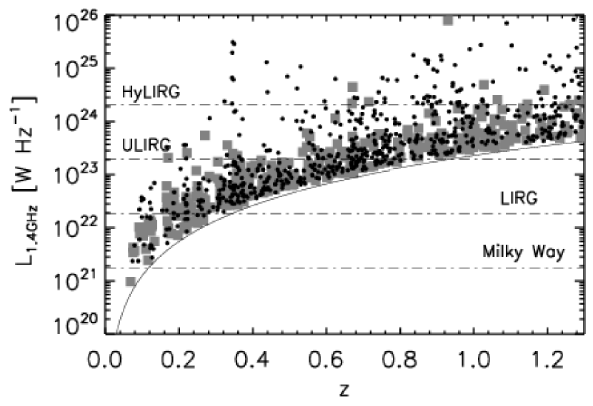
Figure 16.— 1.4 GHz luminosity as a function of redshift for the 340 selected star forming galaxies (grey squares) and 601 AGN (black dots). The horizontal (dot-dashed) lines correspond to 1.4 GHz luminosities typical for various classes of galaxies, obtained using the total IR – radio correlation (Bell, 2003). The solid curved line corresponds to the VLA-COSMOS $5\sigma$ limit of $\sim 50~{}\mathrm{\mu Jy}$. Note also that the VLA-COSMOS survey is sampling the entire LIRG and ULIRG populations out to redshifts of $\sim 0.4$ and $\sim 1$, respectively.

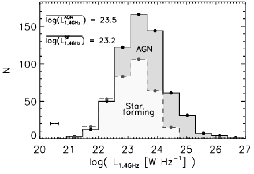
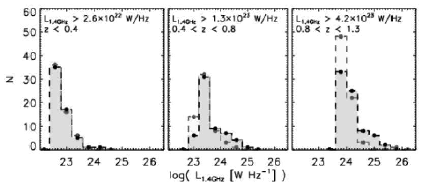
Figure 17.— Distribution of the logarithm of the 1.4 GHz luminosity for the selected star forming (light-grey shaded histograms) and AGN (dark-grey shaded histograms) galaxies for the entire flux limited sample (top panel), and for volume limited samples in 3 redshift ranges (bottom 3 panels). In the top panel the median $\log{\left(\mathrm{L}_{1.4\mathrm{GHz}}\right)}$ values for the full star forming and AGN samples, and the average error in $\log{\left(\mathrm{L}_{1.4\mathrm{GHz}}\right)}$ are indicated. The redshift and luminosity ranges of the volume limited samples are given in the bottom 3 panels.

Further, the luminosity distribution shown in Fig. 17 agrees well with local results, which have shown that $\mathrm{L}_{1.4\mathrm{GHz}}$ for star forming and (absorption and emission line) AGN shows overlapping distributions, and consequently no clear separation (e.g. Sadler et al. 1999; Jackson & Londish 2000; Chan et al. 2004). In the local universe Sadler et al. (1999) inferred a median $\mathrm{L}_{1.4\mathrm{GHz}}$ for SF and AGN galaxies to be $\sim 3\times 10^{22}$ W Hz^-1 and $\sim 3\times 10^{23}$ W Hz^-1, respectively. Hence, our median value for the luminosity of VLA-COSMOS AGN ($3.2\times 10^{23}$ W Hz^-1) out to $z=1.3$ matches the one inferred locally, however for SF galaxies ($1.6\times 10^{23}$ W Hz^-1) it is higher than that derived by Sadler et al. (1999). The latter is easily understood as the combined effect of the higher median redshift ($\sim 0.7$) of the galaxies in our flux limited sample (thus not probing low $\mathrm{L}_{1.4\mathrm{GHz}}$) and of the higher level of star formation activity, which is observed going from redshift 0 to 1 (Madau et al., 1996; Hopkins, 2004) also implying higher $\mathrm{L}_{1.4\mathrm{GHz}}$ (Condon, 1992; Bell, 2003).

We caution at this point that luminosity distributions of flux limited samples are strongly dependent on the detection limits, and their interpretation has to be approached carefully. For this reason, in Fig. 17 we also show the luminosity distributions for volume limited samples of our selected SF and AGN galaxies in three redshift ranges. On average AGN galaxies have higher 1.4 GHz luminosities than SF galaxies, reassuring the validity of our selection method. Note, however, that in the lowest redshift range the AGN and SF galaxy distributions are very similar. This is not surprising, but rather consistent with the observed luminosity range, that encompasses the region of indistinguishable space density of SF and AGN galaxies in the local universe (see local 1.4 GHz luminosity functions for SF and AGN galaxies; e.g. Best 2004).

7.2. The ’population mix’ in the VLA-COSMOS survey

In this Section we study the contribution of different sub-populations to the the total sub-mJy radio population. The key question we want to answer is: Is the sub-mJy population dominated by any particular sub-population, which may be the main cause for the observed flattening of the differential radio source counts below 1 mJy (for VLA-COSMOS source counts; see Bondi et al. 2007)?

7.2.1 Is the matched radio sample at sub-mJy levels dominated by star forming galaxies?

In order to obtain an insight into the ’population mix’ of the faint radio sources in the matched radio source sample, in Fig. 18 we show the distribution of the 1.4 GHz total flux density, $\mathrm{F_{tot}}$, for the SF and AGN galaxies in the matched radio sample out to $z=1.3$, as well as for the identified QSOs. Note, that the remaining $z>1.3$ galaxies in the matched radio sample are defined as high redshift (high-z) galaxies. The flux bins in Fig. 18 are 0.15 mJy wide. Such wide bins allow us to study the average behavior of the galaxies in the sub-mJy population with decreasing flux densities. Our main aim is to answer one of the more controversial questions in radio astronomy: Is the sub-mJy radio population dominated by star forming galaxies or any other distinct sub-population?

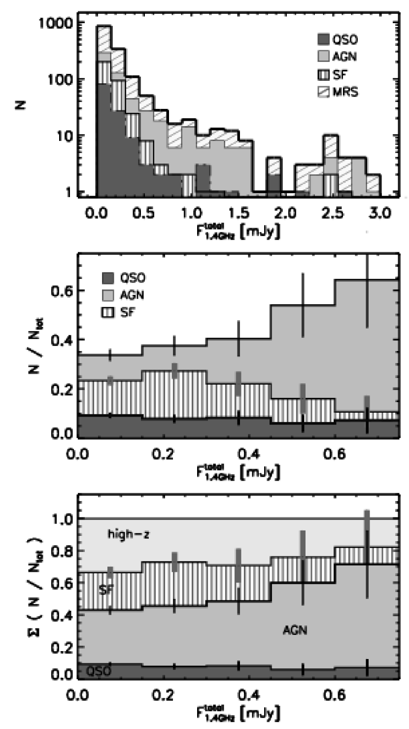
Figure 18.— Top: The distribution of the 1.4 GHz total flux for the star forming (vertically hatched histogram) and AGN galaxies (light-grey shaded histogram) in the matched radio sample out to $z=1.3$ (see also Fig. 17). Shown is also the distribution for the selected QSOs (dark-grey shaded histogram), for which good redshift information is not available at this point. ’MRS’ stands for the ’matched radio sample’. Middle: The relative contribution of SF, AGN galaxies out to $z=1.3$, and QSOs to the matched radio sample. Note that the missing fraction of sources consists of the high redshift (high-z) objects, which we define as galaxies in our matched radio sample with $z>1.3$. Bottom: The cumulative distribution of SF, AGN galaxies out to $z=1.3$, QSOs and high-z galaxies in the matched radio sample. The indicated error bars in the middle and bottom panels are derived from Poisson statistics. Note also the different flux scales in the top and the middle/bottom panels.

From the top panel in Fig. 18 it is obvious that at flux densities above $\sim 0.7$ mJy we are hampered by low number statistics (the total number of sources in each bin is below 20). Therefore, for the purpose of this paper we will focus only on sources with flux densities below $0.7$ mJy down to the VLA-COSMOS $5\sigma$ limit of $\sim 50~{}\mathrm{\mu}$Jy.

The middle panel in Fig. 18 shows the fractional distribution of the identified populations in the matched radio sample, with indicated Poisson errors. Our findings are as follows. QSOs contribute to the matched radio sample at a constant level of about $10\%$. AGN galaxies below $z=1.3$ show a decreasing trend with decreasing flux densities, with their contribution to the matched radio sample dropping from $\sim 60\%$ to less than $40\%$. The SF galaxies at $z\leq 1.3$ in the flux density range of $50~{}\mu$Jy to $0.7$ mJy contribute fairly constantly at the given flux densities, with an average contribution of about $20\%$. Note that the possible increment from $0.7$ mJy to $50~{}\mathrm{\mu}$Jy of only $\sim 10\%$ is not significant. In Sec. 4.2.2 we have inferred that the photometric errors in the synthesized $P1$ color introduce a positive bias of $\sim 5\%$ for SF galaxies. As this bin contains the lowest number of SF galaxies, it is the most affected by this bias. In Sec. 4.1.2, based on the local SDSS/NVSS sample of galaxies, we have shown that our rest-frame color based classification method selects $\sim 70\%$ of ’real’ SF galaxies, which make-up $\sim 85\%$ of the complete sample of SF galaxies, while the photometrically selected AGN sample is contaminated by SF galaxies at the $5\%$ level. Assuming that the percentages of completeness and contamination, derived from the analysis of the SDSS/NVSS sample of galaxies, can be safely applied also to our VLA-COSMOS sample, we can use them to correct the observed fractions. Even with the correction the fractional contribution of SF galaxies at $z<1.3$ in the matched radio population essentially stays the same, i.e. about $\sim 20\%$ at flux densities in the range from $50~{}\mathrm{\mu}$Jy to $0.7$ mJy. Contrary to previous studies (e.g. Seymour et al. 2004; Benn et al. 1993), our results show that SF galaxies at intermediate redshifts are not the dominant population at sub-mJy flux density levels. However, it may be possible that a significant number of SF galaxies at $z>1.3$ exists, which may contribute strongly to the sub-mJy population. We investigate this possibility in the bottom panel in Fig. 18 and in Fig. 19, and show below that this is not the case.

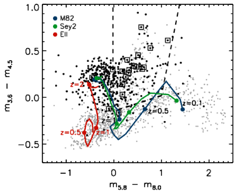
Figure 19.— MIR color – color digram (analogous to Fig. 10 , bottom panel) for the full matched radio sample. Gray dots represent sources classified using our classification method (i.e. SF and AGN galaxies out to $z=1.3$, and QSOs), while the black dots show the high-z sources (galaxies in the matched radio sample beyond $z=1.3$). Open black squares represent the high-z sources that have an XMM point source counterpart. The dashed lines are indicated to guide the eye, and correspond to the AGN type-1 selection region, proposed by Stern et al. (2005). The curved green, blue, and red lines correspond to the color-color tracks, obtained from SEDs of the starburst galaxy M 82, a composite of 28 Seyfert 2 galaxies, and a 13 Gyr old elliptical galaxy, respectively, in the redshift range from $0.1$ to $2.5$.

About $30\%$ of the matched radio sample consists of galaxies at redshifts beyond $z=1.3$ (high-z; see bottom panel in Fig. 18). The contribution of these galaxies marginally increases from 20% at 0.7 mJy to 35% at 50 $\mu$Jy. Although we were not able to apply our rest-frame color based classification method to these galaxies in order to classify them, we can nevertheless draw some conclusion about their nature by studying their multi-wavelength properties. Therefore, in Fig. 19 we plot the MIR diagnostic diagram, for the high-z galaxies and compare their properties to the classified sources in the matched radio sample. We overlay non-evolving color tracks for the typical starburst galaxy M82, an elliptical 13 Gyr old galaxy, and a Seyfert-2 type SED, obtained from a composite spectrum of 28 randomly chosen Seyfert galaxies (Polletta et al., 2006). As expected, the properties of high-z galaxies are consistent with properties of higher redshift ($z>1.5$) galaxies. However, the region they occupy in this MIR color-color diagram is occupied in a similar way by different sub-populations, such as star forming, Seyfert-type, and passively evolving galaxies, in the redshift range from about $1.5$ to $3$ (see color tracks in Fig. 19). Further, it is possible that a fraction of these sources are broad line AGN as they are located within the area outlined by dashed lines, which was proposed by Stern et al. (2005) for the selection of AGN Type-1 (see also Caputi et al. 2007). This is further strengthened by the 22 high-z sources which were also identified as X-ray point sources, and lie within the Type-1 AGN selection region. Further, given the high redshift of these sources, combined with the XMM detection limit, it is highly unlikely that any of these sources may be star forming (see e.g. Fig. 14 in Trump et al. 2007). This analysis alone already indicates that the matched radio sources beyond $z=1.3$ are most probably a mixture of different sub-populations.

The population mix in the high-z sample is further affirmed by the distribution of the high-z galaxies in the $BzK$ diagram (shown in Fig. 20), which is commonly utilized for the selection of $z>1.4$ galaxies, and separates well passively-evolving galaxies from those originally defined as ’star forming’ at $z>1.4$ (Daddi et al., 2004). Form Fig. 20 it becomes obvious that the BzK criterion does not select a pure ’star forming’ sample at $z>1.4$, as initially postulated, but a sample that is comprised of both SF galaxies and low-luminosity AGN. In addition, the X-ray detected high-z sources, which may be classified as AGN with high confidence as discussed above, also lie within this region. Therefore, the SED color tracks combined with the distribution of the high-z galaxies (black dots in Fig. 20), and the X-ray detected subsample suggest that our $z>1.3$ matched sources are a fair mixture of SF and AGN galaxies, yielding that the high-z galaxies continue to consist of different galaxy populations at higher redshifts.

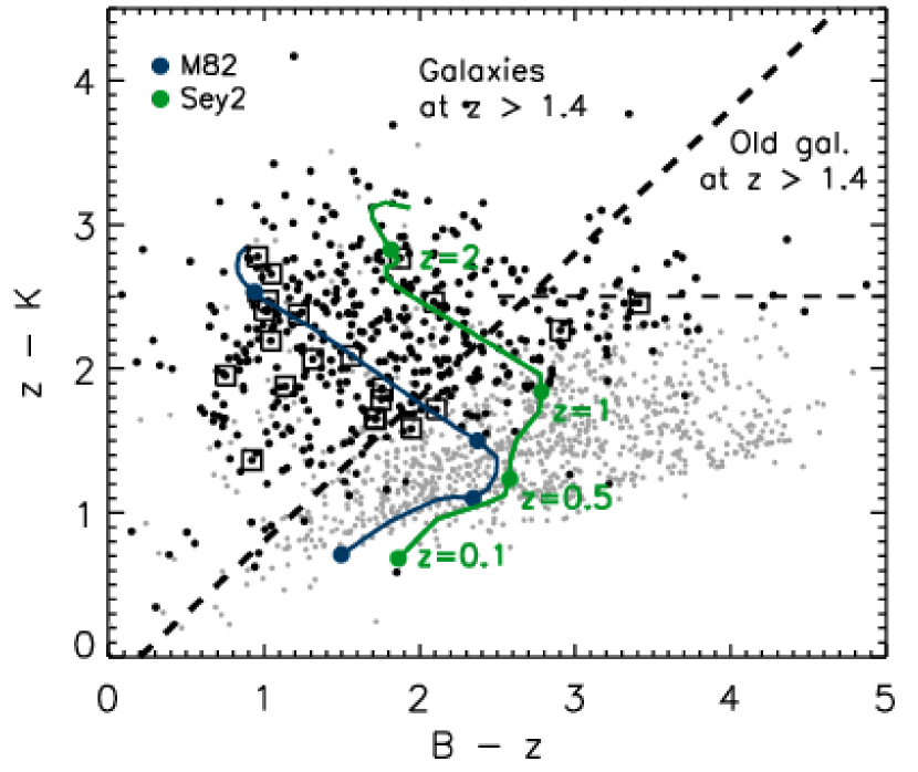
Figure 20.— $B-z$ vs. $z-K$ color-color diagram for the entire matched radio sample. The symbols are analogous to Fig. 19: Gray dots represent sources identified using our classification method (i.e. SF and AGN galaxies out to $z=1.3$, and QSOs), the black dots show the high-z sources, and open squares show XMM detected point sources in the high-z sample. The dashed lines separate regions of passively evolving (top right; outlined by the diagonal and horizontal dashed lines) and star-forming galaxies (left of the diagonal dashed line) at $z>1.4$, adopted from Daddi et al. (2004). The curved green and blue lines correspond to the color-color tracks, obtained from SEDs of the starburst galaxy M 82, and a Seyfert 2 composite, respectively, in the redshift range from $0.1$ to $2.5$. Note, that Seyfert type of galaxies at $z>1.4$ are also present in the region of ’star-forming galaxies’, as initially postulated by Daddi et al. (2004).

For reference, the $i$ band magnitude distribution for the identified sub-samples in the matched radio sample is shown in Fig. 21. Note that the high-z galaxies are the faintest optical sources, consistent with the expectations for high redshift sources drawn from a flux limited sample. However, we want to mention that even in the most extreme case that all of the high-z galaxies were star forming, still the fractional contribution of star forming galaxies to the matched radio source population would not dominate over the contribution of AGN and QSOs, but the two contributions would rather be comparable.

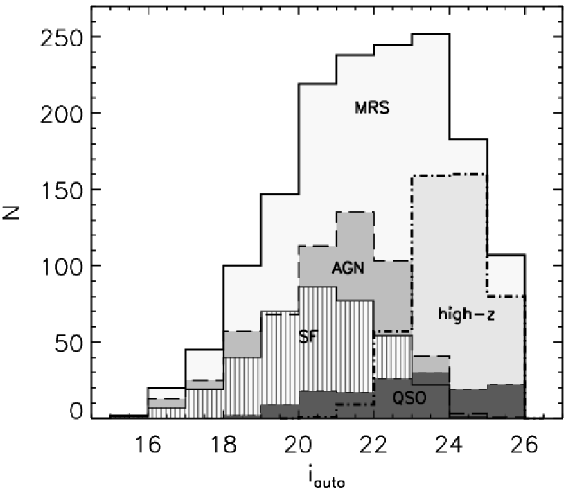
Figure 21.— Distribution of the $i$ band magnitude (Subaru where available, otherwise CFHT) for sources in the VLA-COSMOS matched radio sample (MRS). Also shown are the distributions for the identified sub-samples of sources: QSOs, star-forming (SF), AGN, and high-z galaxies

As shown in Fig. 20 it is likely that both classes of objects contribute similarly to the high-z galaxies, although their exact relative fractions cannot be determined from this analysis. However, if we assume that roughly $50\%$ of the high-z galaxies are SF galaxies, then the fraction of SF galaxies in the matched radio sample would increase to less than $40\%$. Therefore, we conclude that the population of star forming galaxies is not the dominant population at sub-mJy levels, at least in our sample of radio sources with optical counterparts out to $i=26$.

Our results are strikingly similar to the recent results by Padovani et al. (2007), who studied the sub-mJy radio source population in the Chandra Deep Field South down to a $5\sigma$ limit of $42~{}\mathrm{\mu}$Jy. They found that SF galaxies make up only about $20\%$ to $45\%$ (i.e. roughly 1/3) of the sub-mJy radio sources.

7.2.2 The contribution to the sub-mJy radio population from radio sources with no, or with flagged, optical counterparts

Most of the previous studies (as well as our study up to this point) of the faint radio population have relied on sub-samples of the observed radio sources, that have been identified with optical counterparts out to $i=26$, as representative of the entire sub-mJy radio population. For example, Benn et al. (1993) used a sample of only 87 out of 523 (i.e. less than $20\%$) 1.4 GHz radio sources above 0.1 mJy, for which they obtained optical spectroscopy ($B<22$), to conclude that above 1 mJy about $50\%$ of the galaxies were SF or Seyfert galaxies, while below 1 mJy the fraction increases to $\sim 90\%$. Further, Gruppioni et al. (1999) studied optical spectroscopic properties of 34 radio sources above $0.2$ mJy in the Marano Field down to $B=24$. This sample comprised $\sim 60\%$ of the entire sample of faint radio sources, and they concluded that the SF galaxies do not constitute the main galaxy population of their radio sources, and even at sub-mJy levels the majority of their radio sources were identified with early type galaxies, consistent with AGN. Gruppioni et al. attributed the difference in their results compared to the results from Benn et al. (1993) to the fainter optical magnitude limit reached for their radio sample. In this work we have an order of magnitude larger sample size (1558 sources with optical counterparts), and a significantly deeper optical limit ($i=26$) than previous studies. However, still our matched radio source sample consists of only $\sim 65\%$ of the VLA-COSMOS 1.4 GHz sources. Therefore, it is important to investigate the contribution of the remaining $\sim 35\%$ of the radio sources, with no identified or flagged optical counterparts, to the sub-mJy population. It may indeed be possible that a ’missing’ population of objects, that significantly contributes to the sub-mJy population, is ’hidden’ in this sample. We show below that this is not the case.

If the above hypothesis is true, then the properties (such as e.g. MIR colors) of these remaining objects are expected to be distinct from the properties of objects in the matched radio sample. In order to shed light on this, in Fig. 22 (top panel) we show the distribution of the total flux density for the 1558 sources in the matched radio sample, and for the remaining 830 sources that were a) not identified with optical counterparts with $i\leq 26$ or b) have optical counterparts with $i\leq 26$ but in photometrically masked-out region (see Sec. 3.1). The bottom panel shows the fractional contribution of these two samples compared to the entire VLA-COSMOS 1.4 GHz population. The fraction of matched radio sources is statistically consistent to be constant at $\sim 65\%$ at all faint flux density levels, although formally it decreased from $\sim 75\%$ at $\sim 0.7$ mJy to $\sim 60\%$ at the limit of the VLA-COSMOS survey. On the basis of these high percentages, it is unlikely that any further population, that is not present in our matched radio sample, could account for a significant fraction of the sub-mJy population.

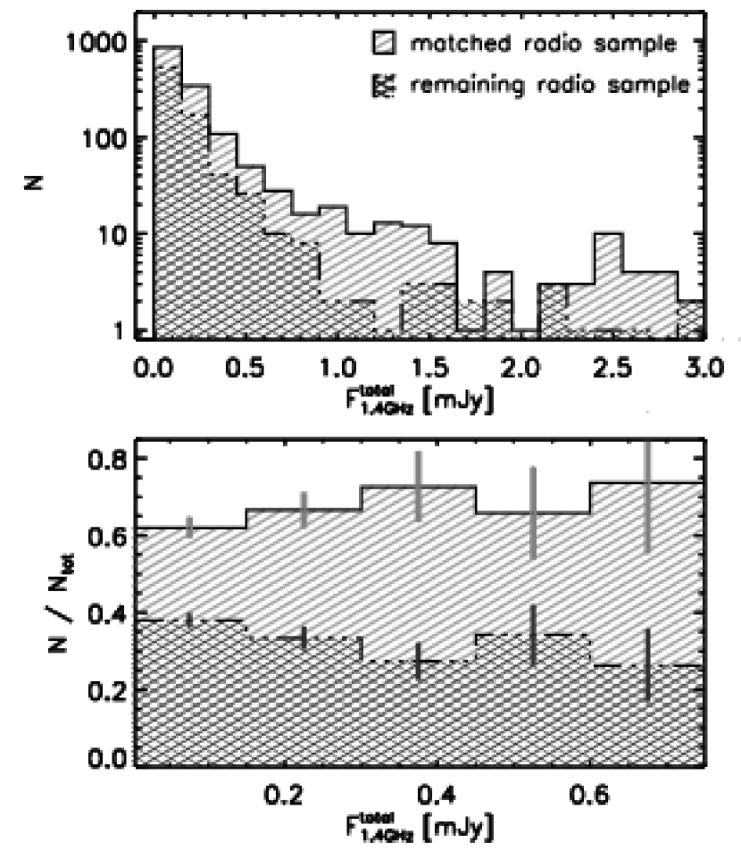
Figure 22.— Top: The distribution of the 1.4 GHz total flux for sources in the matched radio sample (single hatched histogram), and for other VLA-COSMOS sources that have either no identified, or a photometrically flagged, optical counterpart brighter than $i=26$ (cross-hatched histogram). Bottom: The fractional distribution of the two samples compared to the entire sample of 1.4 GHz radio sources. Indicated error bars are derived from Poisson statistics.

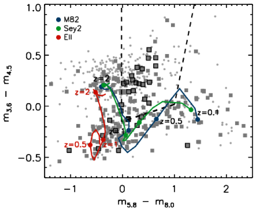
Figure 23.— Analogous to Fig. 19, but for $813$ VLA-COSMOS 1.4 GHz sources (grey dots) that have either no identified, or a photometrically flagged, optical counterpart brighter than $i=26$, but that have IRAC detections (i.e. $\sim 75\%$; see Sec. 3.4). Grey squares indicate the sources that have an optical counterpart with $i\leq 26$, but that is within a masked-out area. Black open squares represent the sources that have XMM point source detections. The clumping of objects in the upper left quadrant is consistent with both star forming, Seyfert and passive galaxies, in the redshift range from about $1.5$ to $3$, suggesting that over $\sim 60\%$ of the VLA-COSMOS ’remaining’ sources are high redshift galaxies or QSOs.

This is further strengthened by the distribution of the remaining sources in the MIR color-dolor diagram, shown in Fig. 23, which is consistent with the expected distribution for a mixed sample of star forming, AGN galaxies, and QSOs at all redshifts in the range from the local to the highest observable redshifts. An additional affirmation of the mix of population arises from the 31 sources that have been detected as X-ray point sources (see Fig. 23). It is worth noting however, that $\sim 60\%$ of these sources are consistent with higher redshift objects ($z\gtrsim 1.3$), while this is true only for $\sim 50\%$ of the galaxies in the matched radio sample (see Fig. 19). We therefore conclude that the radio sources without identified, or with flagged, optical counterparts brighter than $i=26$ are most likely comprised of a mixture of different source populations (SF, AGN, QSO), similar to, although on average at higher redshift then the radio sources in our matched radio sample. Further, the relatively small total percentage of these sources cannot significantly alter the results about the ’population mix’ in the 1.4 GHz VLA-COSMOS radio sample, inferred in the previous section.

7.3. Concluding remarks on the composition of the faint radio population

The faint – submillijansky – radio population comprises the radio population responsible for the upturn of the differential radio source counts below 1 mJy (see e.g. Bondi et al. 2007), and it has been the subject of many studies, and a matter of great debate in the past three decades (Condon, 1984; Windhorst et al., 1985; Gruppioni et al., 1999; Seymour et al., 2004; Simpson et al., 2006). This radio population has been interpreted as a ’new’ rising population of objects, that do not significantly contribute at higher radio flux density levels. However, results from studies that tried to reveal the exact composition of the sub-mJy population have been highly discrepant. It was suggested that the majority of this faint radio population consists of faint blue galaxies, and it was assumed that these galaxies are undergoing significant star formation (Windhorst et al., 1985). The spectroscopic study by Benn et al. (1993), although analyzing only less than $20\%$ of their radio sample, supported this result indicating that the fraction of SF and Seyfert galaxies rises from about $50\%$ to $90\%$ in the range from super- to sub-mJy flux densities. However, Gruppioni et al. (1999), who performed a deeper optical spectroscopic analysis of a larger fraction ($\sim 60\%$) of their radio sources, disagreed with this result identifying the majority of their sub-mJy radio sources with early type galaxies, in which the radio emission is produced by AGN. Recently, using a combination of optical and radio morphology as an identifier for AGN and SF galaxies on $\sim 90\%$ of their radio sources in the SSA13 field, Fomalont et al. (2006) suggested that less than $\sim 40\%$ of the radio sources below 1 mJy are AGN. On the other hand, Padovani et al. (2007) based their SF/AGN classification on a combination of optical morphologies, X-ray luminosities and radio–to–optical flux ratios of their radio sources in the CDFS (Chandra Deep Field South), and indicated that only about $20-40\%$ of the faint radio sources are made-up of star forming galaxies.

As already mentioned in the Sec. 1 there are two main reasons for such controversial results in the past literature: a) The identification fraction of radio sources with optical counterparts spans a wide range (20% to 90%) in samples from radio deep fields, and b) the methods for the separation of SF from AGN galaxies have been highly heterogeneous. Further, the first and second point seem to exclude each other. Namely, the most efficient separation methods (e.g. intermediate- to high- resolution optical spectroscopy) generally led to a small identification fraction, whereas large radio samples with high optical identification fractions usually lacked robust SF/AGN indicators. In this paper we have tried to make a strong conjunction of these two points. We introduced a new method to separate SF from AGN galaxies, which relies strongly on rest-frame color properties, and thus allowed us to perform a robust classification of $\sim 65\%$ ($=1558$) of the 1.4 GHz VLA-COSMOS radio sources down to $\sim 50~{}\mathrm{\mu Jy}$ with identified optical counterparts out to $i=26$ without the need for e.g. optical spectroscopy. Thus, we managed to reach both a high identification fraction and a robust source classification. However, in order to avoid any possible biases, we also utilized the full panchromatic COSMOS data set to put constraints on the properties of the remaining $\sim 35\%$ of the radio sources that were not identified with optical counterparts with $i\leq 26$, or that have optical counterparts with $i\leq 26$ but with uncertain photometry due to blending and saturation in the optical images. In short, we have obtained a complete view of the ’population mix’ of the sub-mJy radio sources, using to date the largest sample of 2388 faint ($5\sigma\approx 50~{}\mathrm{\mu}$Jy) radio sources at 1.4 GHz. Our combined methods allow us to reveal the true nature of the sub-mJy radio sources in the VLA-COSMOS survey on a sound statistical basis.

Jarvis & Rawlings (2004) first suggested that the observed flattening of the differential radio source counts below 1 mJy may be caused by ’radio-quiet’ AGN, i.e. radio-quiet QSOs and type-2 AGN (consistent with our ’AGN’ class), rather than star forming galaxies. Making use of the observed correlation between X-ray and radio luminosity and the empirically derived X-ray luminosity function, they computed the 1.4 GHz luminosity function for radio-quiet AGN out to high redshifts, and used it as the key ingredient to model the radio source counts at faint flux density levels (see Jarvis & Rawlings 2004 and references therein). However, they did not take into account SF galaxies as an important population to explain the shape of the counts. Such an interpretation managed to represent the differential radio source counts well down to $\sim 250~{}\mathrm{\mu Jy}$, but failed at fainter flux densities. Our results, derived in the previous sections, show that indeed star forming galaxies are not the dominant population at sub-mJy levels in the range of $50~{}\mathrm{\mu}$Jy to $0.7$ Jy, however they still contribute about $30\%$ to $40\%$ at these flux densities. Based on our large sample of 2388 VLA-COSMOS radio sources we find that our classified AGN, which comprise mostly of low-luminosity and type-2 AGN, make up $50-60\%$ of the faint radio population with a decreasing trend towards fainter flux densities, while the identified QSOs, which are mostly type-1 AGN, form a minor contribution of $\sim 10\%$ of the sub-mJy radio population in the range of $50~{}\mathrm{\mu}$Jy to $0.7$ Jy. Thus, our observational results show that the ’population mix’ in the faint radio population contains a fair contribution of both SF galaxies and (low-luminosity and obscured) AGN, at least down to $50~{}\mathrm{\mu}$Jy. Thus, separate luminosity functions for both populations have to be taken into account in order to fully explain the flattening of the radio source counts below 1 mJy. The 1.4 GHz luminosity function for star forming and AGN galaxies at intermediate redshift, as well as the modeling of the 1.4 GHz radio source counts using these new observational constrains and further analyzes of the ’population mix’ in the VLA-COSMOS survey, is going to be fully addressed and presented in a number of up-coming publications (Smolčić et al., 2007; Ciliegi et al., 2007b; Paglione et al., 2007).

8. Summary

Our newly developed rest-frame color based classification method, in conjunction with the VLA-COSMOS 1.4 GHz observations, enabled us to make, for the first time, a thorough distinction between sources where the 1.4 GHz radio emission is predominantly driven by star formation processes from those where it is driven by SMBH processes, regardless of the luminosity of the latter, and apply it to currently the largest sample of 1558 1.4 GHz sources, with optical counterparts brighter than $i_{\mathrm{AB}}\leq 26$, and complete down to $\sim 50~{}\mathrm{\mu Jy}$.

We have explored to full detail the composition of the sub-mJy radio population making use of the entire sample of 2388 VLA-COSMOS radio sources detected above $5\sigma~{}(\approx 50\mathrm{\mu Jy})$, in conjunction with the panchromatic (X-ray to radio) COSMOS data set. We find that SF galaxies are not the dominant population at submillijansky flux density levels, as believed previously, but that they rather make up an approximately constant fraction of $30-40\%$ in the flux density range of $\sim 50~{}\mathrm{\mu}$Jy to $0.7$ mJy. The radio population at these flux densities is a mixture of roughly $30-40\%$ of SF and $50-60\%$ of AGN galaxies, with a minor contribution ($\sim 10\%$) of QSOs.

Table 1 Multi-wavelength cross-correlation of VLA-COSMOS 1.4 GHz radio sources

	total	$z_{\mathrm{spec}}$	IRAC	MIPS	XMM
total radio sample	2388	520	2058	1117	210
matched radio sample	1558	447	1448	799	179
stars	2	0	2	2	0
QSOs	139	31	122	78	43
SF galaxies	340	150	322	280	16
AGN galaxies	601	262	579	267	98
high-z galaxies	476	4	423	172	22
remaining radio sample	830	73	610	318	31

Appendix A The rest-frame colors $P1$ and $P2$

The rest-frame colors $P1$ and $P2$ are a a linear superposition of colors in the wavelength range of 3500 – 5800 Å, obtained using the modified Strömgren photometric system (Odell et al., 2002; Smolčić et al., 2006, the filter response curves are available at http://www.mpia-hd.mpg.de/COSMOS). $P1$, $P2$ are principal component axes optimally characterizing the galaxy locus in 2D color-color space. $P1$ measures the position along the galaxy locus, and $P2$ the position perpendicular to it (see Fig. 4 in Smolčić et al. 2006). As the galaxy locus is slightly curved, the functional form of the rest-frame colors is given separately for the blue and red ends, with a boundary at $vz-yz=0.646$. Hence, for galaxies with $vz-yz\leq 0.646$ ($P1$,$P2$) are given as:

$$P1=\phantom{X}0.911\,(c_{1}-0.646)+0.412\,(c_{2}-0.261)$$ (A1)

$$P2=-0.412\,(c_{1}-0.646)+0.911\,(c_{2}-0.261),$$ (A2)

and for galaxies with $vz-yz>0.646$ as:

$$P1=\phantom{X}0.952\,(c_{1}-0.646)+0.307\,(c_{2}-0.261)$$ (A3)

$$P2=-0.307\,(c_{1}-0.646)+0.952\,(c_{2}-0.261),$$ (A4)

where $c_{1}=vz-yz$ and $c_{2}=bz-yz$.

Appendix B Derivation of completeness and contamination of the photometrically selected samples of star forming galaxies and AGN

B.1. SDSS/NVSS galaxy sample

Given both the available spectroscopy and photometry of the local galaxy sample (SDSS/NVSS) we can easily access the completeness and contamination of the photometrically selected samples of SF and AGN galaxies as follows. In Fig. 24 we show the differential and cumulative distributions of $P1$ for the SDSS/NVSS star forming, composite and AGN galaxies. Here the classification is based on the BPT diagram for the galaxies with emission lines in their spectra, while all galaxies without emission lines are included in the AGN class. These ’absorption line AGN’ constitute the major fraction of all the AGN ($\sim 80\%$) in the sample. The top panel shows the $P1$ histograms for these three types of objects, normalized by the total number of objects. In the middle panels in Fig. 24 we show the fractions for the SF, AGN and composite galaxies for the selection of SF (left panel) and AGN (right panel) galaxies. The fractions were computed in such a way that for each $P1$ value ($P1_{i}$) the distributions were normalized to the total number of galaxies in the sample with $P1\leq P1_{i}$ (for SF galaxies; left panel), or $P1>P1_{i}$ (for AGN galaxies; right panel). In this way, we obtain the fraction of SF, AGN and composite galaxies within the full sample that was selected only by applying a $P1$ color-cut. Further, in the bottom panels in Fig. 24 we show the cumulative distributions of the SF (left panel) and AGN (right panel) galaxies, scaled to the total number of SF and AGN galaxies, respectively, thus showing their completeness as a function of $P1$. Selecting galaxies with $P1$$\leq$$0.15$, and defining them as the ’photometrically selected sample of star forming galaxies’, leads to a sample that contains $\sim 20\%$ AGN, $\sim 10\%$ composite objects, and $\sim 70\%$ ’real’ (i.e. spectroscopically identified) SF galaxies (see middle left panel in Fig. 24). The latter make-up $\sim 85\%$ of all ’real’ SF galaxies (see bottom left panel in Fig. 24). On the other hand, using the color cut to generate the ’photometrically selected AGN galaxy sample’ ($P1$$>$$0.15$) leads to a sample that contains $\sim 5\%$ SF galaxies, $\sim 15\%$ composite objects, and $\sim 80\%$ ’real’ AGN galaxies (see middle right panel in Fig. 24), where the latter make-up $\sim 90\%$ of all ’real’ AGN galaxies (see bottom right panel in Fig. 24).

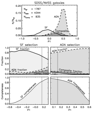
Figure 24.— Differential and cumulative distributions of the rest-frame color $P1$ for $\sim 7,000$ SDSS galaxies, in the redshift range of $0.01$ to $0.3$, drawn from the DR1 “main” spectroscopic sample, that have 1.4 GHz NVSS detections. The galaxies were spectroscopically classified as star forming (SF; thick line), AGN (dashed line) or composite (dot-dashed line; see text for details). The top panel shows the $P1$ histograms for these three types of objects. The middle left panel shows the fraction of these three types of galaxies as a function of $P1$. These distributions are normalized in such a way that for each $P1$ value the fraction of the three types of galaxies within the total selected sample can be read off. The bottom left panel shows the cumulative distribution of $P1$ for SF galaxies, thus showing to which completeness the ’real’ (i.e. spectroscopically classified) SF galaxies are selected for any given $P1$ color-cut. The bottom and middle right panels are analogous to the bottom and middle left panels, but for AGN galaxies. Note also that the cumulative distributions for AGN were computed as a function of decreasing $P1$. The vertical (thin solid) lines in the middle and bottom panels designate the value of $P1$, chosen to separate SF galaxies from AGN.

B.2. SDSS/NVSS/IRAS galaxy sample

The BPT diagram for $\sim 830$ SDSS/NVSS/IRAS emission line galaxies is shown in Fig. 25, color-coded using the ($P1$,$P2$) plane. A strong correlation between $P1$ and $\log{\left(\mathrm{[NII\,\,6584]/H\alpha}\right)}$, very similar to the correlation observed for the full sample, is discernible.

The differential distribution of $P1$ for the complete sample of 875 SDSS/NVSS/IRAS galaxies is shown in the top panel of Fig. 24. The galaxies were spectroscopically separated into AGN, star-forming and composite galaxies (as described in Sec. 4.1.1). In the middle panel we show the corresponding fraction (analogous to the middle left panel in Fig. 24). Using a rest-frame $P1$ color cut-off of $0.15$ the selected sample of star forming galaxies, detected in the IR regime, contains $\sim 70\%$ ’real’ (i.e. spectroscopically identified) SF galaxies (that make up $\sim 85\%$ of all ’real’ SF galaxies; see bottom panel), $10\%$ AGN, and $20\%$ composite objects. This is fairly consistent with the properties of the entire SDSS/NVSS sample.

In order to assess the fraction of dusty starburst galaxies that we omit using the rest-frame color selection, in the bottom panel of Fig. 26 we show the cumulative distributions of the spectroscopically identified star forming galaxies as a function of $P1$ for i) all star forming galaxies, ii) luminous IR galaxies (LIRGs; $\mathrm{L_{IR}}=10^{11-12}$ $\mathrm{L}_{\odot}$) and iii) ultra-luminous IR galaxies (ULIRGs, $\mathrm{L_{IR}}>10^{12}$ $\mathrm{L}_{\odot}$). [The total IR luminosities were computed following Sanders & Mirabel (1996).] A $P1$ cut of $0.15$ misses only $\sim 10\%$ and $\sim 5\%$ of luminous and ultra-luminous starburst galaxies, respectively.

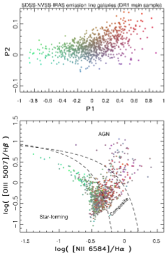
Figure 25.— Analogous to Fig. 4 but for $\sim 830$ SDSS/NVSS/IRAS emission line galaxies.

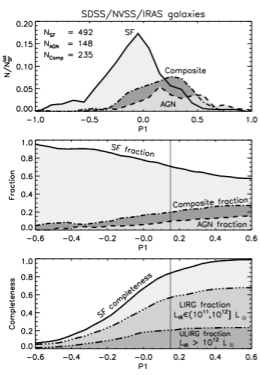
Figure 26.— Differential and cumulative distributions of the rest-frame color $P1$ for $875$ SDSS galaxies from the DR1 “main” spectroscopic sample, that have NVSS and IRAS detections. The galaxies were spectroscopically classified as star forming (SF; thick line), AGN (dashed line) or composite (dot-dashed line; see text for details), and their $P1$ histograms are shown in the top panel. The middle panel shows the fraction of $P1$ for SF, AGN and composite galaxies, analogous to the middle left panel in Fig. 24. The vertical thin solid line shows the chosen $P1$ color cut-off. The bottom panel shows the cumulative distribution of $P1$, normalized to SF galaxy counts (thick line). Also shown are the $P1$ distributions of SF galaxies with IR luminosities greater than  $10^{11}$ $\mathrm{L}_{\odot}$ and $10^{12}$ $\mathrm{L}_{\odot}$  consistent with LIRGs and ULIRGs, respectively. Note that our rest-frame color based classification method is not strongly biased against dusty starburst galaxies.

References

- Abazajian et al. (2003) Abazajian, K., et al. 2003, AJ, 126, 2081
- Abazajian et al. (2004) Abazajian, K., et al. 2004, AJ, 128, 502
- Abazajian et al. (2005) Abazajian, K., et al. 2005, AJ, 129, 1755
- Adelman-McCarthy et al. (2006) Adelman-McCarthy, J. K., et al. 2006, ApJS, 162, 38
- Alexander et al. (2001) Alexander, D. M., Brandt, W. N., Hornschemeier, A. E., Garmire, G. P., Schneider, D. P., Bauer, F. E., & Griffiths, R. E. 2001, AJ, 122, 2156
- Appleton et al. (2004) Appleton, P. N., et al. 2004, ApJS, 154, 147
- Arnouts et al. (2002) Arnouts, S., et al. 2002, MNRAS, 329, 355
- Baldwin, Phillips & Terlevich (1981) Baldwin, J. A., Phillips, M. M., & Terlevich, R. 1981, PASP, 93, 5
- Beichman et al. (1981) Beichman et al. 1985, IRAS Catalogs and Atlases, US GPO, Washington DC
- Becker et al. (1995) Becker, R. H., White, R. L., & Helfand, D. J. 1995, ApJ, 450, 559
- Beichman et al. (1985) Beichman, C. A., Neugebauer, G., Habing, H. J., Clegg, P. E. & Chester, T. J., 1985, IRAS Catalogs and Atlases (US GPO, Washington, DC
- Bell (2003) Bell, E. F. 2003, ApJ, 586, 794
- Benn et al. (1993) Benn, C. R., Rowan-Robinson, M., McMahon, R. G., Broadhurst, T. J., & Lawrence, A. 1993, MNRAS, 263, 98
- Benz & Guedel (1994) Benz, A. O., & Guedel, M. 1994, A&A, 285, 621
- Berger (2006) Berger, E. 2006, ApJ, 648, 629
- Best (2004) Best, P. N. 2004, MNRAS, 351, 70
- Best et al. (2005a) Best, P. N., Kauffmann, G., Heckman, T. M., & Ivezić, Ž. 2005, MNRAS, 362, 9
- Brinchmann et al. (2004) Brinchmann, J., Charlot, S., White, S. D. M., Tremonti, C., Kauffmann, G., Heckman, T., & Brinkmann, J. 2004, MNRAS, 351, 1151
- Brusa et al. (2007a) Brusa, M., et al. 2007, ApJS, 172, 353
- Brusa et al. (2007b) Brusa, M., et. al. 2007, in prep
- Bruzual & Charlot (2003) Bruzual, G., & Charlot, S. 2003, MNRAS, 344, 1000
- Bondi et al. (2007) Bondi, M., et. al. 2007, in prep
- Capak et al. (2007) Capak, P., et. al. 2007, ApJS, COSMOS special issue, in press
- Capak et al. (2007b) Capak, P., et. al., in prep
- Cappelluti et al. (2007) Cappelluti, N., et al. 2007, ArXiv Astrophysics e-prints, arXiv:astro-ph/0701196
- Caputi et al. (2007) Caputi, K. I., et al. 2007, ApJ, 660, 97
- Chan et al. (2004) Chan, B. H. P., Cram, L. E., Sadler, E. M., Killeen, N. E. B., Jackson, C. A., Mobasher, B., & Ekers, R. D. 2004, MNRAS, 352, 1245
- Ciliegi et al. (2007a) Ciliegi, P., et. al. 2007, in prep
- Ciliegi et al. (2007b) Ciliegi, P., et. al. 2007, in prep
- Clewley & Jarvis (2004) Clewley, L., & Jarvis, M. J. 2004, MNRAS, 352, 909
- Colless et al. (2001) Colless, M., et al. 2001, MNRAS, 328, 1039
- Condon (1984) Condon, J. J. 1984, ApJ, 287, 461
- Condon (1992) Condon, J. J. 1992, ARA&A, 30, 575
- Condon et al. (1998) Condon, J.J., Cotton, W.D., Greisen, E.W., Yin, Q.F., Perley, R.A., Taylor, G.B., Broderick, J.J., 1998, AJ, 115, 1693
- Daddi et al. (2004) Daddi, E., Cimatti, A., Renzini, A., Fontana, A., Mignoli, M., Pozzetti, L., Tozzi, P., & Zamorani, G. 2004, ApJ, 617, 746
- Dunlop & Peacock (1990) Dunlop, J. S., & Peacock, J. A. 1990, MNRAS, 247, 19
- Fanaroff & Riley (1974) Fanaroff, B. L., & Riley, J. M. 1974, MNRAS, 167, 31P
- Finoguenov et al. (2007) Finoguenov, A., et al. 2007, ApJS, 172, 182
- Fioc & Rocca-Volmerange (1997) Fioc, M., & Rocca-Volmerange, B. 1997, A&A, 326, 950
- Fomalont et al. (2006) Fomalont, E. B., Kellermann, K. I., Cowie, L. L., Capak, P., Barger, A. J., Partridge, R. B., Windhorst, R. A., & Richards, E. A. 2006, ApJS, 167, 103
- Franzetti (2005) Franzetti P., 2005, PhD thesis, Universita’ di Milano-Bicocca, Milano
- Gruppioni et al. (1999) Gruppioni, C., Mignoli, M., & Zamorani, G. 1999, MNRAS, 304, 199
- Guedel & Benz (1993) Guedel, M., & Benz, A. O. 1993, ApJ, 405, L63
- Güdel (2002) Güdel, M. 2002, ARA&A, 40, 217
- Guzzo et al. (2007) Guzzo, L., et al. 2007, ApJS, 172, 254
- Haarsma et al. (2000) Haarsma, D. B., Partridge, R. B., Windhorst, R. A., & Richards, E. A. 2000, ApJ, 544, 641
- Hasinger et al. (2007) Hasinger, M., et. al. 2007, ApJS, COSMOS special issue, in press
- Hauschildt et al. (1997) Hauschildt, P. H., Baron, E., & Allard, F. 1997, ApJ, 483, 390
- Hopkins et al. (2003) Hopkins, A. M., et al. 2003, ApJ, 599, 971
- Hopkins (2004) Hopkins, A. M. 2004, ApJ, 615, 209
- Ilbert et al. (2006) Ilbert, O., et al. 2006, A&A, 457, 841
- Ilbert et al. (2007) Ilbert, O., et al., in prep
- Impey et al. (2007) Impey, C. D., et al. 2007, IAU Symposium, 238, 287
- Ivezić et al. (2002) Ivezić, Ž., et al. 2002, AJ, 124, 2364
- Ivison et al. (2007) Ivison, R. J., et al. 2007, ApJ, 660, L77
- Jackson & Londish (2000) Jackson, C. A., & Londish, D. M. 2000, Publications of the Astronomical Society of Australia, 17, 234
- Jarvis & Rawlings (2004) Jarvis, M. J., & Rawlings, S. 2004, New Astronomy Review, 48, 1173
- Kauffmann et al. (2003) Kauffmann, G., et al. 2003, MNRAS, 346, 1055
- Kewley et al. (2001) Kewley, L. J., Dopita, M. A., Sutherland, R. S., Heisler, C. A., & Trevena, J. 2001, ApJ, 556, 121
- Koekemoer et al. (2007) Koekemoer, E., et. al. 2007, ApJS, COSMOS special issue, in press
- Kong et al. (2004) Kong, X., Charlot, S., Brinchmann, J., & Fall, S. M. 2004, MNRAS, 349, 769
- Lacy et al. (2004) Lacy, M., et al. 2004, ApJS, 154, 166
- Leauthaud et al. (2007) Leauthaud, A., et. al. 2007, ApJS, COSMOS special issue, in press
- Le Floc’h et al. (2005) Le Floc’h, E., et al. 2005, ApJ, 632, 169
- Lilly et al. (2007) Lilly, E., et. al. 2007, ApJS, COSMOS special issue, in press
- Madau et al. (1996) Madau, P., Ferguson, H. C., Dickinson, M. E., Giavalisco, M., Steidel, C. C., & Fruchter, A. 1996, MNRAS, 283, 1388
- Maccacaro et al. (1988) Maccacaro, T., Gioia, I. M., Wolter, A., Zamorani, G., & Stocke, J. T. 1988, ApJ, 326, 680
- Cappelluti et al. (2007) Cappelluti, E., et. al. 2007, ApJS, COSMOS special issue, in press
- Odell et al. (2002) Odell, A. P., Schombert, J., & Rakos, K. 2002, AJ, 124, 3061
- Obrić et al. (2006) Obrić, M., et al. 2006, MNRAS, 370, 1677
- Padovani et al. (2007) Padovani, P., Mainieri, V., Tozzi, P., Kellermann, K. I., Fomalont, E. B., Miller, N., Rosati, P., & Shaver, P. 2007, ArXiv Astrophysics e-prints, arXiv:astro-ph/0701493
- Paglione et al. (2007) Paglione et al., in prep
- Peterson (1997) Peterson, B. M. 1997, An introduction to active galactic nuclei, Publisher: Cambridge, New York Cambridge University Press, 1997 Physical description xvi, 238 p. ISBN 0521473489,
- Polletta et al. (2006) Polletta, M. d. C., et al. 2006, ApJ, 642, 673
- Prescott et al. (2006) Prescott, M. K. M., Impey, C. D., Cool, R. J., & Scoville, N. Z. 2006, ApJ, 644, 100
- Salpeter (1955) Salpeter, E. E. 1955, ApJ, 121, 161
- Richards et al. (2002) Richards, G. T., et al. 2002, AJ, 123, 2945
- Rola, Terlevich & Terlevich (1997) Rola, C. S., Terlevich, E., & Terlevich, R. J. 1997, MNRAS, 289, 419
- Sadler et al. (1999) Sadler, E. M., McIntyre, V. J., Jackson, C. A., & Cannon, R. D. 1999, Publications of the Astronomical Society of Australia, 16, 247
- Salim et al. (2007) Salim et al. 2007, submitted to ApJS
- Salvato et al. (2007) Salvato, M. et al., in prep
- Sanders & Mirabel (1996) Sanders, D. B., & Mirabel, I. F. 1996, ARA&A, 34, 749
- Sanders et al. (2007) Sanders, E., et. al. 2007, ApJS, COSMOS special issue, in press
- Schiminovich et al. (2007) Schiminovich et al., in prep
- Seymour et al. (2004) Seymour, N., McHardy, I. M., & Gunn, K. F. 2004, MNRAS, 352, 131
- Schinnerer et al. (2007) Schinnerer, E., et. al. 2007, ApJS, COSMOS special issue, in press
- Schneider et al. (2005) Schneider, D. P., et al. 2005, AJ, 130, 367
- Scoville et al. (2007a) Scoville, E., et. al. 2007, ApJS, COSMOS special issue, in press
- Scoville et al. (2007b) Scoville, N., et al. 2007, ApJS, 172, 150
- Silva et al. (1998) Silva, L., Granato, G. L., Bressan, A., & Danese, L. 1998, ApJ, 509, 103
- Simpson et al. (2006) Simpson, C., et al. 2006, MNRAS, 372, 741
- Smolčić et al. (2004) Smolčić, V., et al. 2004, ApJ, 615, L141
- Smolčić et al. (2006) Smolčić, V., et al. 2006, MNRAS, 371, 121
- Smolčić et al. (2007) Smolčić, V., et al. 2007, in prep
- Smolčić et al. (2007b) Smolčić, V., et al. 2007, ApJS, 172, 295
- Stern et al. (2005) Stern, D., et al. 2005, ApJ, 631, 163
- Stoughton et al. (2002) Stoughton, C., et al. 2002, AJ, 123, 485
- Strateva et al. (2001) Strateva, I., et al. 2001, AJ, 122, 1861
- Strauss et al. (2002) Strauss, M. A., et al. 2002, AJ, 124, 1810
- Szkody et al. (2002) Szkody, P., et al. 2002, AJ, 123, 430
- Szkody et al. (2003) Szkody, P., et al. 2003, AJ, 126, 1499
- Szkody et al. (2004) Szkody, P., et al. 2004, AJ, 128, 2443
- Taniguchi et al. (2007a) Taniguchi, Y., et al. 2007, ApJS, 172, 9
- Taniguchi et al. (2007b) Taniguchi, L., et al. 2007, in prep
- Tasca et al. (2007) Tasca, L., et al. 2006, MNRAS, 371, 121
- Tran et al. (2001) Tran, Q. D., et al. 2001, ApJ, 552, 527
- Tremonti et al. (2004) Tremonti, C. A., et al. 2004, ApJ, 613, 898
- Trump et al. (2007) Trump, J. R., et al. 2007, ApJS, 172, 383
- Veilleux & Osterbrock (1987) Veilleux, S., & Osterbrock, D. E. 1987, ApJS, 63, 295
- Veilleux et al. (1999) Veilleux, S., Sanders, D. B., & Kim, D.-C. 1999, ApJ, 522, 139
- Willott et al. (2002) Willott, C. J., Rawlings, S., Blundell, K. M., Lacy, M., Hill, G. J., & Scott, S. E. 2002, MNRAS, 335, 1120
- Windhorst et al. (1985) Windhorst, R. A., Miley, G. K., Owen, F. N., Kron, R. G., & Koo, D. C. 1985, ApJ, 289, 494
- Zamojski et al. (2007) Zamojski, E., et. al. 2007, ApJS, COSMOS special issue, in press
- York et al. (2000) York, D. G., et al. 2000, AJ, 120, 1579
- Yun & Carilli (2002) Yun, M. S., & Carilli, C. L. 2002, ApJ, 568, 88