Numerical approximations to extremal metrics on toric surfaces
1 Introduction
This is a report on numerical work on extremal Kahler metrics on toric surfaces, using the ideas developed in [3]111Although the simpler results described here were obtained by the second author in 2004, before those of [3].. These are special Riemannian metrics on manifolds of real, or complex dimensions. They can be regarded as solutions of a fourth order partial differential equation for a convex function on a polygon. We refer to the preceding article [4] for further background. Motivation for this kind of work can be found in at least three different sources:
-
•
Great effort is expended on the proof of abstract existence theorems for such metrics. Only very rarely does one expect to find explicit formulae for the solutions. It is interesting to explore the geometry of the solutions using numerical methods.
-
•
It is conceivable that specific numerical results of this general nature could be relevant to physics [7].
-
•
The numerical work illuminates the analytical techniques and difficulties involved in the abstract existence theory. This is true both of the approximate numerical solutions and of the approximation scheme itself, which is founded on a link between algebraic geometry and asymptotic analysis.
The results described here are obtained using a computer programme which can be applied in principle to any polygon and in practice works effectively for a reasonable range of cases. We focus on four such cases: particular -sided polygons with , which correspond to complex surfaces constructed by “blowing up” the projective plane times. The status of the rigorous existence theory is different in the four cases:
-
•
For the hexagon, the metric we seek is a Kahler-Einstein metric whose existence was proved by Tian, Yau and Siu in the 1980’s. Using a rather different approach, Doran et al [6] also recently found numerical approximations to this metric.
-
•
For the pentagon the metric we seek was proved to exist very recently by Chen, LeBrun and Weber [1]
-
•
For the octagon, the metric we seek has constant scalar curvature and the abstract existence follows from recent work of the second author.
-
•
For the heptagon, the metric we seek is extremal but not constant scalar curvature, and as far as we know is not at present covered by any general existence theorem.
But we emphasise that these cases are just a small sample of the ones that can be treated successfully, and there are many other cases of the fourth kind, where the numerical results outrun, at present, the abstract existence theory.
In each of these four cases we give a selection of geometrical results: again these form a small sample of what one can do. The pentagon is particularly interesting because, as Chen, Le Brun and Weber showed, it yields a new (conformally-Kahler) solution to the Riemannian Einstein equations. (More precisely, the extremal metric we approximate is very close to another extremal metric which is conformal to an Einstein metric.) We verify this numerically. from which one could go on to obtain information about the Einstein metric.
In the final section, we make some comments about ways in which these techniques might be taken further in the future.
We are grateful to Julien Keller for many discussions about this work, and much crucial technical assistance. In particular, the C++ version of the programme to find geodesics was written by Keller.
2 The set-up
2.1 Algebraic metrics
Our starting point is an integral Delzant polygon , contained in the square of side length . So for example, this is a picture of our hexagon, with .
When we write, for example, “the hexagon with ”, we mean the same figure scaled up by a factor of . So, for the hexagon, we can take to be any even number (because we need to work with polygons having integral vertices). This use of language differs slightly from that in [4], but we hope the meaning will be clear. We also indicate in the diagram the self-intersection numbers of the -spheres in the manifold corresponding to the edges; in this case all .
Next we consider a collection of positive numbers indexed by the lattice points in the closed polygon . Then we define a “Kahler potential”
This a convex function (of a variable ) whose derivative maps onto the polygon . The Kahler potential defines an “algebraic metric” on the toric surface corresponding to . The Legendre transform of is a convex function on . The scalar curvature is given by the expression . If were to satisfy the partial differential equation
| (1) |
for an affine linear function , then our metric would be extremal. This occurs in two very special cases:
-
•
If is the rectangle, with origin as one vertex, then we can take the product of binomial coefficients
for integers .
-
•
If is the triangle with vertices we can take the multinomial co-efficents
The metrics we describe are, respectively, the product of round metrics on and the Fubini-Study metric on . These are extremal metrics but of course we have not really gained anything new. In general, we cannot hope to find an extremal metric exactly, in this way, but we can hope to find good approximations, and we can hope that the approximations improve when we increase . For example, this is a collection of co-efficients which give a good approximation to the extremal metric in the case of the hexagon, for :
In this case there is a symmetry under a dihedral group of order 12, so we can reduce to only 6 independent coefficients. For clarity we have just written these to a few significant figures. When is larger the data is best kept confined to a computer file, and we will just record the maximum and minimum of the . It may be helpful to recall here from [5] that the numbers can be thought of, roughly, as a “discrete approximation” to the symplectic potential . Saying much the same thing in a different way, if we view as a function on depending on parameters , then at a given point the value of is strongly influenced by the for close to , but only little by those for far away . These somewhat vague statements become more precisely true when the parameter is large.
If is any affine-linear function then changing the coefficients to does not change the metric described by the data. We can normalise the to take account of this, as follows. Let be the centre of mass of the polygon. We arrange that
| (2) |
2.2 Decomposition of the curvature tensor
Here we want to extend slightly the discussion of the curvature tensor of a toric manifold in [4], for the two-dimensional case.
We begin in a more general setting and consider a complex Kahler surface with an anti-holomorphic isometric involution fixing a submanifold of two real dimensions. Thus is a “real form” of . We want to understand the curvature tensor of at a point of . We have where is the normal bundle. Fix an orientation of , at least locally. This determines an orientation of the normal bundle so, using the metric, we can define complex structures on each of and , making them complex line bundles. With suitable choice of signs the resulting complex structure on induces the opposite orientation on from that of the Kahler structure. Thus we have a unit anti-self-dual -form at and we can write
say, where is a two-dimensional oriented real vector space. Thinking of as the complexification of we see that there is a natural map from the trace-free symmetric -tensors to the trace-free Hermitian forms on at . In a standard basis this is just the obvious map which takes a symmetric real matrix to a Hermitian matrix. It is easy to check that the image of this is , so we can identify with .
Now we use the well-known decomposition of the curvature tensors of Riemannian -manifolds, and in particular Kahler surfaces. In the general Riemannian case, the curvature tensor, viewed as a symmetric element of , decomposes into four pieces according to the -self-dual splitting of the -forms, and two of these are equivalent by the symmetry. The block is equivalent to the trace-free Ricci tensor. When the -manifold is Kahler the piece (the self-dual Weyl tensor ) is entirely determined by the scalar curvature. The scalar curvature also determines the trace of the piece in . Further, since the Ricci tensor has type , the piece lies in , where is the Kahler form (which is self-dual).
Putting these observations together, we see that the curvature tensor of at has at most the following six irreducible components
-
1.
The scalar curvature .
-
2.
A component of the trace-free Ricci tensor in . This can be regarded as an element of .
-
3.
A component of the trace-free Ricci tensor in the -dimensional space .
-
4.
A component of the anti-self-dual Weyl tensor in .
-
5.
A component of in .
-
6.
A component of in the 2-dimensional space .
It is an exercise to check that, since the curvature tensor is preserved by the action of on , which reverse the Kahler form, the components (3) and (5) vanish. We can identify the component in (2), which determines the trace-free Ricci tensor, with a quadratic differential on — an element of . Likewise, we can identify the component in (6) with a quartic differential on . The scalar component (4) can be written as where is the Gauss curvature of the induced metric on . The conclusion is that the curvature tensor is determined by .
We now apply this to our toric surface , taking to be the real form . We work in the local co-ordinates , but the point of the above discussion is to see that the tensors we obtain extend smoothly over this compact surface. (If we want to use the complex description, with quadratic and quartic differentials, we should go to the oriented cover.) The four-dimensional Riemannian metric associated to the convex function is given by
Here are angular coordinates and the are the second derivatives of with respect to the -variables. The coordinates never appear in the calculations and, because of the torus action, the curvature tensor over the whole of is obviously determined by its restriction to .
We define a tensor
| (3) |
where is the inverse of the Hessian . The tensor is symmetric in the pairs of indices and and also under interchange of the two pairs. The scalar curvature is
The quadratic differential corresponds to the trace-free Ricci tensor and is given by
The other scalar component is determined by the Gauss curvature of the metric restricted to the variables, which is
The final component , in the space of quartic differentials, is obtained by projecting to the the kernel of these contractions. We will call this the “Weyl component”, although strictly the Weyl curvature of the -manifold also contains contributions from and . With our conventions we have
| (4) |
Examples
-
•
If is , with the standard Fubini-Study metric scaled to , then
(5) and .
-
•
If is , with each factor having the round metric of the same area then, scaled to ,
(6) and .
We note also that Chern-Weil theory gives a global relation
| (7) |
where is the number of vertices of the polygon.
We will also consider the “Bach tensor”. According to Chen, LeBrun and Weber, [1], this can be written, on any Kahler surface, as the trace-free part of
where is the scalar curvature and is the Ricci form. If the metric is extremal this is a harmonic form. In our setting we can write the Bach tensor as a quadratic differential given by
where denotes the partial derivative . If the scalar curvature is positive and we consider the conformally related metric then the trace-free Ricci tensor of is . In particular if the Bach tensor vanishes then this conformal metric is Einstein. All this is explained in [1].
Suppose we have any trace-free symmetric -tensor on . This defines a form on . The condition that this form is harmonic is simply that
This equation is similar to that defining the holomorphic quadratic differentials on , in terms of the conformal structure on . More precisely, the equation can be written as , where is a certain algebraic operator, determined by . Let us call the solutions of this equation “-holomorphic quadratic differentials”. Then we see that for an extremal metric the Bach tensor can be viewed as a -holomorphic quadratic differential on . One can show further that, if the Bach tensor vanishes, then the product is a “-holomorphic quartic differential” on , in a similar sense. Just as for genuine holomorphic differentials, the zeros of -holomorphic differentials occur with positive signs, so the number of zeros, counted with multiplicity, is fixed by topology.
2.3 Integration
The foundation of our approximation scheme is the numerical integration of functions on the manifold . Since the functions will all be invariant under the torus action the integration is really in dimensions rather than , but the presence of the fixed points of the action, corresponding to the boundary of the polygon, means that this reduction is not completely straightforward. Suppose given a coefficent set . The functions we want to integrate are given explicitly, by standard formulae, in the coordinates, so one approach would be to fix a lattice covering a large square in the -plane and approximate the integrals by the corresponding sums. There are two drawbacks to this. First, we will get errors from the contributions to the integrals outside the square. Second, in these co-ordinates the calculations will involve ratios with very small numerator and denominator when is large, which leads to numerical errors. Of course this is a reflection of the fact that these co-ordinates are not valid over the whole of .
To get around these difficulties we proceed as follows. Suppose we have a fixed convex function on the polygon , computable in the -coordinates. The derivative of gives a map . On the other hand the derivative of the Kahler potential , defined by the gives a map . So we have a composite map . Let be the determinant of the derivative of this map. Fix a small lattice spacing and let run over the points in the intersection . Let be a -invariant function on , regarded as a function on . The integral of over is approximated by the sum
| (8) |
If we think of as a function on , then we are approximating the integral by a weighted average of the values at the array of points . Recall that we have a system of charts covering , each chart associated to a vertex of . For each point we choose a suitable chart containing the point . Thus, after a linear transformation, we can suppose that this vertex is the origin and that coincides, near the origin, with the standard model . The corresponding chart is formed by taking complex co-ordinates
and the chart is chosen so that we work at a point with . In these coordinates
We perform all our calculations in these coordinates to evaluate the contribution to the sum (8) from the point .
We choose the function to be where is Guillemin’s “admissible symplectic potential”
in the notation of [4], and is a positive constant. If we took the pattern of points would be similar to the original pattern . Indeed, if it happened that were the Legendre transform of then these sets would be identical. With this choice, the integration scheme would have errors of order arising from the boundary of . So we take , which has the effect of increasing the density of the set near the boundary and reducing the error term. In fact we have taken which seems to give sufficient accuracy. (We test the scheme by calculating integrals whose value we know exactly, such as the total volume of the manifold or Chern-Weil integrals: for a reasonable number of integration points we typically get errors in the range .) The whole procedure is illustrated in Figure 1. The hexagon on the left shows the lattice of points in . Those that map into a particular chart, corresponding to the top left vertex, appear in the shaded region in the left hand diagram. This chart is represented by the small diagram in the middle, with co-ordinates in the square corresponding to . The points where we calculate, in this chart, appear as dots in the square. The hexagon on the right displays the set of points , with those corresponding to the given chart shaded.


3 Numerical algorithms: balanced metrics and refined approximations
Our problem is to find coefficient sets such that the corresponding metric is close to an extremal metric. We consider two different conditions on the which we can hope have exact solutions, close to the extremal metric. The first is the “balanced” condition. The general context for this involves the norm on the spaces of holomorphic sections of line bundles, but in this toric situation we can write everything out explicitly, ignoring the algebro-geometric interpretation if we please. Given we write
do . For each lattice point we have a function
Then we perform the integrals
We have written these as integrals over but of course we evaluate them numerically using the scheme described above. Now set
| (9) |
We say that the coefficient set , or the metric it defines, is balanced if is equivalent to in the sense that, for some affine linear function ,
General theory222Strictly, some of this theory has not been written down for the case at hand, but to simplify exposition we will ignore this here. tells us that the solutions of this balanced condition are essentially unique, and that if an extremal metric exists then balanced metrics exist for large enough and converge to the extremal metric as . Moreover there is a simple algorithm for finding these balanced metrics. Recall that we fixed a way (2) to normalise the coefficients to take account of the action of the affine linear functions. Let denote the set of normalised coefficients. We take any set of normalised co-efficients and compute . Then we normalise the to get a new set . This defines a map and the balanced metrics are exactly the fixed points of this map. These can be found by starting with any point in and taking the limit of iterates as .
This procedure provides a robust and straightforward way to find balanced metrics numerically, and these give reasonable approximations to the extremal metrics. The drawback is that they do not give very accurate approximations, for practical values of . One can only expect the balanced metric to differ by from the extremal metric. Thus, as in [3] Sec. 2.2.1, we seek to extend the ideas to “refined approximations”. Recall that, on the polygon , the extremal metric is a solution of the equation where is an affine-linear function of the symplectic coordinates , determined by the elementary geometry of the polygon. The extremal metric is a minimum of the modified Mabuchi functional which is a functional on the space of all Kahler metrics. By restricting to the algebraic metrics we get a function on . We say that a coefficient set is a refined approximation if it is an absolute minimiser of .
The condition that is a critical point of can be expressed directly, without explicit reference to the Mabuchi functional. We regard the scalar curvature as a function on , in the obvious way, and write for the composite so, expressed on , the extremal equation is . For each we form the integrals
| (10) |
Then is a critical point for if and only if all the vanish.
The abstract theory of these refined approximations is less clear-cut than for the balanced metrics. But it is reasonable to expect that, assuming an extremal metric exists,
-
•
When is sufficiently large there is a unique refined approximation and it is close to the balanced metric.
-
•
As the refined approximation converges to the extremal metric faster than any power .
We refer to the discussion, for a related problem, in [3], Sections 4,5 and move on to the main issue, for our present purposes, which is finding these refined approximations in practice. (Notice that the “refined approximation” is an exact concept, and of course we can only hope to find approximations to it.)
We will give a very sketchy discussion to motivate the procedure for finding refined approximations which we use. Imagine we start with the balanced metric and write for the difference , where is the scalar curvature of the balanced metric. We compute the “error coefficients” as above. Suppose we have a collection of small numbers , which we will refer to as “correction coefficients”, labelled by the lattice points in . Then we can modify the map to a new map by changing the definition (9) to
If is small we can hope that iteration of will converge to a fixed point, close to the balanced metric. This fixed point has some scalar curvature and we set . One can argue that is approximately . Now let the -projection of onto the span of the functions be . If we choose then we can hope that is small compared with , i.e that the fixed point of is a better approximation to the extremal metric than the balanced metric. But by definition,
where
So, if we can invert the matrix we should define the correction coefficients in terms of the error coefficients by
and iterate to find a fixed point which is a better approximation than the balanced metric.
Now the matrix will be very large and, even when practical, inverting it exactly will probably not be very wise. As explained in [3], Sect.4.2, the matrix can be expected to be an approximation to the heat operator operator on the manifold. So we expect that there are many eigenvalues of which are slightly less than , but also some very small eigenvalues. (This is confirmed by numerical tests.) So the exact inverse of will be very large. It is better to invert only on the span of the eigenvalues which are close to . But on this span the inverse is close to itself. The upshot is that, rather than inverting the matrix, we could just set for some appropriate fixed constant . (In fact, after experimentation, we set .) Then we can still hope that the fixed point of is a better approximation than the balanced metric.
With this motivation in place we describe the actual procedure we use. At each stage we have a set of “correction co-efficients” . At the outset these are set to . We iterate the map until we are close to a fixed point. ( Here “closeness” is judged by the criterion that the ratio differs from by at most some small number which, after experimentation, we set to .) Then we calculate the “error co-efficients” by performing the integrals (10). We modify the correction coefficients to a new set
and proceed to iterate , and so on. A fixed point of the whole procedure should correspond to the refined approximation, with .
In practice, leaving aside the very sketchy rationale for the procedure, this process does converge, for practical purposes, in all the examples we have tested. After a very long while, we find experimentally that the procedure typically oscillates between two values, but these differ only in the seventh decimal digit so effectively we have reached a fixed point.
On the negative side, this procedure is painfully slow when is large. Just as in [3],we can hope that the technique could be improved with a more detailed and sophisticated analysis.
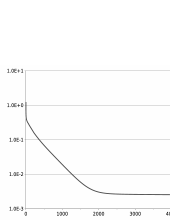
We graph the norm of , plotted on a logarithmic scale, under this procedure; for two of the cases discussed in the next Section. There is a short initial period in which the decrease is very rapid. Then there is long intermediate period where the decrease is approximately exponential, until the norm is quite close to its limiting value. After this the decrease is much slower. (We expect that the first period is that in which nonlinear effects are important and that in the second period the iteration is close to the iteration of a linear map, which in turn should be close to the linearisation of the “Calabi flow”.)
![[Uncaptioned image]](/html/0803.0987/assets/x4.png)
4 Numerical results
Suppose we have an algebraic metric which we hope to be a good approximation to an extremal metric. To compare across different values of we rescale so that the average value of is . Setting we compute three measures of the size of the “error”:
-
•
The error. That is to say, the square root of the average of .
-
•
The maximum and minimum values of .
-
•
The “maximum and minimum normalised values” of . To motivate this, consider a situation where, on average, is very small compared with the full curvature tensor. Then an error might appear large compared with the average value of , while still being small compared with the full curvature, and hence it terms of the true geometry of the manifold. More generally, we may have a situation where the curvature tensor of the manifold is much larger in some regions than others—in other words the natural scales on which to study the manifold are different in different regions. To take account of this we define the maximum and minimum normalised error to be the maximum and minimum values of , where is the pointwise norm of the full curvature tensor.
4.1 The hexagon
Recall from the introduction that this is the polygon which corresponds to the Kahler-Einstein metric on the blow-up of the projective plane at three general points. In this special case there is another, simpler, approach which one can try—the “ algorithm” described in [3], and in a separate programme we have verified numerically that this does indeed converge. But here we will just treat the manifold by our general procedure—designed for extremal metrics. See also the discussion in [8].
We find that we get a useful approximation to the Kahler-Einstein metric with the low value . The co-efficients of the refined approximation appear in the figure in Section 2.1, in the table below we record the largest and smallest of these cefficients and the “error measures”.
|
Taking larger values of we can do much better. There seems to be no practical gain in going beyond which yields:
|
In the next table we record data about the size of the components of the curvature tensor.
|
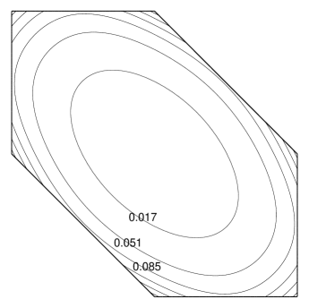
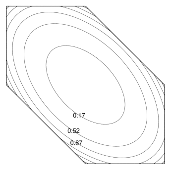
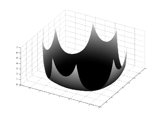
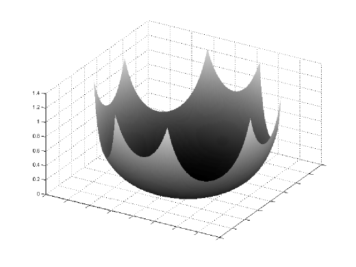
We see that the trace-free Ricci tensor is indeed very small and effectively the only non-trivial components of the curvature tensor are the “Gauss” and “Weyl” components. The Gauss curvature, times , is plotted in Figure 3. The Gauss curvature vanishes at the centre of the hexagon and is everywhere negative. (We know a priori that it has to be negative on average, since the Euler characteristic of is .) The norm of the Weyl component is plotted in Figure 4. We see that the Weyl component also vanishes at the centre of the hexagon. Recall that this Weyl component is a “-holomorphic” quartic differential on the oriented double cover of . The number of zeros, counted with multiplicity, on this double cover is . Since there are copies of making up this double cover, we can see from symmetry arguments that the only possibility is a double zero at the centre of . It is interesting to compare the curvature tensor of this manifold with those of the standard examples in (5),(6).
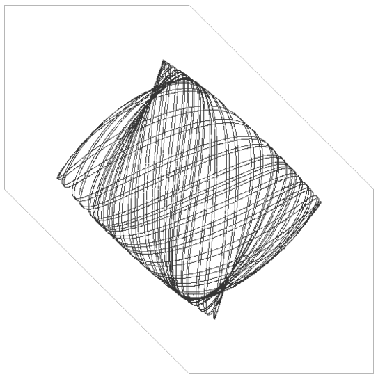
4.1.1 Geodesics
Using our numerical solutions for the Kahler-Einstein metric we can compute geodesics in this Riemannian manifold. The inner products with the two Killing fields defining the torus action are conserved quantities which we refer to as “angular momenta”. Fixing the angular momenta, the geodesic equations can be regarded as equations for a particle moving around the polygon in a potential. We do not take this any further here, and include this discussion only to demonstrate that one can effectively study the Riemannian geometry of these solutions. One could take the ideas much further. However the solutions display some interesting phenomena. When the angular momenta are reasonably large compared with the horizontal component of the velocity the solutions behave effectively as an integrable system, essentially confined to tori in the phase space. As the angular momenta are reduced the dynamics changes its nature and the solutions are more complicated. Of course, we might expect the latter from the fact that when the angular momenta are zero the equations can be viewed as the geodesic equations on the surface and since this has negative curvature the system cannot be integrable.
4.2 The pentagon
Here we discuss the pentagon, shown with , which corresponds to the blow-up of the complex projective plane at two distinct points, with the Kahler class equal to .
The metric we seek is an extremal metric but not of constant scalar curvature. The numerical results, regarding speed of convergence and the size of the errors, are very similar to those for the hexagon.
With we get
|
The curvature data is given by
|
The curvature functions are plotted in Figures 6,7,8. (In Figure 8 one can see the approximate location of a single zero of the Weyl component, as predicted by topology.)
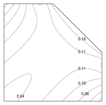
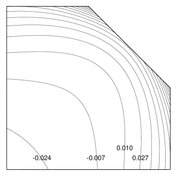
4.2.1 The conformally-Kahler Einstein metric
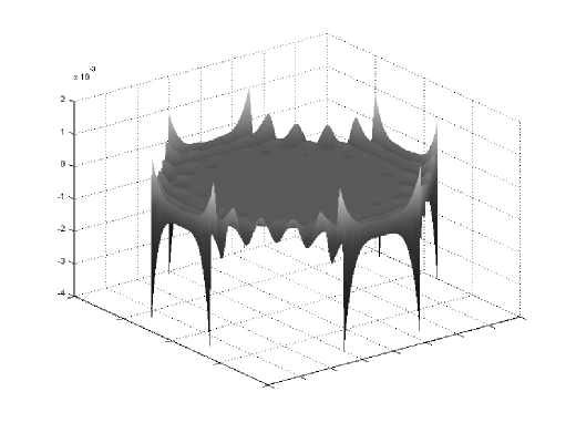
As we mentioned above, the existence of this extremal metric was proved recently by Chen, LeBrun and Weber [1]. In fact they established the existence of a family of extremal Kahler metrics on this manifold, depending on a real parameter which determines the Kahler class. The class we are considering has . Chen, LeBrun and Weber show that for a particular value the Bach tensor vanishes and the extremal metric is conformal to an Einstein metric, with conformal factor the scalar curvature. This extremal metric is not directly accessible with our method, which is confined to rational values of the parameter with fairly small denominator. However, since is close to we can expect that our extremal metric has small Bach tensor, leading to a reasonable approximation to the Einstein metric. We verify this numerically. The norm of the Bach tensor is shown in Figure 9. It is less than .005 over most of the manifold, and has maximum value about . This is comparable with , as one would expect. It would be possible to compute geometric quantities associated to the Einstein metric to this degree of accuracy.
4.3 The octagon
We now move on to the octagon depicted, which corresponds to the projective plane blow up at five points, or blown up at four points. The symmetry of the polygon shows immediately that the Futaki invriant vanishes, so the metric we seek has constant scalar curvature. The existence of this metric follows from the general result in [5]. (An argument of Zhou and Zhu [9] shows that this polygon satisfies the “positivity” criterion in the general existence theorem.)
We find that we need to take significantly larger than in the previous two cases, to get a reasonable approximate solution. Taking we obtain
|
When we get
|
The reason why we need to make larger than for the previous two polygons is clear when we look at the size of the curvature tensor:
|
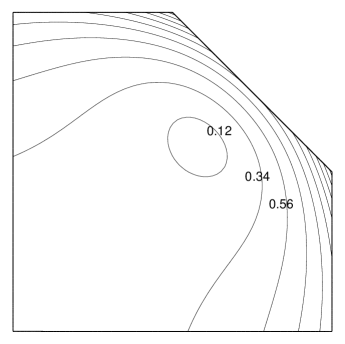
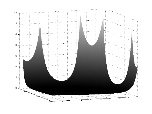
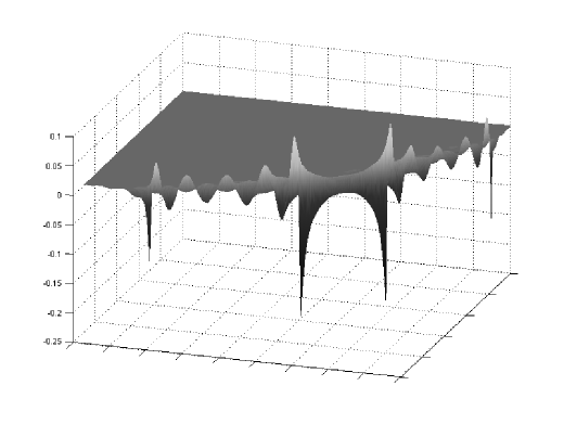
The maximum curvature in this case is nearly 3 times that for the hexagon and pentagon. Now behaves as a length-scale parameter in the asymptototic theory, and curvature scales as . So we would expect that for the octagon we should take about 3 times as large as for the pentagon or hexagon, to obtain comparable accuracy. The figures above are consistent with this. The size of the full curvature tensor and of the trace-free Ricci component are shown in Figures 10,11. Notice that the curvature is much larger near the boundary of the polygon. Moreover it is larger near edges corresponding to the curves than the curves. The Chern-Weil formula (7) shows that as the number of edges of the polygon increases the full curvature tensor grow, on average, compared to the scalar curvature. Also, the self-intersection number of a boundary sphere can be written as an integral of an expression involving the curvature over the corresponding edge, so the curvature must become relatively large there. But the actual concentration of the curvature is more dramatic than one might have expected on such general grounds.
Figure 12 shows the size of the “error” over the polygon. As we would expect the error is much larger near the boundary, where the curvature is large (which is reflected by the normalised errors in the tables above). Notice the intricate oscillatory pattern in the function, which one can see is related to the lattice spacing.
4.4 The heptagon
This is the polygon as shown (with ). It corresponds to a manifold we get by blowing up two of the fixed points in the pentagon manifold. The self-intersection numbers are as shown, and there is one curve.
The metric we seek is an extremal metric, not of constant scalar curvature. The results follow a similar pattern to the previous case, only more so. We take (which is about as large as seems reasonable with the programme), and we obtain:
|
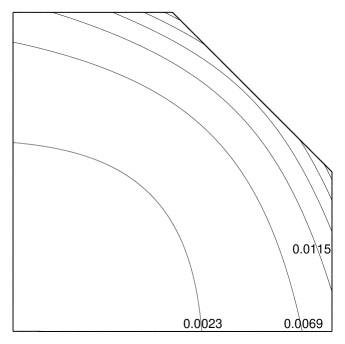
The error is concentrated near the boundary and particularly near the curve, which is where the curvature is largest. The modulus of the minimum value looks large, and one might think that the approximation is not very satisfactory, but the normalised value is much smaller. Thus we believe that this does model an exact solution quite well. The maximum value of the curvature is nearly 6 times that for the hexagon, so we should expect to achieve an accuracy similar to that for the hexagon with , and the results are in line with this. Notice that the curvature function in Figure 13 is almost constant, at a value about , over most of the polygon.
|
5 Conclusions
-
•
Rate of convergence
As we have stated in Section 3, one can expect that the refined approximations converge to the extremal metric faster than any inverse power. But, even if proved rigorously, this is only an asymptotic statement and does not give any information about particular values of . To examine this experimentally, we consider the error as a measure of the distance to the true solution, working with the hexagon, over a range of different values of :
4 6 8 10 12 16 20 Error .019 .0077 .0012 .00052 .00010 The data fits reasonably well with an exponential decrease .
-
•
Speed and size of the calculation For a fixed “shape” of polygon the number of elementary calculations required in each step of the iteration is proportional to , since we have to evaluate functions, and their derivatives at points. In the more general case of a -dimensional toric variety this would be . As increases we need to increase , since the functions we are integrating become increasingly localised. Simple asymptotics suggests that one should take , so the number of elementary calculations is . However, at a given point, most of the functions are extremely small, so one can hope to reduce the calculation by ignoring them. This idea was implemented to some extent in our programme, which “truncates” the sums to ignore the very small terms. This does not affect the accuracy noticeably but the gain we have achieved so far is only modest. With a more sophisticated approach, one could hope to make substantial gains, particularly when is large, or in higher dimensional problems. Simple asymptotics suggests that one might be able to reduce the calculation at each point to , giving for each iteration step.
The convergence is also slower as increases. One expects that the number of steps required to effectively reach a fixed point will be . (For example, in Figure 2 the number of steps to reach the marked “corner” in the graph for the pentagon, with , is about , while for the heptagon, with , it takes about steps: then .) So in sum we can hope that the length of time needed to run the whole procedure, in dimension , will be without the truncation of the sums described above, and perhaps , with this truncation.
-
•
Scope for improvement
The most striking feature of our results is the extent to which the curvature of the solutions becomes concentrated around the boundary of the polygon or, in terms of the -manifolds, around the exceptional curves. This is particularly true of the curves with large negative self-intersection. The obvious way to handle this efficiently would be to adopt a “multiscale” technique. This idea can be related to the “Veronese embedding” in algebraic geometry, as discussed in [4]. Suppose we have an algebraic metric defined by an array of coefficients , for a certain lattice-size . The Kahler potential is . Then we can write
We can expand out the sum to write
where
This means that, after rescaling, we can obtain the same metric using the array but with lattice scale . Now suppose we have chosen a subset . Then we can consider varying our array to
where is zero if is not in . The potential function is
If the number of elements of is relatively small then we can calculate this function and its derivatives relatively quickly. But if we choose appropriately we can hope to get a much more accurate approximation to the true metric over the high curvature regions. For example in the case of the heptagon we might take , which should suffice to describe the metric over the interior of the polygon, and a set consisting of lattice points near to the boundary, so that we would effectively be approximating the metrics in that region as though we were working with .
Of course we can imagine iterating this construction to a yet larger lattice scale , and so on. Also, there is nothing special about the factor . But what is needed to develop this approach is to find some reliable algorithms for updating the different coefficients.
References
- [1] Chen, X., LeBrun, C. and Weber,B. On conformally Kahler, Einstein manifolds Arxiv DG/ 07050710
- [2] Donaldson, S. K. Scalar curvature and stability of toric varieties Jour. Differential Geometry 62 (2002) 289-349
- [3] Donaldson, S. K. Some numerical results in complex differential geometry Arxiv DG/0512625 To appear in Quarterly Journal of Pure and Applied Mathematics.
- [4] Donaldson,S.K. Kahler Geometry on toric manifolds, and some other manifolds with large symmetry
- [5] Donaldson,S.K. Constant scalar curvature metrics on toric surfaces In preparation.
- [6] Doran, C. Headrick,M.,Herzog,C.P.,Kantor, J., Wiseman, T. Numerical Kahler-Einstein metric on the third del Pezzo hep-th/0703057
- [7] Douglas, M.R., Karp,R.L., Lukic,S. and Reinbacher,R. Numerical Calabi-Yau metrics hep-th/0612075
- [8] Keller,J. Ricci iterations on Kahler classes arxiv:math DG/07091490
- [9] Zhou,B. and Zhu,X. Relative K-stability and modified K-energy on toric manifolds arxiv:math.DG/06032337