New Probabilistic Interest Measures for Association Rules

Abstract

Mining association rules is an important technique for discovering meaningful patterns in transaction databases. Many different measures of interestingness have been proposed for association rules. However, these measures fail to take the probabilistic properties of the mined data into account. We start this paper with presenting a simple probabilistic framework for transaction data which can be used to simulate transaction data when no associations are present. We use such data and a real-world database from a grocery outlet to explore the behavior of confidence and lift, two popular interest measures used for rule mining. The results show that confidence is systematically influenced by the frequency of the items in the left hand side of rules and that lift performs poorly to filter random noise in transaction data. Based on the probabilistic framework we develop two new interest measures, hyper-lift and hyper-confidence, which can be used to filter or order mined association rules. The new measures show significantly better performance than lift for applications where spurious rules are problematic.

Keywords:

Data mining, association rules, measures of interestingness, probabilistic data modeling.

1 Introduction

Mining association rules [3] is an important technique for discovering meaningful patterns in transaction databases. An association rule is a rule of the form $X\Rightarrow Y$, where $X$ and $Y$ are two disjoint sets of items (itemsets). The rule means that if we find all items in $X$ in a transaction it is likely that the transaction also contains the items in $Y$.

Association rules are selected from the set of all possible rules using measures of significance and interestingness. Support, the primary measure of significance, is defined as the fraction of transactions in the database which contain all items in a specific rule [3]. That is,

$$\mathrm{supp}(X\Rightarrow Y)=\mathrm{supp}(X\cup Y)=\frac{c_{XY}}{m},$$ (1)

where $c_{XY}$ represents the number of transactions which contain all items in $X$ and $Y$, and $m$ is the number of transactions in the database.

For association rules, a minimum support threshold is used to select the most frequent (and hopefully important) item combinations called frequent itemsets. The process of finding these frequent itemsets in a large database is computationally very expensive since it involves searching a lattice which, in the worst case, grows exponentially in the number of items. In the last decade, research has centered on solving this problem and a variety of algorithms were introduced which render search feasible by exploiting various properties of the lattice (see [14] for pointers to the currently fastest algorithms).

From the frequent itemsets all rules which satisfy a threshold on a certain measures of interestingness are generated. For association rules, Agrawal et al. [3] suggest using a threshold on confidence, one of many proposed measures of interestingness. A practical problem is that with support and confidence often too many association rules are produced. One possible solution is to use additional interest measures, such as e.g. lift [9], to further filter or rank found rules.

Several authors [9, 2, 27, 1] constructed examples to show that in some cases the use of confidence and lift can be problematic. Here, we instead take a look at how pronounced and how important such problems are when mining association rules. To do this, we visually compare the behavior of support, confidence and lift on a transaction database from a grocery outlet with a simulated data set which only contain random noise. The data set is simulated using a simple probabilistic framework for transaction data (first presented by Hahsler et al. [17]) which is based on independent Bernoulli trials and represents a null model with “no structure.”

Based on the probabilistic approach used in the framework, we will develop and analyze two new measures of interestingness, hyper-lift and hyper-confidence. We will show how these measures are better suited to deal with random noise and that the measures do not suffer from the problems of confidence and lift.

This paper is structured as follows: In Section 2, we introduce the probabilistic framework for transaction data. In Section 3, we apply the framework to simulate a comparable data set which is free of associations and compare the behavior of the measures confidence and lift on the original and the simulated data. Two new interest measures are developed in Section 4 and compared on three different data sets with lift. We conclude the paper with the main findings and a discussion of directions for further research.

An implementation of the probabilistic framework and the new measures of interestingness proposed in this paper is included in the freely available R extension package arules [16].

2 A simple probabilistic framework for transaction data

Figure 1: Transactions occurring over time following a Poisson process.

A transaction database consists of a series of transactions, each transaction containing a subset of the available items. We consider transactions which are recorded during a fixed time interval of length $t$. In Figure 1 an example time interval is shown as an arrow with markings at the points in time when the transactions denoted by $\mathit{Tr}_{1}$ to $\mathit{Tr}_{m}$ occur. For the model we assume that transactions occur randomly following a (homogeneous) Poisson process with parameter $\theta$. The number of transactions $m$ in time interval $t$ is then Poisson distributed with parameter $\theta t$ where $\theta$ is the intensity with which transactions occur during the observed time interval:

$$P(M=m)=\frac{e^{-\theta t}(\theta t)^{m}}{m!}$$ (2)

We denote the items which occur in the database by $L=\{l_{1},l_{2},\ldots,l_{n}\}$ with $n$ being the number of different items. For the simple framework we assume that all items occur independently of each other and that for each item $l_{i}\in L$ there exists a fixed probability $p_{i}$ of being contained in a transaction. Each transaction is then the result of $n$ independent Bernoulli trials, one for each item with success probabilities given by the vector $p=(p_{1},p_{2},\dots,p_{n})$. Table 1 contains the typical representation of an example database as a binary incidence matrix with one column for each item. Each row labeled $\mathit{Tr}_{1}$ to $\mathit{Tr}_{m}$ contains a transaction, where a 1 indicates presence and a 0 indicates absence of the corresponding item in the transaction. Additionally, in Table 1 the success probability for each item is given in the row labeled $p$ and the row labeled $c$ contains the number of transactions each item is contained in (sum of the ones per column).

	items
transactions	$l_{1}$	$l_{2}$	$l_{3}$	…	$l_{n}$
$Tr_{1}$	$0$	$1$	$0$	…	$1$
$Tr_{2}$	$0$	$1$	$0$	…	$1$
$Tr_{3}$	$0$	$1$	$0$	…	$0$
$Tr_{4}$	$0$	$0$	$0$	…	$0$
$\vdots$	$\vdots$	$\vdots$	$\vdots$	$\ddots$	$\vdots$
$Tr_{m-1}$	$1$	$0$	$0$	…	$1$
$Tr_{m}$	$0$	$0$	$1$	…	$1$
$c$	$99$	$201$	$7$	…	$411$
$p$	$0.005$	$0.01$	$0.0003$	…	$0.025$

Table 1: Example transaction database with transaction counts per item $c$ and items success probabilities $p$.

Following the model, $c_{i}$, the observed number of transactions item $l_{i}$ is contained in, can be interpreted as a realization of a random variable $C_{i}$. Under the condition of a fixed number of transactions $m$, this random variable has the following binomial distribution.

$$P(C_{i}=c_{i}|M=m)=\binom{m}{c_{i}}p_{i}^{c_{i}}(1-p_{i})^{m-c_{i}}$$ (3)

However, since for a given time interval the number of transactions is not fixed, the unconditional distribution gives:

$$\begin{split}P(C_{i}=c_{i})&=\sum_{m=c_{i}}^{\infty}P(C_{i}=c_{i}|M=m)\cdot P(M=m)\\ &=\sum_{m=c_{i}}^{\infty}\binom{m}{c_{i}}p_{i}^{c_{i}}(1-p_{i})^{m-c_{i}}\;\frac{e^{-\theta t}(\theta t)^{m}}{m!}\\ &=\frac{e^{-\theta t}(p_{i}\theta t)^{c_{i}}}{c_{i}!}\sum_{m=c_{i}}^{\infty}\frac{((1-p_{i})\theta t)^{m-c_{i}}}{(m-c_{i})!}\\ &=\frac{e^{-p_{i}\theta t}(p_{i}\theta t)^{c_{i}}}{c_{i}!}.\\ \end{split}$$ (4)

The term $\sum_{m=c_{i}}^{\infty}\frac{((1-p_{i})\theta t)^{m-c_{i}}}{(m-c_{i})!}$ in the second to last line in Equation LABEL:eq:prob is an exponential series with sum $e^{(1-p_{i})\theta t}$. After substitution we see that the unconditional probability distribution of each $C_{i}$ follows a Poisson distribution with parameter $p_{i}\theta t$. For short we will use $\lambda_{i}=p_{i}\theta t$ and introduce the parameter vector $\lambda=(\lambda_{1},\lambda_{2},\dots,\lambda_{n})$ of the Poisson distributions for all items. This parameter vector can be calculated from the success probability vector $p$ and vice versa by the linear relationship $\lambda=p\theta t$.

For a given database, the values of the parameter $\theta$ and the success vectors $p$ or alternatively $\lambda$ are unknown but can be estimated from the database. The best estimate for $\theta$ from a single database is $m/t$. The simplest estimate for $\lambda$ is to use the observed counts $c_{i}$ for each item. However, this is only a very rough estimate which gets especially unreliable for small counts. There exist more sophisticated estimation approaches. For example, DuMouchel and Pregibon [11] use the assumption that the parameters of the count processes for items in a database are distributed according to a continuous parametric density function. This additional information can improve estimates over using just the observed counts.

Alternatively, the parameter vector $p$ can be drawn from a parametric distribution. A suitable distribution is the Gamma distribution which is very flexible and allows to fit a wide range of empirical data. A Gamma distribution together with the independence model introduced above is known as the Poisson-Gamma mixture model which results in a negative binomial distribution and has applications in many fields [21]. In conjunction with association rules this mixture model was used by Hahsler [15] to develop a model-based support constraint.

Independence models similar to the probabilistic framework employed in this paper have been used for other applications. In the context of query approximation, where the aim is to predict the results of a query without scanning the whole database, Pavlov et al. [24] investigated the independence model as an extremely parsimonious model. However, the quality of the approximation can be poor if the independence assumption is violated significantly by the data.

Cadez et al. [10] and Hollmén et al. [19] used the independence model to cluster transaction data by learning the components of a mixture of independence models. In the former paper the aim is to identify typical customer profiles from market basket data for outlier detection, customer ranking and visualization. The later paper focuses on approximating the joint probability distribution over all items by mining frequent itemsets in each component of the mixture model, using the maximum entropy technique to obtain local models for the components, and then combining the local models.

Almost all authors use the independence model to learn something from the data. However, the model only uses the marginal probabilities $p$ of the items and ignores all interactions. Therefore, the accuracy and usefulness of the independence model for such applications is drastically limited and models which incorporate pair-wise or even higher interactions provide better results. For the application in this paper, we explicitly want to generate data with independent items to evaluate measures of interestingness.

3 Simulated and real-world database

We use 1 month ($t=30$ days) of real-world point-of-sale transaction data from a typical local grocery outlet. For convenience reasons we use categories (e.g., popcorn) instead of the individual brands. In the available $m=9835$ transactions we found $n=169$ different categories for which articles were purchased. This database is called “Grocery” and is freely distributed with the R extension package arules [16].

The estimated transaction intensity $\theta$ for Grocery is $m/t=327.5$ transactions per day. To simulate comparable data using the framework, we use the Poisson distribution with the parameter $\theta t$ to draw the number of transactions $m$ (9715 in this experiment). For simplicity we use the relative observed item frequencies as estimates for $\lambda$ and calculate the success probability vector $p$ by $\lambda/\theta t$. With this information we simulate the $m$ transactions in the transaction database. Note, that the simulated database does not contain any associations (all items are independent), and thus differs from the Grocery database which is expected to contain associations. In the following we will use the simulated data set not to compare it to the real-world data set, but to show that interest measures used for association rules exhibit similar effects on real-world data as on simulated data without any associations.

For the rest of this section we concentrate on $2$-itemsets, i.e., the co-occurrences between two items denoted by $l_{i}$ and $l_{j}$ with $i,j=1,2,\dots,n$ and $i\neq j$. Although itemsets and rules of arbitrary length can be analyzed using the framework, we restrict the analysis to $2$-itemsets since interest measures for these associations are easily visualized using 3D plots. In these plots the $x$ and $y$-axis each represent the items $l_{i}$ and $l_{j}$ ordered from the most frequent to the least frequent from left to right and front to back. On the $z$-axis we plot the analyzed measure.

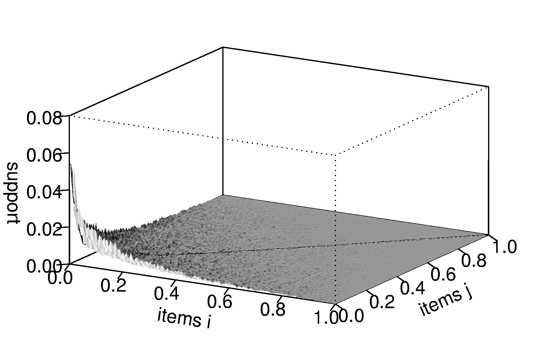
(a) simulated

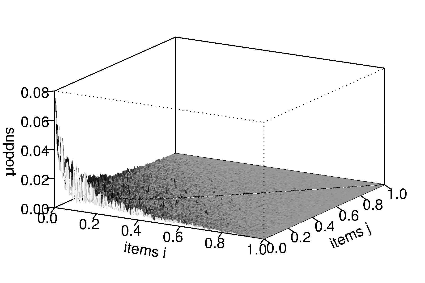
(b) Grocery

Figure 2: Support distributions of all $2$-itemsets (items are ordered by decreasing support from left to right and front to back).

First we compare the $2$-itemset support. Figure 2 shows the support distribution of all $2$-itemsets. Naturally, the most frequent items also form together the most frequent itemsets (to the left in the front of the plots). The general forms of the two support distributions in the plot are very similar. The Grocery data set reaches higher support values with a median of $0.000203$ compared to $0.000113$ for the simulated data. This indicates that the Grocery data set contains associated items which co-occur more often than expected under independence.

3.1 The interest measure confidence

Confidence is defined by Agrawal et al. [3] as

$$\mathrm{conf}(X\Rightarrow Y)=\frac{\mathrm{supp}(X\cup Y)}{\mathrm{supp}(X)},$$ (5)

where $X$ and $Y$ are two disjoint itemsets. Often confidence is understood as an estimate of the conditional probability $P(E_{Y}|E_{X})$, were $E_{X}$ ($E_{Y}$) is the event that $X$ ($Y$) occurs in a transaction [18].

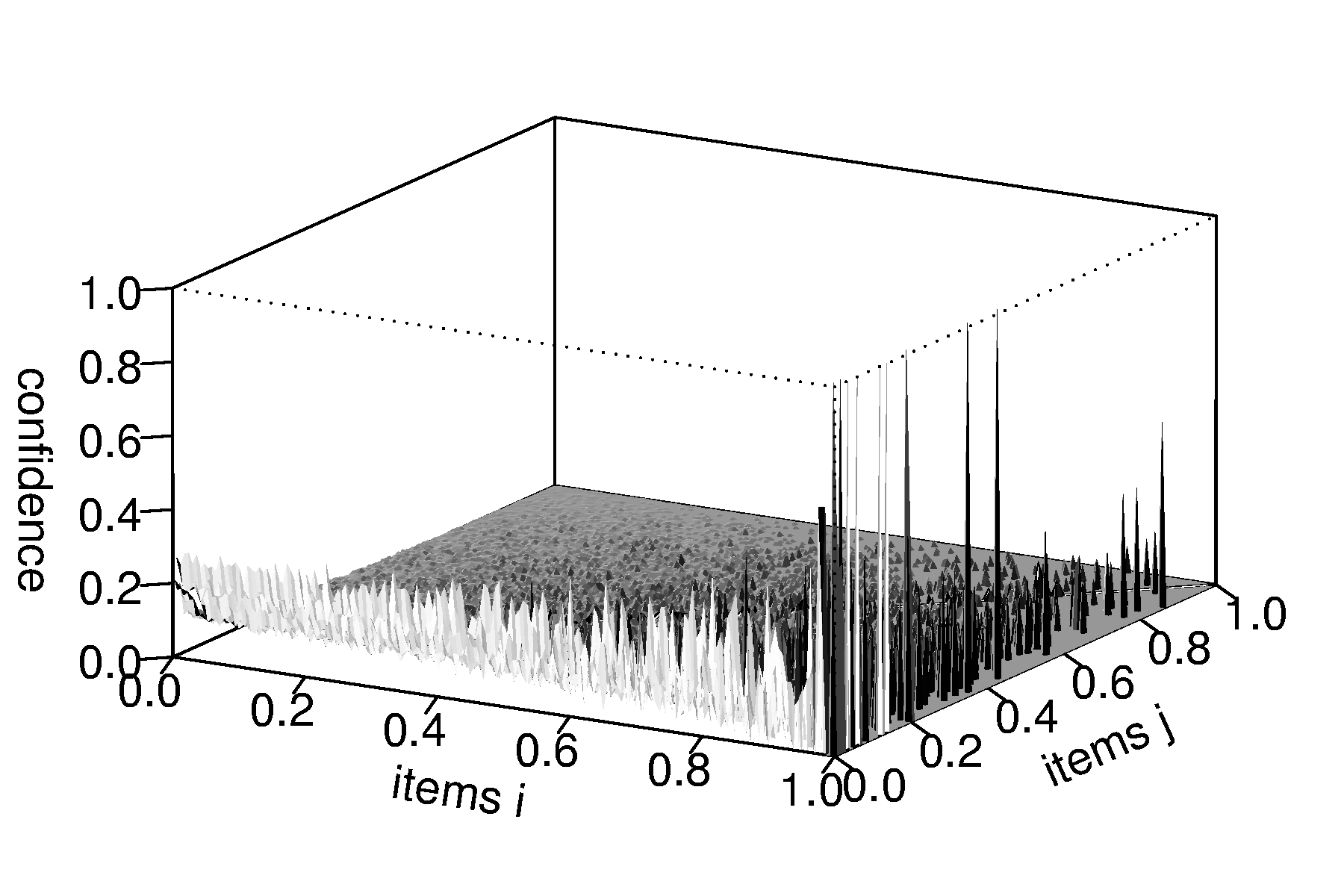
(a) simulated

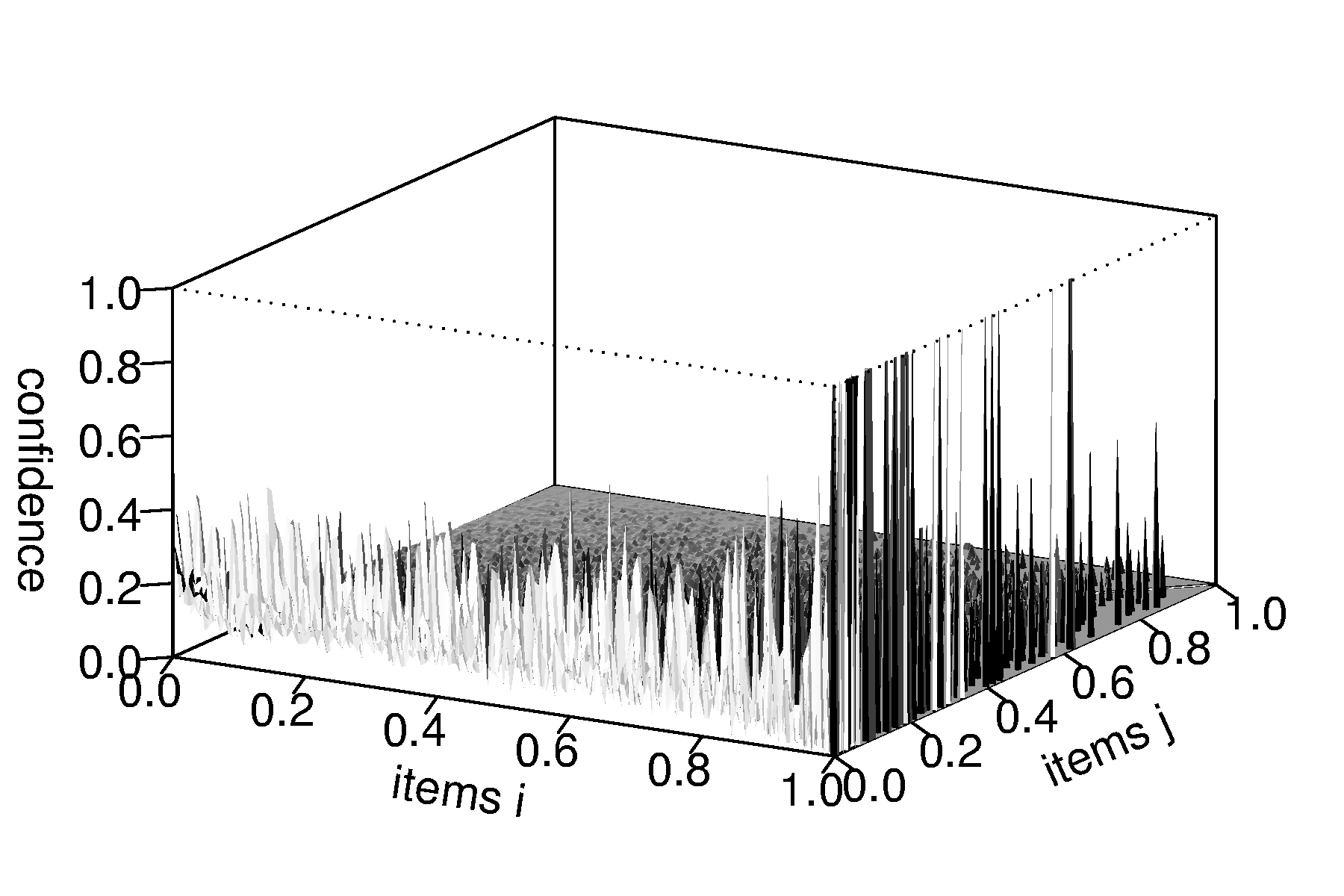
(b) Grocery

Figure 3: Confidence distributions of all rules containing 2 items.

From the $2$-itemsets we generate all rules of the from $l_{i}\Rightarrow l_{j}$ and present the confidence distributions in Figures 3. Confidence is generally much lower for the simulated data (with a median of $0.0086$ to $0.0140$ for the real-world data). Finding higher confidence values in the real-world data, which are expected to contain associations, indicates that the confidence measure is able to suppress noise. However, the plots in Figure 3 also show that confidence always increases with the item in the right hand side of the rule ($l_{j}$) getting more frequent. This behavior directly follows from the way confidence is calculated. If the frequency of the right hand side of the rule increases, confidence will increase even if the items in the rule are not related (see itemset $Y$ in Equation 5). For the Grocery data set in Figure 3(b) we see that this effect dominates the confidence measure. The fact that confidence clearly favors some rules makes the measure problematic when it comes to selecting or ranking rules.

3.2 The interest measure lift

Typically, rules mined using minimum support (and confidence) are filtered or ordered using their lift value. The measure lift (also called interest [9]) is defined on rules of the form $X\Rightarrow Y$ as

$$\mathrm{lift}(X\Rightarrow Y)=\frac{\mathrm{conf}(X\Rightarrow Y)}{\mathrm{supp}(Y)}.$$ (6)

A lift value of $1$ indicates that the items are co-occurring in the database as expected under independence. Values greater than one indicate that the items are associated. For marketing applications it is generally argued that $\mathrm{lift}>1$ indicates complementary products and $\mathrm{lift}<1$ indicates substitutes [6, 20].

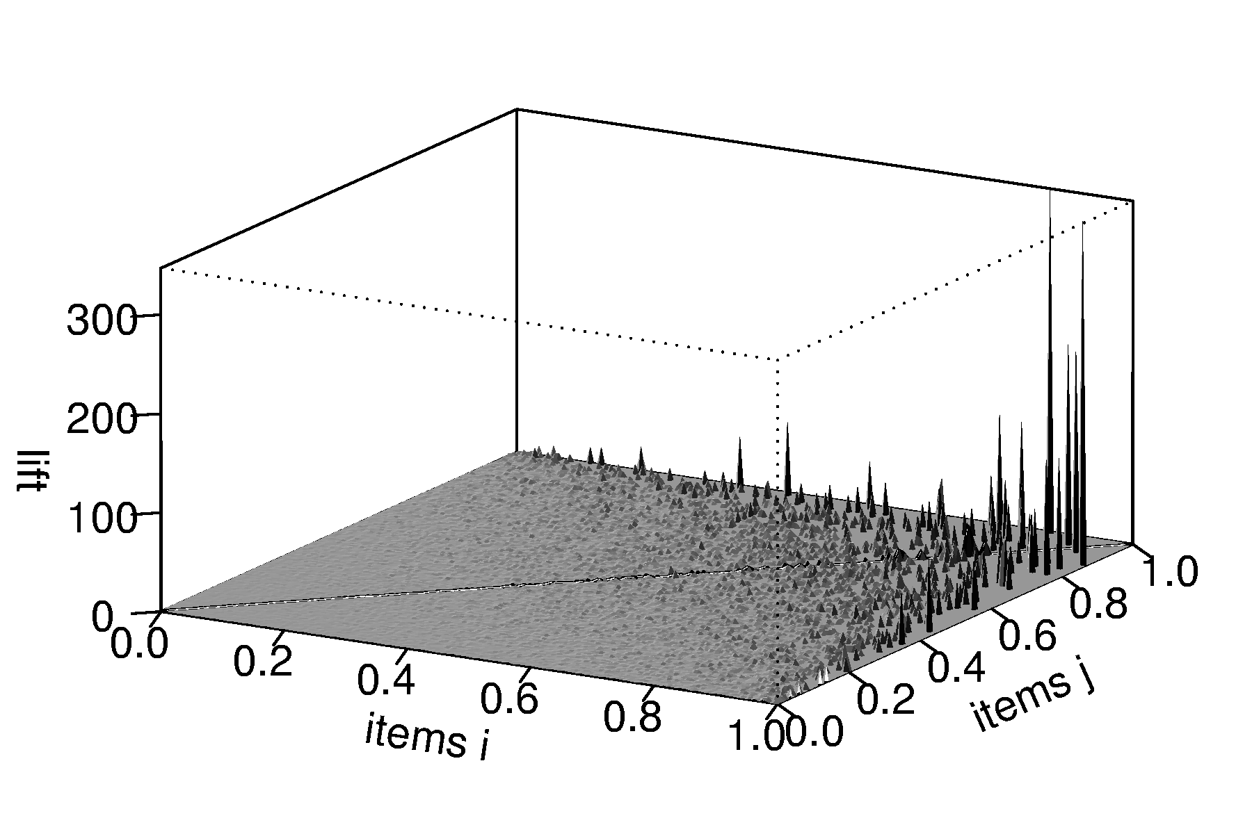
(a) simulated

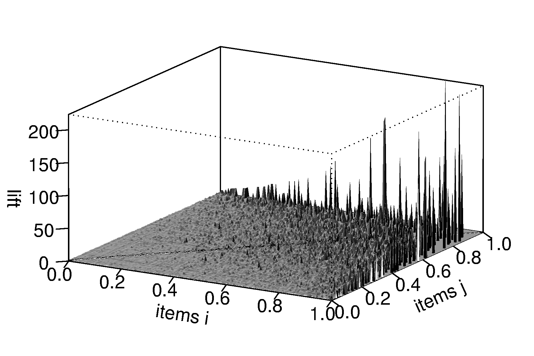
(b) Grocery

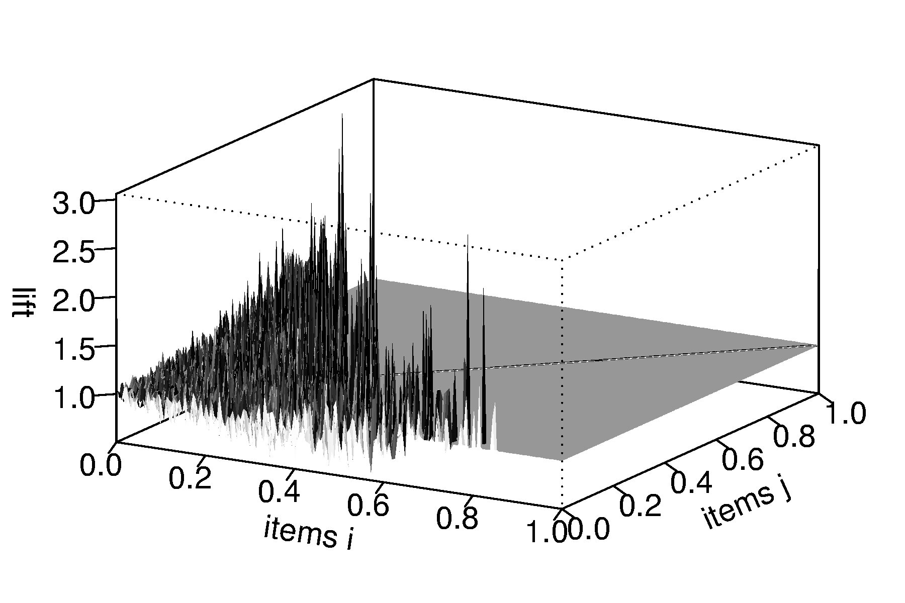
(c) simulated with $\mathrm{supp}>0.1\%$

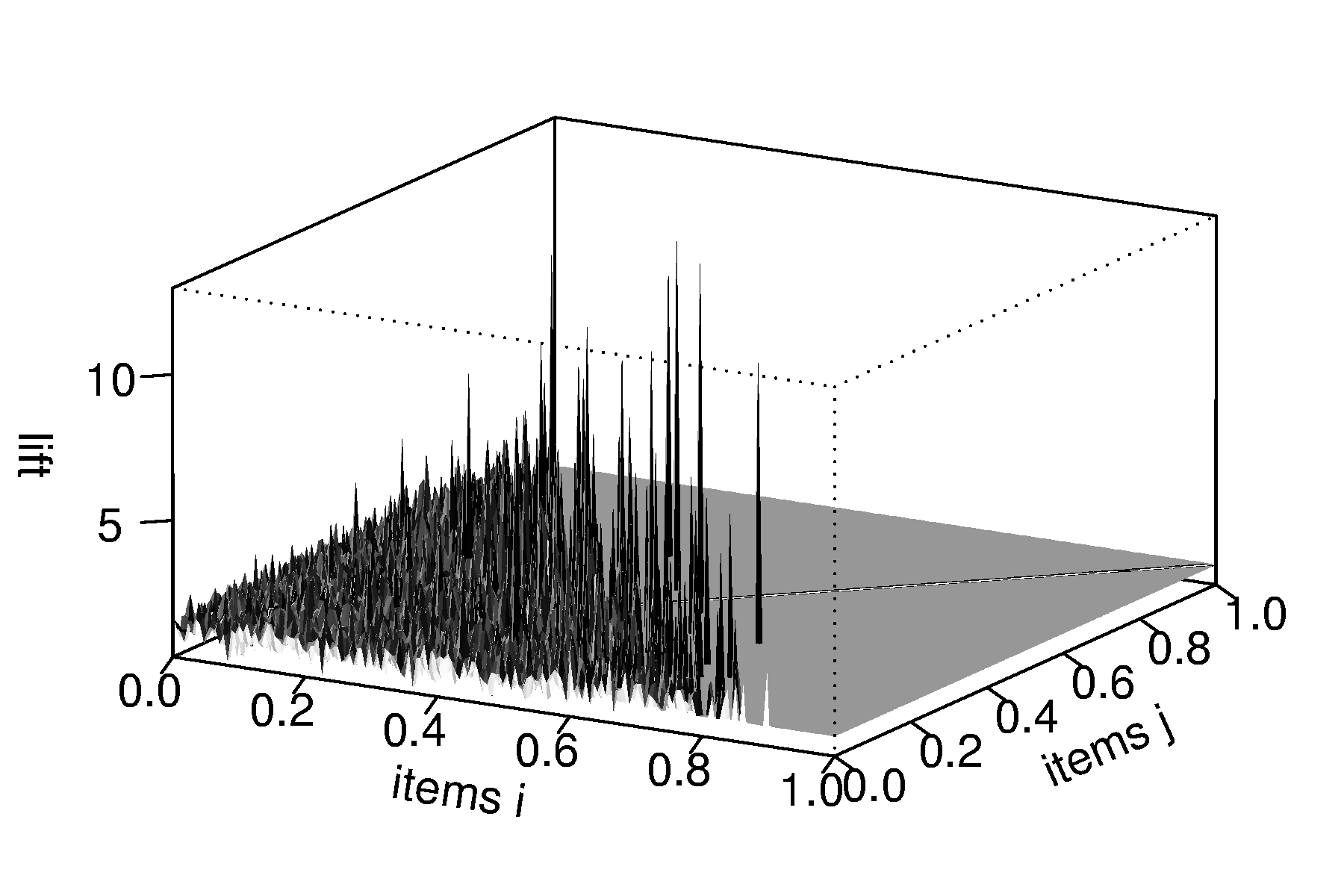
(d) Grocery with $\mathrm{supp}>0.1\%$

Figure 4: Lift distributions of all rules with two items.

Figure 4 show the lift values for the two data sets. The general distribution is again very similar. In the plots in Figures 4(a) and 4(b) we can only see that very infrequent items produce extremely high lift values. These values are artifacts occurring when two very rare items co-occur once together by chance. Such artifacts are usually avoided in association rule mining by using a minimum support on itemsets. In Figures 4(c) and 4(d) we applied a minimum support of 0.1%. The plots show that there exist rules with higher lift values in the Grocery data set than in the simulated data. However, in the simulated data we still find 50 rules with a lift greater than 2. This indicates that the lift measure performs poorly to filter random noise in transaction data especially if we are also interested in relatively rare items with low support. The plots in Figures 4(c) and 4(d) also clearly show lift’s tendency to produce higher values for rules containing less frequent items resulting in that the highest lift values always occur close to the boundary of the selected minimum support. We refer the reader to [5] for a theoretical treatment of this effect. If lift is used to rank discovered rules this means that there is not only a systematic tendency towards favoring rules with less frequent items but the rules with the highest lift will also always change with even small variations of the user-specified minimum support.

4 New measures of interest

In the simple probabilistic model all items as well as combinations of items occur following independent Poisson processes. If we look at the observed co-occurrence counts of all pairs of two items, $l_{i}$ and $l_{j}$, in a data set with $m$ transactions, we can form an $n\times n$ contingency table. Each cell can be modeled by a random variable $C_{ij}$ which, given fixed marginal counts $c_{i}$ and $c_{j}$, follows a hyper-geometric distribution.

The hyper-geometric distribution arises for the so-called urn problem, where the urn contains $w$ white balls and $b$ black balls. The number of white balls drawn with $k$ trials without replacement follows a hyper-geometric distribution. This model is applicable for counting co-occurrences for independent items $l_{i}$ and $l_{j}$ in the following way: Item $l_{j}$ occurs in $c_{j}$ transactions, therefore, we can represent the database as an urn which contains $c_{j}$ transactions with $l_{j}$ (white balls) and $m-c_{j}$ transactions without $l_{j}$ (black balls). To assign item $l_{i}\neq l_{j}$ randomly to $c_{i}$ transactions, we draw without replacement $c_{i}$ transactions from the urn. The number of drawn transactions which we assign item $l_{j}$ to (and thus represent the co-occurrences between $l_{i}$ and $l_{j}$) then has a hyper-geometric distribution.

It is straightforward to extend this reasoning from two items to two itemsets $X$ and $Y$. In this case the random variable $C_{XY}$ follows a hyper-geometric distribution with the counts of the itemsets as its parameter. Formally, the probability of counting exactly $r$ transactions which contain the two independent itemsets $X$ and $Y$ is given by

$$P(C_{XY}=r)=\frac{\binom{c_{Y}}{r}\binom{m-c_{Y}}{c_{X}-r}}{\binom{m}{c_{X}}}.$$ (7)

Note that this probability is conditional to the marginal counts $c_{X}$ and $c_{Y}$. To simplify the notation, we will omit this condition also in the rest of the paper.

The probability of counting more than $r$ transactions is

$$P(C_{XY}>r)=1-\sum^{r}_{i=0}P(C_{XY}=i).$$ (8)

Based on this probability, we will develop the probabilistic measures hyper-lift and hyper-confidence in the rest of this section. Both measures quantify the deviation of the data from the independence model. This idea is a similar to the use of random data to assess the significance of found clusters in cluster analysis (see, e.g., [7]).

4.1 Hyper-lift

The expected value of a random variable $C$ with a hyper-geometric distribution is

$$E(C)=\frac{kw}{w+b},$$ (9)

where the parameter $k$ represents the number of trials, $w$ is the number of white balls, and $b$ is the number of black balls. Applied to co-occurrence counts for the two itemsets $X$ and $Y$ in a transaction database this gives

$$E(C_{XY})=\frac{c_{X}c_{Y}}{m},$$ (10)

where $m$ is the number of transactions in the database. By using Equation 10 and the relationship between absolute counts and support, lift can be rewritten as

$$\mathrm{lift}(X\Rightarrow Y)=\frac{\mathrm{conf}(X\Rightarrow Y)}{\mathrm{supp}(Y)}=\frac{\mathrm{supp}(X\cup Y)}{\mathrm{supp}(X)\ \mathrm{supp}(Y)}=\frac{c_{XY}}{E(C_{XY})}.$$ (11)

For items with a relatively high occurrence frequency, using the expected value for lift works well. However, for relatively infrequent items, which are the majority in most transaction databases and very common in other domains [28], using the ratio of the observed count to the expected value is problematic. For example, let us assume that we have the two independent itemsets $X$ and $Y$, and both itemsets have a support of 1% in a database with 10000 transactions. Using Equation 10, the expected count $E(C_{XY})$ is 1. However, for the two independent itemsets there is a $P(C_{XY}>1)$ of 0.264 (using the hyper-geometric distribution from Equation 8). Therefore there is a substantial chance that we will see a lift value of $2,3$ or even higher. Given the huge number of itemsets and rules generated by combining items (especially when also considering itemsets containing more than two items), this is very problematic. Using larger databases with more transactions reduces the problem. However, it is not always possible to obtain a consistent database of sufficient size. Large databases are usually collected over a long period of time and thus may contain outdated information. For example, in a supermarket the articles offered may have changed or shopping behavior may have changed due to seasonal changes.

To address the problem, one can quantify the deviation of the observed co-occurrence count $c_{XY}$ from the independence model by dividing it by a different location parameter of the underlying hyper-geometric distribution than the mean which is used for lift. For hyper-lift we suggest to use the quantile of the distribution denoted by $Q_{\delta}(C_{XY})$. Formally, the minimal value of the $\delta$ quantile of the distribution of $C_{XY}$ is defined by the following inequalities:

$$P(C_{XY}<Q_{\delta}(C_{XY}))\leq\delta\quad\text{and}\quad P(C_{XY}>Q_{\delta}(C_{XY}))\leq 1-\delta.$$ (12)

The resulting measure, which we call hyper-lift, is defined as

$$\mathrm{hyper\mbox{-}lift_{\delta}}(X\Rightarrow Y)=\frac{c_{XY}}{Q_{\delta}(C_{XY})}.$$ (13)

In the following, we will use $\delta=0.99$ which results in hyper-lift being more conservative compared to lift. The measure can be interpreted as the number of times the observed co-occurrence count $c_{XY}$ is higher than the highest count we expect at most 99% of the time. This means, that hyper-lift for a rule with independent items will exceed 1 only in 1% of the cases.

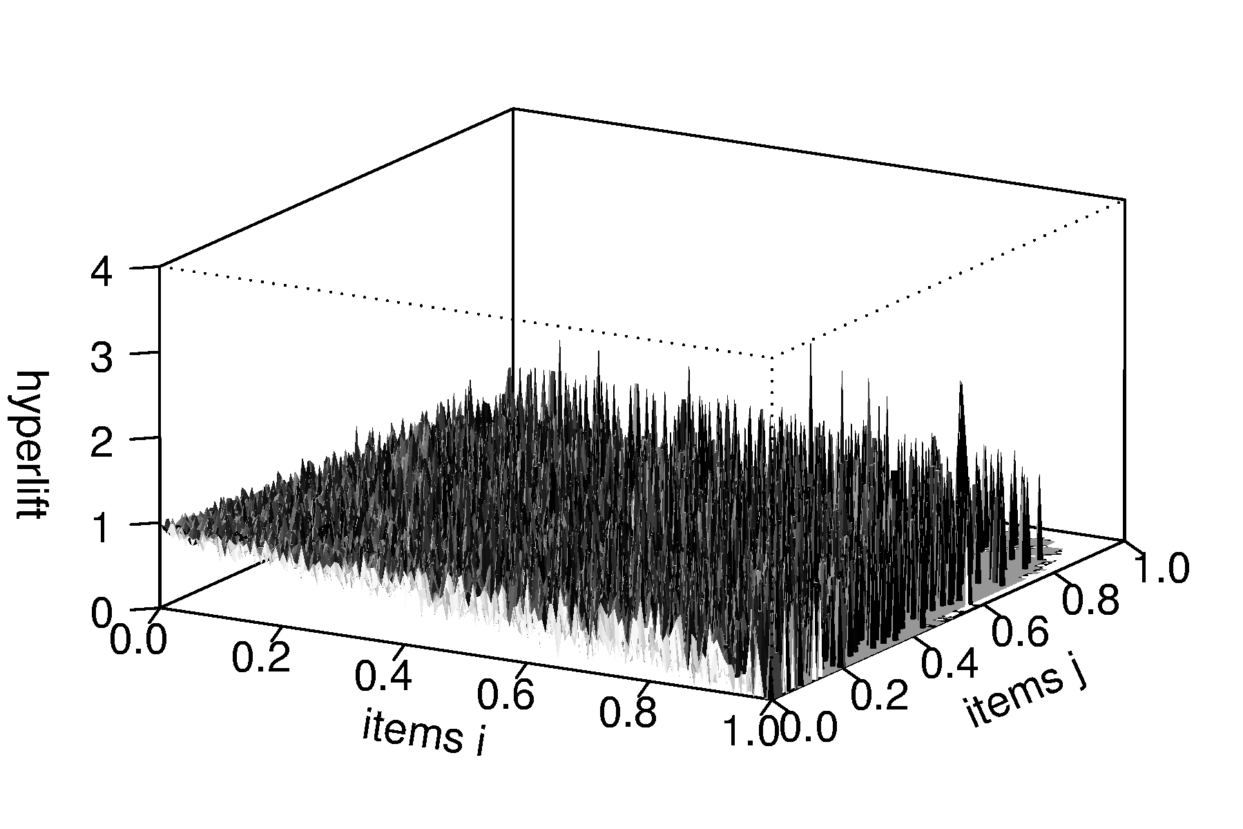
(a) simulated

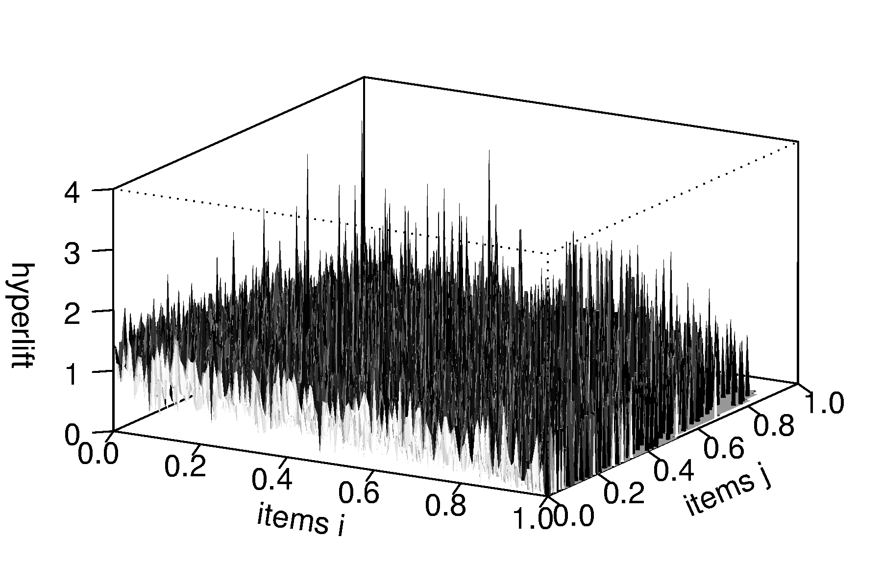
(b) Grocery

Figure 5: Hyper-lift for rules with two items.

In Figure 5 we compare the distribution of the hyper-lift values for all rules with two items at $\delta=0.99$ for the simulated and the Grocery database. Figure 5(a) shows that the hyper-lift on the simulated data is more evenly distributed than lift (compare to Figure 4 in Section 3.2). Also only for 100 of the $n\times n=28561$ rules hyper-lift exceeds 1 and no rule exceeds 2. This indicates that hyper-lift filters the random co-occurrences better than lift with 3718 rules having a lift greater than 1 and 82 rules exceed a lift of 2. However, hyper-lift also shows a systematic dependency on the occurrence probability of items leading to smaller and more volatile values for rules with less frequent items.

On the Grocery database in Figure 5(b) we find larger hyper-lift values of up to 4.286. This indicates that the Grocery database indeed contains dependencies. The highest values are observed between items with intermediate support (located closer to the center of the plot). Therefore, hyper-lift avoids lift’s problem of producing the highest values always only close to the minimum support boundary (compare Section 3.2).

Further evaluations of hyper-lift with rules including an arbitrary number of items will be presented in Section 4.3.

4.2 Hyper-confidence

Instead of looking at quantiles of the hyper-geometric distribution to form a lift-like measure, we can also directly calculate the probability of realizing a count smaller than the observed co-occurrence count $c_{XY}$ given the marginal counts $c_{X}$ and $c_{Y}$.

$$P(C_{XY}<c_{XY})=\sum_{i=0}^{c_{XY}-1}P(C_{XY}=i),$$ (14)

where $P(C_{XY}=i)$ is calculated using Equation 7 above. A high probability indicates that observing $c_{XY}$ under independence is rather unlikely. The probability can be directly used as the interest measure hyper-confidence:

$$\mathrm{hyper\mbox{-}confidence}(X\Rightarrow Y)=P(C_{XY}<c_{XY})$$ (15)

Analogously to other measures of interest, we can use a threshold $\gamma$ on hyper-confidence to accept only rules for which the probability to observe such a high co-occurrence count by chance is smaller or equal than $1-\gamma$. For example, if we use $\gamma=0.99$, for each accepted rule, there is only a 1% chance that the observed co-occurrence count arose by pure chance. Formally, using a threshold on hyper-confidence for the rules $X\Rightarrow Y$ (or $Y\Rightarrow X$) can be interpreted as using a one-sided statistical test on the $2\times 2$ contingency table depicted in Table 2 with the null hypothesis that $X$ and $Y$ are not positively related. It can be shown that hyper-confidence is related to the $p$-value of a one-sided Fisher’s exact test. The one-sided Fisher’s exact test for $2\times 2$ contingency tables is a simple permutation test which evaluates the probability for realizing any table (see Table 2) with $C_{XY}\geq c_{XY}$ given fixed marginal counts [12]. The test’s $p$-value is given by

$$p\mathrm{\mbox{-}value}=P(C_{XY}\geq c_{XY})$$ (16)

which is equal to $1-\mathrm{hyper\mbox{-}confidence}(X\Rightarrow Y)$ (see Equation 15), and gives the $p$-value of the uniformly most powerful (UMP) test for the null $\rho\leq 1$ (where $\rho$ is the odds ratio) against the alternative of positive association $\rho>1$ [22, pp. 58–59], provided that the $p$-value of a randomized test is defined as the lowest significance level of the test that would lead to a (complete) rejection.

If we use a significance level of $\alpha=0.01$, we would reject the null hypothesis of no positive correlation if $p\mathrm{\mbox{-}value}<\alpha$. Using $\gamma$ as a threshold on hyper-confidence is equivalent to a Fisher’s exact test with $\alpha=1-\gamma$.

	$X=0$	$X=1$
$Y=0$	$m-c_{Y}-c_{X}-C_{XY}$	$c_{X}-C_{XY}$	$m-c_{Y}$
$Y=1$	$c_{Y}-C_{XY}$	$C_{XY}$	$c_{Y}$
	$m-c_{X}$	$c_{X}$	$m$

Table 2: $2\times 2$ contingency table for the counts of the presence (1) and absence (0) of the itemsets in transactions.

Note that hyper-confidence is equivalent to a special case of Fisher’s exact test, the one-sided test on $2\times 2$ contingency tables. In this case, the $p$-value is directly obtained from the hyper-geometric distribution which is computationally negligible compared to the effort of counting support and finding frequent itemsets.

The idea of using a statistical test on $2\times 2$ contingency tables to test for dependencies between itemsets was already proposed by Liu et al. [23]. The authors use the $\chi^{2}$ test which is an approximate test for the same purpose as Fisher’s exact test in the 2-sided case. The generally accepted rule of thumb is that the $\chi^{2}$ test’s approximation breaks down if the expected counts for any of the contingency table’s cells falls below $5$. For data mining applications, where potentially millions of tests have to be performed, it is very likely that many tests will suffer from this restriction. Fisher’s exact test and thus hyper-confidence do not have this drawback. Furthermore, the $\chi^{2}$ test is a two-sided test, but for the application of mining association rules where only rules with positively correlated elements are of interest, a one-sided test as used here is much more appropriate.

In Figures 6(a) and (b) we compare the hyper-confidence values produced for all rules with 2 items on the Grocery database and the corresponding simulated data set. Since the values vary strongly between 0 and 1, we use for easier comparison image plots instead of the perspective plots used before. The intensity of the dots indicates the value of hyper-confidence for the rules $l_{i}\Rightarrow l_{j}$ (the items are again organized left to right and front to back by decreasing support). All dots for rules with a hyper-confidence value smaller than a set threshold of $\gamma=0.99$ are removed. For the simulated data we see that the 108 rules which pass the hyper-confidence threshold are scattered over the whole image. For the Grocery database in Figure 6(b) we see that many (3732) rules pass the hyper-confidence threshold and that the concentration of passing rules increases with item support. This results from the fact that with increasing counts the test is better able to reject the null hypotheses.

In Figures 7(a) and (b) we present the number of accepted rules by the set hyper-confidence threshold. For the simulated data the number of accepted rules is directly proportional to $1-\gamma$. This behavior directly follows from the properties of the data. All items are independent and therefore rules randomly surpass the threshold with the probability given by the threshold. For the Grocery data set in Figure 7(b), we see that more rules than expected for random data (dashed line) surpass the threshold. At $\gamma=0.99$, for each of the $n$ tests exists a 1% chance that the rule is accepted although it is spurious. Therefore, a rough estimate of the proportion of spurious rules in the set of $m$ accepted rules is $n(1-\gamma)/m$. For example, for the Grocery database we have $n=19272$ tests and for $\gamma=0.99$ we found $m=3732$ rules. The estimated proportion of spurious rules in the set is therefore 5.2% which is about five times higher than the $\alpha$ of 1% used for each individual test. The reason is that we conduct multiple tests simultaneously to generate the set of accepted rules. If we are not interested in the individual test but in the probability that some tests will accept spurious rules, we have to adjust $\alpha$. A conservative approach is the Bonferroni correction [26] where a corrected significance level of $\alpha^{*}=\alpha/n$ is used for each test to achieve an overall alpha value of $\alpha$. The result of using a Bonferroni corrected $\gamma=1-\alpha^{*}$ is depicted in Figures 8(a) and (b). For the simulated data set we see that after correction no spurious rule is accepted while for the Grocery database still 652 rules pass the test. Since we used a corrected threshold of $\gamma=0.99999948$ ($\alpha=5.2\cdot 10^{-7}$) these rules represent very strong associations.

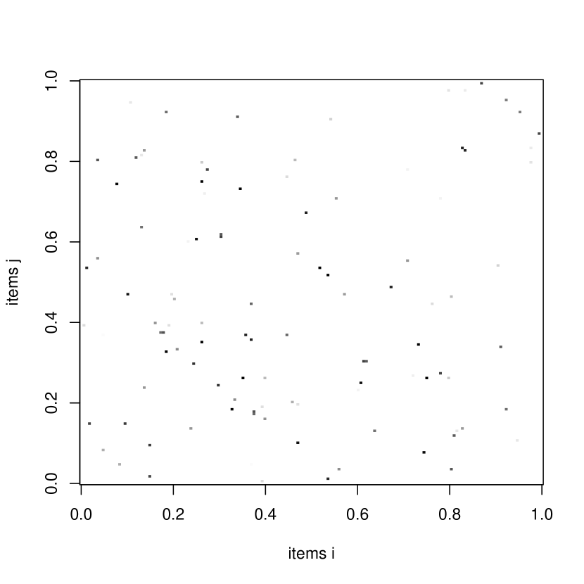
(a) simulated

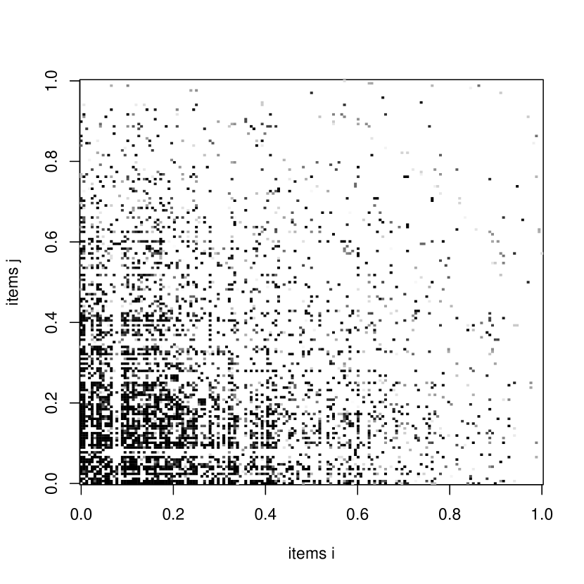
(b) Grocery

Figure 6: Hyper-confidence for rules with two items and $\gamma>0.99$ (items are ordered by decreasing support from left to right and bottom to top).

(a) simulated

(b) Grocery

Figure 7: Number of accepted rules depending on the used hyper-confidence threshold.

(c) simulated

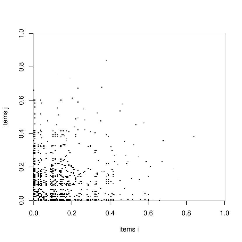
(d) Grocery

Figure 8: Hyper-confidence for rules with two items using a Bonferroni corrected $\gamma$.

Between the measures hyper-confidence and hyper-lift exists a direct connection. Using a threshold $\gamma$ on hyper-confidence and requiring a hyper-lift using the $\delta$ quantile to be greater than one is equivalent for $\gamma=\delta$. Formally, for an arbitrary rule $X\Rightarrow Y$ and $0<\gamma<1$,

$$\mathrm{hyper\mbox{-}confidence}(X\Rightarrow Y)\geq\gamma\Leftrightarrow\mathrm{hyper\mbox{-}lift}_{\delta}(X\Rightarrow Y)>1\quad\text{for}\quad\gamma=\delta.$$ (17)

To prove this equivalence, let us write $F(c)=P(C_{XY}\leq c)$ for the distribution function of $C_{XY}$, so that the hyper-confidence $h=h(c)$ equals $F(c-1)$. We note that $F$ as well as its quantile function $Q$ are non-decreasing and that for integer $c$ in the support of $C_{XY}$, $Q_{F(c)}=c$. Hence, provided that $h(c)>0$, $Q_{h(c)}=c-1$. What we need to show is that $h(c)\geq\gamma$ iff $c>Q_{\gamma}$. If $0<\gamma\leq h(c)$, it follows that $Q_{\gamma}\leq Q_{h(c)}=c-1$, i.e., $c>Q_{\gamma}$. Conversely, if $c>Q_{\gamma}$, it follows that $c-1\geq Q_{\gamma}$ and thus $h(c)=F(c-1)\geq F(Q_{\gamma})\geq\gamma$, completing the proof.

Hyper-confidence as defined above only uncovers complementary effects between items. To interpret using a threshold on hyper-confidence as a simple one-sided statistical test makes it also very natural to adapt the measure to find substitution effects, items which co-occur significantly less together than expected under independence. The hyper-confidence for substitutes is given by:

$$\mathrm{hyper\mbox{-}confidence}^{\mathrm{sub}}(X\Rightarrow Y)=P(C_{XY}>c_{XY})=1-\sum_{i=0}^{c_{XY}}P(C_{XY}=i)$$ (18)

Applying a threshold $\gamma^{\mathrm{sub}}$ can be again interpreted as using a one-sided test, this time for negatively related items. One could also construct a hyper-lift measure for substitutes using low quantiles; however, its construction is less straightforward.

In Figures 9(a) and (b) we show the rules with two items which surpass a $\gamma^{\mathrm{sub}}$ of 0.99 in the simulated and the Grocery database. In the simulated data we see that the 68 falsely found rules are regularly scattered over the lower left triangle. In the Grocery database, the 116 rules which contain substitutes are concentrated for a few items (the line clearly visible in Figure 9(b) corresponds to the item ‘canned beer’ which has a strong substitution effect for most other items). As for complements, it is possible to use Bonferroni correction.

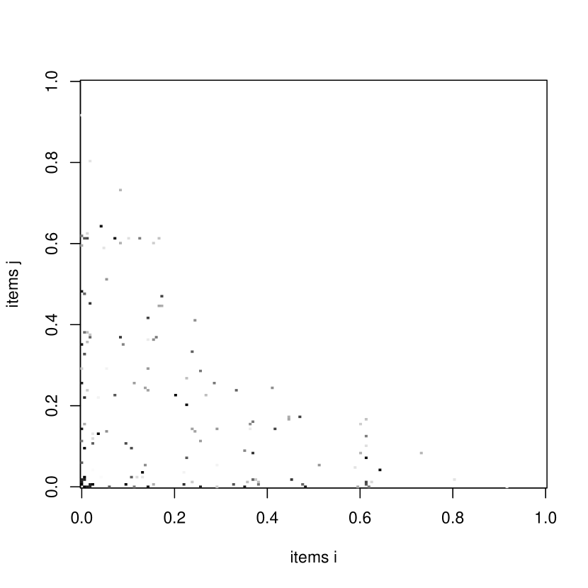
(a) simulated

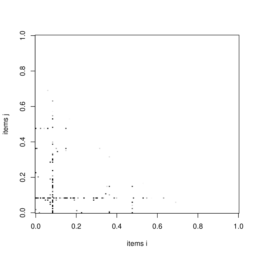
(b) Grocery

Figure 9: Hyper-confidence for substitutes with $\gamma^{\mathrm{sub}}>0.99$ for rules with two items.

4.3 Empirical results

To evaluate the proposed measures, we compare their ability to suppress spurious rules with the well-known lift measure. For the evaluation, we use in addition to the Grocery database two publicly available databases. The database “T10I4D100K” is an artificial data set generated by the procedure described by Agrawal and Srikant [4] which is often used to evaluate association rule mining algorithms. The third database is a sample of 50,000 transactions from the “Kosarak” database. This database was provided by Bodon [8] and contains click-stream data of a Hungarian on-line news portal. As shown in Table 3, the three databases have very different characteristics and thus should cover a wide range of applications for data from different sources and with different database sizes and numbers of items.

Database	Grocery	T10I4D100K	Kosarak
Type	market basket	artificial	click-stream
Transactions	9835	100,000	50,000
Avg. trans. size	4.41	10.10	3.00
Median trans. size	3.00	10.00	7.98
Distinct items	169	870	18,936

Table 3: Characteristics of the used databases.

For each database we simulate a comparable association-free data set following the simple probabilistic model described above in this paper. We generate all rules with one item in the right hand side which satisfy a specified minimum support (see Table 4). Then we compare the impact of lift and confidence with hyper-lift and hyper-confidence on rule selection. In Table 4 we present the number of rules found using the preset minimum support and the number of rules which also have a lift greater than $1$ and $2$, a hyper-lift with $\delta=0.99$ greater than $1$ and $2$, or a hyper-confidence greater than $0.9$ and $0.999$, respectively. From the results in the table we see that, compared to the real databases, in the simulated data sets only a much smaller number of rules reaches the required minimum support. This supports the assumption that these data sets do not contain associations between items while the real databases do. If we assume that rules found in the real databases are (at least potentially) useful associations while we know that rules found in the simulated data sets must be spurious, we can compare the performance of lift, hyper-lift and hyper-confidence on the data. In Table 4 we see that there obviously exists a trade-off between accepting more rules in the real databases while suppressing the spurious rules in the simulated data sets. In terms of rules found in the real databases versus rules suppressed in the simulated data sets, $\mathrm{hyper\mbox{-}lift_{0.99}}>1$ lies for all three databases between $\mathrm{lift}>1$ and $\mathrm{lift}>2$ while $\mathrm{hyper\mbox{-}lift_{0.99}}>2$ never accepts spurious rules but also reduces the rules in the real databases (especially in the Grocery database). The same is true for hyper-confidence with a threshold of $0.9$ the number of resulting rules lying in between the results for the two lift thresholds and for $0.999$ hyper-confidence only once (for the Grocery database) accepts a single rule.

Database	Grocery/	sim.	T10I4D100K/	sim.	Kosarak/	sim.
Min. support	0.001		0.001		0.002
Found rules	40943/	8685	89605/	9288	53245/	2530
$\mathrm{lift>1}$	40011/	5812	86855/	5592	51822/	1365
$\mathrm{lift>2}$	27334/	180	84880/	0	42641/	0
$\mathrm{hyper\mbox{-}lift}_{0.99}>1$	30083/	196	86463/	150	51151/	23
$\mathrm{hyper\mbox{-}lift}_{0.99}>2$	1563/	0	83176/	0	37683/	0
$\mathrm{hyper\mbox{-}conf.}>0.9$	36724/	1531	86647/	1286	51282/	240
$\mathrm{hyper\mbox{-}conf.}>0.9999$	15046/	1	86207/	0	51083/	0

Table 4: Number of rules exceeding a lift and hyper-lift ($\delta=0.99$) of 1 and 2, and a hyper-confidence of 0.9 and 0.9999 on the three databases and comparable simulated data sets.

(a) Grocery

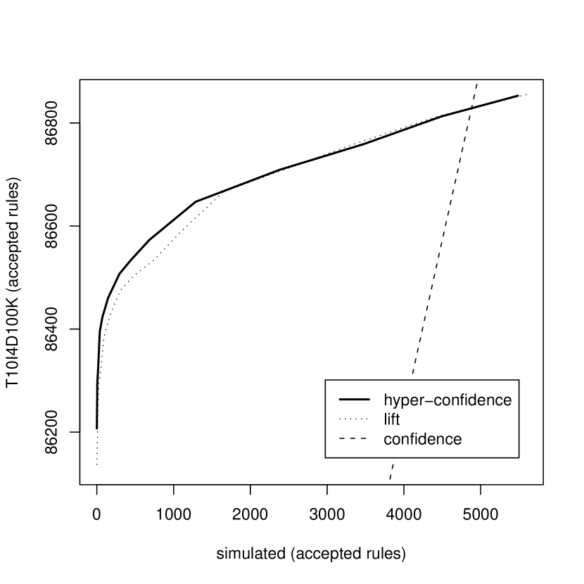
(b) T10I4D100K

(c) Kosarak

Figure 10: Comparison of number of rules accepted by different thresholds for lift, confidence, hyper-lift (only in the detail plots to the right) and hyper-confidence in the three databases and the simulated data sets.

To analyze the trade-off in more detail, we proceed as follows: We vary the threshold for lift (a minimum lift between 1 and 3) and assess the number of rules accepted in the databases and the simulated data sets for each setting. Then we repeat the procedure with confidence (a minimum between 0 and 1), with hyper-lift (a minimum hyper-lift between 1 and 3) at four settings for $\delta$ (0.9, 0.99, 0.999, 0.9999) and with hyper-confidence (a minimum threshold between 0.5 and 0.9999). We plot the number of accepted rules in the real database by the number of accepted rules in the simulated data sets where the points for each measure (lift, hyper-confidence, and hyper-lift with the same value for $\delta$) are connected by a line to form a curve. The resulting plots in Figure 10 are similar in spirit to Receiver Operating Characteristic (ROC) plots used in machine learning [25] to compare classifiers and can be interpreted similarly. Curves closer to the top left corner of the plot represent better results, since they provide a better ratio of true positives (here potentially useful rules accepted in the real databases) and false positives (spurious rules accepted in the simulated data sets) regardless of class or cost distributions.

Confidence performs considerably worse than the other measures and is only plotted in the left hand side plots. For the Kosarak database, confidence performs so badly that its curve lies even outside the plotting area.

Over the whole range of parameter values presented in the left hand side plots in Figure 10, there is only little difference visible between lift and hyper-confidence visible. The four hyper-lift curves are very close to the hyper-confidence curve and are omitted from the plot for better visibility. A closer inspection of the range with few spurious rules accepted in the simulated data sets (right hand side plots in Figure 10) shows that in this part hyper-confidence and hyper-lift clearly provides better results than lift (the new measures dominate lift). The performance of hyper-confidence and hyper-lift are comparable. The results for the Kosarak database look different than for the other two databases. The reason for this is that the generation process of click-stream data is very different from market basket data. For click-stream data the user clicks through a collection of Web pages. On each page the hyperlink structure confines the user’s choices to a usually very small subset of all pages. These restrictions are not yet incorporated into the probabilistic framework. However, hyper-lift and hyper-confidence do not depend on the framework and thus will produce still consistent results.

Note that in the previous evaluation, we did not know how many accepted rules in the real databases were spurious. However, we can speculate that if the new measures suppress noise better for the simulated data, it also produces better results in the real database and the improvement over lift is actually greater than can be seen in Figure 10.

Only for synthetic data sets, where we can fully control the generation process, we know which rules are non-spurious. We modified the generator described by Agrawal and Srikant [4] to report all itemsets which were used in generating the data set. These itemsets represent all non-spurious patterns contained in the data set. The default parameters for the generator to produce the data set T10I4D100K tend to produce easy to detect patterns since with the used so-called corruption level of 0.5 the 2000 patterns appear in the data set only slightly corrupted. We used a much higher corruption level of 0.9 which does not change the basic characteristics reported in Table 3 above but makes it considerably harder to find the non-spurious patterns.

We generated 100 data sets with 1000 items and 100,000 transactions each, where we saved all patterns used for the generation. For each data set, we generate sets of rules which satisfy a minimum support of 0.001 and different thresholds for hyper-confidence, lift and confidence (we omit hyper-lift here since the results are very close to hyper-confidence). For each set of rules, we count how many accepted rules represent patterns which were used for generating the corresponding data set (covered positive examples, P) and how many rules are spurious (covered negative examples, N). To compare the performance of the different measures in a single plot, we average the values for $P$ and $N$ for each measure at each used threshold and plot the results (Figure 11).

A plot of corresponding $P$ and $N$ values with all points for the same measure connected by a line is called a PN graph in the coverage space which is similar to the ROC space without normalizing the X and Y-axes [13]. PN graphs can be interpreted similarly to ROC graphs: Points closer to the top left corner indicate better performance. Coverage space is used in this evaluation since, other than most classifiers, association rules typically only cover a small fraction of all examples (only rules generated from frequent itemsets generate rules) which makes coverage space a more natural representation than ROC space.

Averaged PN graphs for hyper-confidence, lift, confidence and the $\chi^{2}$ statistic are presented in Figure 11. Hyper-confidence dominates lift by a considerably larger margin than in the previous experiments reported in Figure 10(b) above. This supports the speculation that the improvements achievable with hyper-confidence are also considerable for real world databases. Using a varying threshold on the $\chi^{2}$ statistic as proposed by Liu et al. [23] performs better than lift and provides only slightly inferior results than hyper-confidence.

We also inspected the results for the individual data sets. While the characteristics of the data sets vary sometimes significantly (due to the way the patterns used in the generation process are produced;  see [4]), all data sets show similar results with hyper-confidence dominating all other measures.

Figure 11: Average PN graph for 100 data sets generated with a corruption rate of 0.9.

5 Conclusion

In this contribution we used a simple independence model (a null model with “no structure”) to simulate a data set with comparable characteristics as a real-world data set from a grocery outlet. We visually compared the values of different measures of interestingness for all possible rules with two items. In the comparison we found the same problems for confidence and lift, which other authors already pointed out. However, these authors only argued with specially constructed and isolated example rules. The analysis used in this paper gives a better picture of how strongly these problems influence the process of selecting whole sets of rules. Confidence favors rules with high-support items in the right hand side of the rule. For databases with items with strongly varying support counts, this effect dominates confidence which makes it a bad measure for selecting or ranking rules. Lift has a strong tendency to produce the highest values for rules which just pass the set minimum support threshold. Selecting or ranking rules by lift will lead to very unstable results, since even small changes of the minimum support threshold will lead to very different rules being ranked highest.

Motivated by these problems, two novel measures of interestingness, hyper-lift and hyper-confidence, are developed. Both measures quantify the deviation of the data from a null model which models the co-occurrence count of two independent itemsets in a database. Hyper-lift is similar to lift but uses instead of the expected value a quantile from the corresponding hyper-geometric distribution. The distribution can be very skewed and thus hyper-lift can result in significantly different ordering of rules than lift. Hyper-confidence is defined as the probability of realizing a count smaller than the observed count and from its setup related to a one-sided Fisher’s exact test.

The new measures do not show the problematic behavior described for confidence and lift above. Also, both measures outperform confidence, lift, and the $\chi^{2}$ statistic on real-word data sets from different application domains as well as in an experiment with simulated data. This indicates that the knowledge of how independent itemsets co-occur can be used to construct superior measures of interestingness which improve the quality of the rule set returned by the mining algorithm.

A topic for future research is to develop more complicated independence models which incorporate constraints for specific application domains. For example, in click-stream data, the link structure restricts which pages can be reached from one page. Also the generation of artificial data sets which incorporate models for dependencies between items is an important area of research. Such data sets could greatly improve the way the effectiveness of data mining applications is evaluated and compared.

References

- Adamo [2001] J.-M. Adamo, Data Mining for Association Rules and Sequential Patterns, Springer, New York, 2001.
- Aggarwal and Yu [1998] C. C. Aggarwal and P. S. Yu, A new framework for itemset generation, in: PODS 98, Symposium on Principles of Database Systems, Seattle, WA, USA, 1998, pp. 18–24.
- Agrawal et al. [1993] R. Agrawal, T. Imielinski and A. Swami, Mining association rules between sets of items in large databases, in: Proceedings of the ACM SIGMOD International Conference on Management of Data, Washington D.C., 1993, pp. 207–216.
- Agrawal and Srikant [1994] R. Agrawal and R. Srikant, Fast algorithms for mining association rules in large databases, in: Proceedings of the 20th International Conference on Very Large Data Bases, VLDB, J. B. Bocca, M. Jarke and C. Zaniolo, eds., Santiago, Chile, 1994, pp. 487–499.
- Bayardo Jr. and Agrawal [1999] R. J. Bayardo Jr. and R. Agrawal, Mining the most interesting rules, in: Proceedings of the fifth ACM SIGKDD international conference on Knowledge discovery and data mining (KDD-99), ACM Press, 1999, pp. 145–154.
- Betancourt and Gautschi [1990] R. Betancourt and D. Gautschi, Demand complementarities, household production and retail assortments, Marketing Science 9 (1990), 146–161.
- Bock [1996] H. H. Bock, Probabilistic models in cluster analysis, Computational Statistics and Data Analysis 23 (1996), 5–29.
- Bodon [2003] F. Bodon, A fast apriori implementation, in: Proceedings of the IEEE ICDM Workshop on Frequent Itemset Mining Implementations (FIMI’03), B. Goethals and M. J. Zaki, eds., Melbourne, Florida, USA, 2003, volume 90 of CEUR Workshop Proceedings.
- Brin et al. [1997] S. Brin, R. Motwani, J. D. Ullman and S. Tsur, Dynamic itemset counting and implication rules for market basket data, in: SIGMOD 1997, Proceedings ACM SIGMOD International Conference on Management of Data, Tucson, Arizona, USA, 1997, pp. 255–264.
- Cadez et al. [2001] I. V. Cadez, P. Smyth and H. Mannila, Probabilistic modeling of transaction data with applications to profiling, visualization, and prediction, in: Proceedings of the ACM SIGKDD Intentional Conference on Knowledge Discovery in Databases and Data Mining (KDD-01), F. Provost and R. Srikant, eds., ACM Press, 2001, pp. 37–45.
- DuMouchel and Pregibon [2001] W. DuMouchel and D. Pregibon, Empirical Bayes screening for multi-item associations, in: Proceedings of the ACM SIGKDD Intentional Conference on Knowledge Discovery in Databases and Data Mining (KDD-01), F. Provost and R. Srikant, eds., ACM Press, 2001, pp. 67–76.
- Fisher [1935] R. A. Fisher, The Design of Experiments, Oliver and Boyd, Edinburgh, 1935.
- Fürnkranz and Flach [2005] J. Fürnkranz and P. A. Flach, Roc ’n’ rule learning – towards a better understanding of covering algorithms, Machine Learning 58 (2005), 39–77.
- Goethals and Zaki [2004] B. Goethals and M. J. Zaki, Advances in frequent itemset mining implementations: Report on FIMI’03, SIGKDD Explorations 6 (2004), 109–117.
- Hahsler [2006] M. Hahsler, A model-based frequency constraint for mining associations from transaction data, Data Mining and Knowledge Discovery 13 (2006), 137–166.
- Hahsler et al. [2006a] M. Hahsler, B. Grün and K. Hornik, arules: Mining Association Rules and Frequent Itemsets, 2006a, URL http://cran.r-project.org/, R package version 0.4-3.
- Hahsler et al. [2006b] M. Hahsler, K. Hornik and T. Reutterer, Implications of probabilistic data modeling for mining association rules, in: From Data and Information Analysis to Knowledge Engineering, Proceedings of the 29th Annual Conference of the Gesellschaft für Klassifikation e.V., University of Magdeburg, March 9–11, 2005, M. Spiliopoulou, R. Kruse, C. Borgelt, A. Nürnberger and W. Gaul, eds., Springer-Verlag, 2006b, Studies in Classification, Data Analysis, and Knowledge Organization, pp. 598–605.
- Hipp et al. [2000] J. Hipp, U. Güntzer and G. Nakhaeizadeh, Algorithms for association rule mining – A general survey and comparison, SIGKDD Explorations 2 (2000), 1–58.
- Hollmén et al. [2003] J. Hollmén, J. K. Seppänen and H. Mannila, Mixture models and frequent sets: Combining global and local methods for 0–1 data., in: SIAM International Conference on Data Mining (SDM’03), San Fransisco, 2003.
- Hruschka et al. [1999] H. Hruschka, M. Lukanowicz and C. Buchta, Cross-category sales promotion effects, Journal of Retailing and Consumer Services 6 (1999), 99–105.
- Johnson et al. [1993] N. L. Johnson, S. Kotz and A. W. Kemp, Univariate Discrete Distributions, John Wiley & Sons, New York, 2nd edition, 1993.
- Lehmann [1959] E. L. Lehmann, Testing Statistical Hypotheses, Wiley, New York, first edition, 1959.
- Liu et al. [1999] B. Liu, W. Hsu and Y. Ma, Mining association rules with multiple minimum supports, in: Proceedings of the fifth ACM SIGKDD international conference on Knowledge discovery and data mining (KDD-99), ACM Press, 1999, pp. 337–341.
- Pavlov et al. [2003] D. Pavlov, H. Mannila and P. Smyth, Beyond independence: Probabilistic models for query approximation on binary transaction data, IEEE Transactions on Knowledge and Data Engineering 15 (2003), 1409–1421.
- Provost and Fawcett [2001] F. Provost and T. Fawcett, Robust classification for imprecise environments, Machine Learning 42 (2001), 203–231.
- Shaffer [1995] J. P. Shaffer, Multiple hypothesis testing, Annual Review of Psychology 46 (1995), 561–584.
- Silverstein et al. [1998] C. Silverstein, S. Brin and R. Motwani, Beyond market baskets: Generalizing association rules to dependence rules, Data Mining and Knowledge Discovery 2 (1998), 39–68.
- Xiong et al. [2003] H. Xiong, P.-N. Tan and V. Kumar, Mining strong affinity association patterns in data sets with skewed support distribution, in: Proceedings of the IEEE International Conference on Data Mining, November 19–22, 2003, Melbourne, Florida, B. Goethals and M. J. Zaki, eds., 2003, pp. 387–394.