The Polychronakos–Frahm spin chain of $BC_{N}$ type and Berry–Tabor’s conjecture

Abstract

We compute the partition function of the su($m$) Polychronakos–Frahm spin chain of $BC_{N}$ type by means of the freezing trick. We use this partition function to study several statistical properties of the spectrum, which turn out to be analogous to those of other spin chains of Haldane–Shastry type. In particular, we find that when the number of particles is sufficiently large the level density follows a Gaussian distribution with great accuracy. We also show that the distribution of (normalized) spacings between consecutive levels is of neither Poisson nor Wigner type, but is qualitatively similar to that of the original Haldane–Shastry spin chain. This suggests that spin chains of Haldane–Shastry type are exceptional integrable models, since they do not satisfy a well-known conjecture of Berry and Tabor according to which the spacings distribution of a generic integrable system should be Poissonian. We derive a simple analytic expression for the cumulative spacings distribution of the $BC_{N}$-type Polychronakos–Frahm chain using only a few essential properties of its spectrum, like the Gaussian character of the level density and the fact the energy levels are equally spaced. This expression is in excellent agreement with the numerical data and, moreover, there is strong evidence that it can also be applied to the Haldane–Shastry and the Polychronakos–Frahm spin chains.

I Introduction

Solvable spin chains often provide a natural setting for testing or modeling interesting physical phenomena and mathematical results in such disparate fields as fractional statistics, random matrix theory or orthogonal polynomials. Among these chains, those of Haldane–Shastry (HS) type occupy a distinguished position due to their remarkable integrability and solvability properties. The original chain of this type was independently introduced twenty years ago by Haldane Haldane (1988) and Shastry Shastry (1988), in an attempt to construct a model whose ground state coincided with Gutzwiller’s variational wave function for the Hubbard model in the limit of large on-site interaction Hubbard (1963); Gutzwiller (1963); Gebhard and Vollhardt (1987). In the original HS chain, the spins are equally-spaced on a circle and present pairwise interactions inversely proportional to their chord distance.

An essential feature of the spin chains of HS type is their close connection with the spin versions of the Calogero Calogero (1971) and Sutherland Sutherland (1971, 1972) models, and their generalizations due to Olshanetsky and Perelomov Olshanetsky and Perelomov (1983). This observation —already pointed out by Shastry in his original paper— was elegantly formulated by Polychronakos in Ref. Polychronakos (1993). In the latter reference, the author showed that the original HS chain can be obtained from the spin Sutherland model Ha and Haldane (1992); Hikami and Wadati (1993); Minahan and Polychronakos (1993) in the strong coupling limit, in which the dynamical and spin degrees of freedom decouple, so that the particles “freeze” at the equilibrium positions of the scalar part of the potential. In this regime, the integrals of motion of the spin Sutherland model directly yield first integrals of the HS chain, thereby explaining its complete integrability. This procedure was also applied in Polychronakos (1993) to construct a new integrable spin chain related to the original Calogero model. The spectrum of this chain was numerically studied by Frahm Frahm (1993), who found that the levels are grouped in highly degenerate multiplets. In a subsequent publication, Polychronakos computed the partition function of this chain (usually referred to in the literature as the Polychronakos–Frahm chain) by the “freezing trick” argument described above Polychronakos (1994). Interestingly, the partition function of the original HS chain was computed only very recently Finkel and González-López (2005).

Both the HS and the PF (Polychronakos–Frahm) chains are obtained from the Sutherland and Calogero models associated with the $A_{N}$ root system in Olshanetsky and Perelomov’s approach. The $BC_{N}$ versions of both chains have also been studied in the literature. More precisely, the integrability of the PF chain of $BC_{N}$ type was established by Yamamoto and Tsuchiya Yamamoto and Tsuchiya (1996) using again the freezing trick. On the other hand, the partition function of the HS chain of $BC_{N}$ type was computed in closed form in Ref. Enciso et al. (2005). The explicit knowledge of the partition function made it possible to study certain statistical properties of the spectrum of this chain. In particular, it was observed that for a large number of spins the level density is Gaussian. As a matter of fact, this property also holds for the original HS chain, as shown in Ref. Finkel and González-López (2005). The analysis of the distribution of the spacing between consecutive levels of the original HS chain was also undertaken in the latter reference. Rather unexpectedly, it was found that this distribution is not of Poisson type, as should be the case for a “generic” integrable model according to a long-standing conjecture of Berry and Tabor Berry and Tabor (1977). This behavior has also been recently reported for a supersymmetric version of the HS chain Basu-Mallick and Bondyopadhaya (2006).

The aim of this paper is twofold. In the first place, we shall compute in closed form the partition function of the PF chain of $BC_{N}$ type by means of the freezing trick. Using the partition function, we shall perform a numerical study of the density of levels and the distribution of the spacing between consecutive energies. We shall see that the level density is again Gaussian, and that the spacings distribution is analogous to that of the original HS chain. In particular, our results show that the distribution of spacings is neither Poissonian nor of Wigner type (characteristic of chaotic systems). We shall next derive a simple analytic expression for the cumulative spacings distribution, which reproduces the numerical data with much greater accuracy than the empiric formula proposed in Ref. Finkel and González-López (2005). In fact, we have strong numerical evidence that the new expression can also be applied to the HS and PF chains of $A_{N}$ type. In view of the Berry–Tabor conjecture, our results suggest that spin chains of HS type are exceptional among the class of integrable models.

II The partition function of the PF chain of $BC_{N}$ type

The Hamiltonian of the (antiferromagnetic) su($m$) PF chain of $BC_{N}$ type is defined by

$${\mathcal{H}}^{\epsilon}=\sum_{i\neq j}\bigg{[}\frac{1+S_{ij}}{(\xi_{i}-\xi_{j})^{2}}+\frac{1+\tilde{S}_{ij}}{(\xi_{i}+\xi_{j})^{2}}\bigg{]}+\beta\sum_{i}\frac{1-\epsilon S_{i}}{\xi_{i}^{2}}\,,$$ (1)

where the sums run from $1$ to $N$ (as always hereafter, unless otherwise stated), $\beta>0$, $\epsilon=\pm 1$, $S_{ij}$ is the operator which permutes the $i$-th and $j$-th spins, $S_{i}$ is the operator reversing the $i$-th spin, and $\tilde{S}_{ij}=S_{i}S_{j}S_{ij}$. Note that the spin operators $S_{ij}$ and $S_{i}$ can be expressed in terms of the fundamental su($m$) spin generators $J^{\alpha}_{k}$ at the site $k$ (with the normalization $\operatorname{tr}(J^{\alpha}_{k}J^{\gamma}_{k})=\frac{1}{2}\delta^{\alpha\gamma}$) as

$$S_{ij}=\frac{1}{m}+2\sum_{\alpha=1}^{m^{2}-1}J_{i}^{\alpha}J_{j}^{\alpha}\,,\qquad S_{i}=\sqrt{2m}\,J^{1}_{i}\,.$$

The chain sites $\xi_{i}$ are the coordinates of the unique minimum in $C=\{\mathbf{x}\mid 0<x_{1}<\cdots<x_{N}\}$ of the potential

$$U(\mathbf{x})=\sum_{i\neq j}\bigg{[}\frac{1}{(x_{ij}^{-})^{2}}+\frac{1}{(x_{ij}^{+})^{2}}\bigg{]}+\sum_{i}\frac{\beta^{2}}{x_{i}^{2}}+\frac{r^{2}}{4}\,,$$ (2)

where $x_{ij}^{\pm}=x_{i}\pm x_{j}$ and $r^{2}=\sum_{i}x_{i}^{2}$. The existence of this minimum follows from the fact that $U$ tends to $+\infty$ on the boundary of $C$ and as $r\to\infty$, and its uniqueness was established in Ref. Corrigan and Sasaki (2002) by expressing the potential $U$ in terms of the logarithm of the ground state of the $BC_{N}$ Calogero model

$$H^{\mathrm{sc}}=-\sum_{i}\partial_{x_{i}}^{2}+a(a-1)\sum_{i\neq j}\bigg{[}\frac{1}{(x_{ij}^{-})^{2}}+\frac{1}{(x_{ij}^{+})^{2}}\bigg{]}\\ +b(b-1)\sum_{i}\frac{1}{x_{i}^{2}}+\frac{a^{2}}{4}\,r^{2}\,,$$ (3)

with $b=\beta a$ and $a>1/2$. Moreover, it can be shown Ahmed et al. (1979) that $\xi_{i}=\sqrt{2y_{i}}$, where $y_{i}$ is the $i$-th zero of the generalized Laguerre polynomial $L_{N}^{\beta-1}$. From this fact, one can infer Calogero and Perelomov (1978) that for $N\gg\beta$ the density of sites (normalized to unity) $\rho_{N}(x)$ is given by the circular law

$$\rho_{N}(x)=\frac{1}{2\pi N}\,\sqrt{8N-x^{2}}\,.$$ (4)

Note that in this limit the sites’ density is independent of $\beta$ and is qualitatively similar to that of the PF chain of $A_{N}$ type Frahm (1993). Integrating the previous equation, we obtain the implicit asymptotic relation

$$4\pi k=\xi_{k}\sqrt{8N-\xi_{k}^{2}}+8N\arcsin\Big{(}\frac{\xi_{k}}{\sqrt{8N}}\Big{)}\,,$$

valid also for $N\gg\beta$.

The spin chain (1) can be expressed in terms of the spin Calogero model of $BC_{N}$ type

$$H^{\epsilon}=-\sum_{i}\partial_{x_{i}}^{2}+a\sum_{i\neq j}\bigg{[}\frac{a+S_{ij}}{(x_{ij}^{-})^{2}}+\frac{a+\tilde{S}_{ij}}{(x_{ij}^{+})^{2}}\bigg{]}\\ +b\sum_{i}\frac{b-\epsilon S_{i}}{x_{i}^{2}}+\frac{a^{2}}{4}\,r^{2}$$ (5)

and its scalar reduction (3) as

$$H^{\epsilon}=H^{\mathrm{sc}}+a\,\widetilde{\mathcal{H}}^{\epsilon}\,,$$ (6)

where $\widetilde{\mathcal{H}}^{\epsilon}$ is obtained from ${\mathcal{H}}^{\epsilon}$ replacing the chain sites ${\boldsymbol{\xi}}$ by the particles’ coordinates $\mathbf{x}$. Since

$$H^{\epsilon}=-\sum_{i}\partial_{x_{i}}^{2}+a^{2}U+O(a)\,,$$

when the coupling constant $a$ tends to infinity the particles in the spin dynamical model (5) concentrate at the coordinates of the minimum of the potential $U$, that is at the sites $\xi_{i}$ of the chain (1). Thus, in the limit $a\to\infty$ the spin and dynamical degrees of freedom of the Hamiltonian (5) decouple, so that by Eq. (6) its eigenvalues are approximately given by

$$E^{\epsilon}_{ij}\simeq E^{\mathrm{sc}}_{i}+a{\mathcal{E}}^{\epsilon}_{j}\,,\qquad a\gg 1\,,$$ (7)

where $E^{\mathrm{sc}}_{i}$ and ${\mathcal{E}}^{\epsilon}_{j}$ are two arbitrary eigenvalues of $H^{\mathrm{sc}}_{i}$ and ${\mathcal{H}}^{\epsilon}$, respectively. The asymptotic relation (7) immediately yields the following exact formula for the partition function ${\mathcal{Z}}^{\epsilon}$ of the chain (1):

$${\mathcal{Z}}^{\epsilon}(T)=\lim_{a\to\infty}\frac{Z^{\epsilon}(aT)}{Z^{\mathrm{sc}}(aT)}\,,$$ (8)

where $Z^{\epsilon}$ and $Z^{\mathrm{sc}}$ are the partition functions of $H^{\epsilon}$ and $H^{\mathrm{sc}}$, respectively.

We shall next evaluate the partition function ${\mathcal{Z}}^{\epsilon}$ of the chain (1) by computing the partition functions $Z^{\epsilon}$ and $Z^{\mathrm{sc}}$ in Eq. (8). In order to determine the spectra of the corresponding Hamiltonians $H^{\epsilon}$ and $H^{\mathrm{sc}}$, following Ref. Finkel and González-López (2005) we introduce the auxiliary operator

$$H^{\prime}=-\sum_{i}\partial_{x_{i}}^{2} +\sum_{i\neq j}\bigg{[}\frac{a}{(x_{ij}^{-})^{2}}(a-K_{ij})+\frac{a}{(x_{ij}^{+})^{2}}(a-\widetilde{K}_{ij})\bigg{]}$$

$$+\sum_{i}\frac{b}{x_{i}^{2}}\,(b-K_{i})+\frac{a^{2}}{4}\,r^{2}\,,$$ (9)

where $K_{ij}$ and $K_{i}$ are coordinate permutation and sign reversing operators, defined by

$$(K_{ij}f)(x_{1},\dots,x_{i},\dots,x_{j},\dots,x_{N})$$

$$\hskip 85.00012pt=f(x_{1},\dots,x_{j},\dots,x_{i},\dots,x_{N})\,,$$

$$(K_{i}f)(x_{1},\dots,x_{i},\dots,x_{N})=f(x_{1},\dots,-x_{i},\dots,x_{N})\,,$$

and $\widetilde{K}_{ij}=K_{i}K_{j}K_{ij}$. We then have the obvious relations

$$H^{\epsilon}=H^{\prime}\big{|}_{K_{ij}\to-S_{ij},K_{i}\to\epsilon S_{i}}\,,$$ (10a)

$$H^{\mathrm{sc}}=H^{\prime}\big{|}_{K_{ij},K_{i}\to 1}\,.$$ (10b)

On the other hand, the spectrum of $H^{\prime}$ can be easily computed by noting that this operator can be written in terms of the rational Dunkl operators of $BC_{N}$ type Dunkl (1998)

$$J_{i}^{-}=\partial_{x_{i}} +a\sum_{j\neq i}\bigg{[}\frac{1}{x_{ij}^{-}}\,(1-K_{ij})+\frac{1}{x_{ij}^{+}}\,(1-\widetilde{K}_{ij})\bigg{]}$$

$$+\frac{b}{x_{i}}\,(1-K_{i})\,,\qquad i=1,\dots,N\,,$$ (11)

as follows Finkel et al. (2001):

$$H^{\prime}=\mu\Big{[}-\sum_{i}\big{(}J_{i}^{-}\big{)}^{2}+a\sum_{i}x_{i}\partial_{x_{i}}+E_{0}\Big{]}\mu^{-1}\,,$$ (12)

where

$$\mu(\mathbf{x})=\mathrm{e}^{-\frac{a}{4}\mspace{1.0mu}r^{2}}\prod_{i}|x_{i}|^{b}\cdot\prod_{i<j}{\big{|}x_{i}^{2}-x_{j}^{2}\big{|}}^{a}$$ (13)

is the ground state of the Hamiltonian (3) and

$$E_{0}=Na\Big{(}b+a(N-1)+\frac{1}{2}\Big{)}\,.$$ (14)

Since the Dunkl operators (11) map any monomial $\prod_{i}x_{i}^{n_{i}}$ into a polynomial of total degree $n_{1}+\cdots+n_{N}-1$, by Eq. (12) the operator $H^{\prime}$ is represented by an upper triangular matrix in the (non-orthonormal) basis with elements

$$\phi_{\mathbf{n}}=\mu\prod_{i}x_{i}^{n_{i}},\>\quad\mathbf{n}\equiv(n_{1},\dots,n_{N})\in{({\mathbb{N}}\cup\{0\})}^{N},$$ (15)

ordered according to the total degree $|\mathbf{n}|\equiv n_{1}+\cdots+n_{N}$ of the monomial part. More precisely,

$$H^{\prime}\phi_{\mathbf{n}}=E^{\prime}_{\mathbf{n}}\phi_{\mathbf{n}}+\sum_{|\bm{|}<|\mathbf{n}|}c_{\bm{\mathbf{n}}}\phi_{\bm{\,}},$$ (16)

where

$$E^{\prime}_{\mathbf{n}}=a\mspace{1.0mu}|\mathbf{n}|+E_{0}$$ (17)

and the coefficients $c_{\bm{\mathbf{n}}}$ are real constants.

We shall now construct a basis of the Hilbert space of the Hamiltonian $H^{\epsilon}$ in which this operator is also represented by an upper triangular matrix. To this end, let us denote by $\Lambda^{\epsilon}$ the projector on states antisymmetric under simultaneous permutations of spatial and spin coordinates, and with parity $\epsilon$ under sign reversals of coordinates and spins. If

$$|\mathbf{s}\rangle\equiv|s_{1},\dots,s_{N}\rangle,\quad s_{i}=-M,-M+1,\dots,M\equiv{\textstyle\frac{m-1}{2}},$$

denotes a state of the su($m$) spin basis, the functions

$$\psi_{\mathbf{n},\mathbf{s}}(\mathbf{x})=\Lambda^{\epsilon}\big{(}\phi_{\mathbf{n}}(\mathbf{x})|\mathbf{s}\rangle\big{)}\,,$$ (18)

form a basis of the Hilbert space of the Hamiltonian $H^{\epsilon}$ provided that:

(i)  $n_{1}\geqslant\cdots\geqslant n_{N}$.

(ii)  $s_{i}>s_{j}$ whenever $n_{i}=n_{j}$ and $i<j$.

(iii)  $s_{i}\geqslant 0$ for all $i$, and $s_{i}>0$ if $(-1)^{n_{i}}=-\epsilon$.

The first two conditions are a consequence of the antisymmetry of the states (18) under particle permutations, while the last condition is due to the fact that these states must have parity $\epsilon$ under sign reversals. Since $K_{ij}\Lambda^{\epsilon}=-S_{ij}\Lambda^{\epsilon}$ and $K_{i}\Lambda^{\epsilon}=\epsilon S_{i}\Lambda^{\epsilon}$, it follows that $H^{\epsilon}\Lambda^{\epsilon}=H^{\prime}\Lambda^{\epsilon}$. Using this identity and the fact that $H^{\prime}$ obviously commutes with $\Lambda^{\epsilon}$, from Eq. (16) we easily obtain

$$H^{\epsilon}\psi_{\mathbf{n},\mathbf{s}} =H^{\prime}\psi_{\mathbf{n},\mathbf{s}}=\Lambda^{\epsilon}\big{(}(H^{\prime}\phi_{\mathbf{n}})|\mathbf{s}\rangle\big{)}$$

$$=E^{\prime}_{\mathbf{n}}\psi_{\mathbf{n},\mathbf{s}}+\sum_{|\bm{|}<|\mathbf{n}|}c_{\bm{\mathbf{n}}}\psi_{\bm{,}\mathbf{s}}\,.$$

Thus $H^{\epsilon}$ is represented by an upper triangular matrix in the basis (18), ordered according to the degree $|\mathbf{n}|$. The diagonal elements of this matrix are given by

$$E^{\epsilon}_{\mathbf{n},\mathbf{s}}=a\mspace{1.0mu}|\mathbf{n}|+E_{0}\,,$$ (19)

where $\mathbf{n}$ and $\mathbf{s}$ satisfy conditions (i)–(iii) above. Note that, although the numerical value of $E^{\epsilon}_{\mathbf{n},\mathbf{s}}$ is independent of $\mathbf{s}$, the degeneracy of each level clearly depends on the spin through the latter conditions.

Turning next to the scalar Hamiltonian $H^{\mathrm{sc}}$, in view of Eq. (10b) we now need to consider scalar functions of the form

$$\psi_{\mathbf{n}}(\mathbf{x})=\Lambda_{s}\phi_{\mathbf{n}}(\mathbf{x})\,,$$ (20)

where $\Lambda_{s}$ is the symmetrizer with respect to both permutations and sign reversals. These functions form a (non-orthonormal) basis of the Hilbert space of $H^{\mathrm{sc}}$ provided that $n_{i}=2k_{i}$ are even integers and $k_{1}\geqslant\cdots\geqslant k_{N}$. Just as before, the matrix of the scalar Hamiltonian $H^{\mathrm{sc}}$ in the basis (20) ordered by the degree is upper triangular, with diagonal elements $E^{\mathrm{sc}}_{\mathbf{n}}$ also given by the RHS of (19).

Let us next compute the partition functions $Z^{\mathrm{sc}}$ and $Z^{\epsilon}$ of the models (3) and (5). To begin with, from now on we shall drop the common ground state energy $E_{0}$ in both models, since by Eq. (8) it does not contribute to the partition function ${\mathcal{Z}}^{\epsilon}$. With this convention, the partition function of the scalar Hamiltonian $H^{\mathrm{sc}}$ is given by

$$Z^{\mathrm{sc}}(aT)=\sum_{k_{1}\geqslant\cdots\geqslant k_{N}\geqslant 0}q^{2|\mathbf{k}|}\,,$$

where $q=\mathrm{e}^{-1/(k_{\mathrm{B}}T)}$. The previous sum can be evaluated by expressing it in terms of the differences $p_{i}=k_{i}-k_{i+1}$, $i=1,\dots,N-1$, with $p_{N}\equiv k_{N}$. Since $k_{j}=\sum\limits_{i=j}^{N}p_{i}$, we easily obtain

$$Z^{\mathrm{sc}}(aT) =\sum_{p_{1},\dots,p_{N}\geqslant 0}q^{2\sum\limits_{j=1}^{N}\sum\limits_{i=j}^{N}p_{i}}=\sum_{p_{1},\dots,p_{N}\geqslant 0}q^{2\sum\limits_{i=1}^{N}ip_{i}}$$

$$=\prod_{i}\sum_{p_{i}\geqslant 0}{(q^{2i})}^{p_{i}}=\prod_{i}(1-q^{2i})^{-1}\,.$$ (21)

In order to compute the partition function of the spin Hamiltonian $H^{\epsilon}$, we shall first assume that $m$ is even, so that condition (iii) simplifies to

(iii^′)   $s_{i}>0$ for all $i$.

As neither the value of $E^{\epsilon}_{\mathbf{n},\mathbf{s}}$ nor conditions (i), (ii) and (iii^′) depend on $\epsilon$, in this case the partition functions $Z^{\epsilon}$ and ${\mathcal{Z}}^{\epsilon}$ cannot depend on $\epsilon$. Hence from now on we shall drop the superscript $\epsilon$ when $m$ is even, writing simply $Z$ and ${\mathcal{Z}}$. By Eq. (19), after dropping $E_{0}$ the partition function of the Hamiltonian (5) can be written as

$$Z(aT)=\sum_{n_{1}\geqslant\cdots\geqslant n_{N}\geqslant 0}d_{\mathbf{n}}\mspace{1.0mu}q^{|\mathbf{n}|}\,,$$ (22)

where the spin degeneracy factor $d_{\mathbf{n}}$ is the number of spin states $|\mathbf{s}\rangle$ satisfying conditions (ii) and (iii^′). Writing

$$\mathbf{n}=\big{(}\overbrace{\vphantom{1}k_{1},\dots,k_{1}}^{\nu_{1}},\dots,\overbrace{\vphantom{1}k_{r},\dots,k_{r}}^{\nu_{r}}\big{)},\qquad k_{1}>\cdots>k_{r}\geqslant 0,$$

by conditions (ii) and (iii^′) we have

$$d_{\mathbf{n}}=\prod\limits_{i=1}^{r}\binom{m/2}{\nu_{i}}\equiv d({\boldsymbol{\nu}})\,,\qquad{\boldsymbol{\nu}}=(\nu_{1},\dots,\nu_{r})\,.$$ (23)

Note that $\sum_{i=1}^{r}\nu_{i}=N$, so that the multiindex ${\boldsymbol{\nu}}$ can be regarded as an element of the set ${\mathcal{P}}_{N}$ of partitions of $N$ (taking order into account). With the previous notation, Eq. (22) becomes

$$Z(aT) =\sum_{{\boldsymbol{\nu}}\in{\mathcal{P}}_{N}}d({\boldsymbol{\nu}})\sum_{k_{1}>\cdots>k_{r}\geqslant 0}\,q^{\sum\limits_{i=1}^{r}\nu_{i}k_{i}}$$

$$=\sum_{{\boldsymbol{\nu}}\in{\mathcal{P}}_{N}}d({\boldsymbol{\nu}})\sum_{\begin{subarray}{c}p_{1},\dots,p_{r-1}>0\\ p_{r}\geqslant 0\end{subarray}}q^{\sum\limits_{i=1}^{r}\nu_{i}\sum\limits_{j=i}^{r}p_{j}}$$

$$=\sum_{{\boldsymbol{\nu}}\in{\mathcal{P}}_{N}}d({\boldsymbol{\nu}})\sum_{\begin{subarray}{c}p_{1},\dots,p_{r-1}>0\\ p_{r}\geqslant 0\end{subarray}}\,\prod_{j=1}^{r}q^{p_{j}\sum\limits_{i=1}^{j}\nu_{i}}$$

$$=q^{-N}\sum_{{\boldsymbol{\nu}}\in{\mathcal{P}}_{N}}d({\boldsymbol{\nu}})\prod_{j=1}^{r}\frac{q^{N_{j}}}{1-q^{N_{j}}}\,,$$ (24)

where

$$N_{j}=\sum_{i=1}^{j}\nu_{i}\,.$$

From Eqs. (8), (21) and (24) we finally obtain the following explicit expression for the partition function of the $\mathrm{su}(m)$ PF chain of $BC_{N}$ type in the case of even $m$:

$${\mathcal{Z}}(T)=q^{-N}\prod_{i}(1-q^{2i})\sum_{{\boldsymbol{\nu}}\in{\mathcal{P}}_{N}}d({\boldsymbol{\nu}})\prod_{j=1}^{\ell({\boldsymbol{\nu}})}\frac{q^{N_{j}}}{1-q^{N_{j}}}\,,$$ (25)

where $\ell({\boldsymbol{\nu}})=r$ is the number of components of the multiindex ${\boldsymbol{\nu}}$. For instance, for spin $1/2$ we have $\nu_{i}=1$ for all $i$, and therefore $r=N$, $d({\boldsymbol{\nu}})=1$ and $N_{j}=j$, so that the previous formula simplifies to

$${\mathcal{Z}}(T)=q^{\frac{1}{2}N(N-1)}\prod_{i}(1+q^{i})\,,\qquad m=2\,.$$ (26)

Thus, for spin $1/2$ the spectrum of the chain (1) is given by

$${\mathcal{E}}_{j}=\frac{1}{2}\,N(N-1)+j\,,\qquad j=0,1,\dots,\frac{1}{2}\,N(N+1)\,,$$ (27)

and the degeneracy of the energy ${\mathcal{E}}_{j}$ is the number $Q_{N}(j)$ of partitions of the integer $j$ into distinct parts no larger than $N$ (with $Q_{N}(0)\equiv 1$). For $j\leqslant N$ this number coincides with the number $Q(j)$ of partitions of $j$ into distinct parts, which has been extensively studied in the mathematical literature Andrews (1976). It is also interesting to observe that the partition function (26) is closely related to Ramanujan’s fifth order mock theta function Hardy et al. (2000)

$$\psi_{1}(q)=\sum_{N=0}^{\infty}q^{N}{\mathcal{Z}}_{N}(q)\,,$$

where ${\mathcal{Z}}_{N}(q)$ denotes the RHS of Eq. (26).

Equation (26) shows that for spin $1/2$ the chain (1) is equivalent to a system of $N$ species of noninteracting fermions (with vacuum energy ${\mathcal{E}}_{0}=N(N-1)/2$), whose effective Hamiltonian is given by

$$H_{\text{eff}}={\mathcal{E}}_{0}+\sum_{i=1}^{N}E_{i}\,b^{\dagger}_{i}b_{i}\,.$$

Here $b_{i}$ (resp. $b^{\dagger}_{i}$) is the annihilation (resp. creation) operator of the $i$-th species of fermion, and $E_{i}=i$ its energy. A similar result was obtained in Ref. Basu-Mallick et al. (2008) for the supersymmetric $\mathrm{su}(1|1)$ (ferromagnetic) HS chain, although in the latter case the energy of the $i$-th fermion is $E_{i}=i(N-i)$ (the dispersion relation of the original Haldane–Shastry chain).

Let us consider now the case of odd $m$. In this case, it is convenient to slightly modify condition (i) above by first grouping the components of $\mathbf{n}$ with the same parity and then ordering separately the even and odd components. In other words, we shall write $\mathbf{n}=(\mathbf{n}_{\mathrm{e}},\mathbf{n}_{\mathrm{o}})$, where

$$\mathbf{n}_{\mathrm{e}}=\big{(}\overbrace{\vphantom{1}2k_{1},\dots,2k_{1}}^{\nu_{1}},\dots,\overbrace{\vphantom{1}2k_{s},\dots,2k_{s}}^{\nu_{s}}\big{)},$$

$$\mathbf{n}_{\mathrm{o}}=\big{(}\overbrace{\vphantom{1}2k_{s+1}+1,\dots,2k_{s+1}+1}^{\nu_{s+1}},\dots,\overbrace{\vphantom{1}2k_{r}+1,\dots,2k_{r}+1}^{\nu_{r}}\big{)},$$

and

$$k_{1}>\cdots>k_{s}\geqslant 0,\qquad k_{s+1}>\cdots>k_{r}\geqslant 0\,.$$

By conditions (ii) and (iii), the spin degeneracy factor is now

$$d_{\mathbf{n}}^{\epsilon}=\prod\limits_{i=1}^{s}\binom{\frac{m+\epsilon}{2}}{\nu_{i}}\cdot\prod\limits_{i=s+1}^{r}\binom{\frac{m-\epsilon}{2}}{\nu_{i}}\equiv d^{\epsilon}_{s}({\boldsymbol{\nu}})\,.$$ (28)

Calling

$$\tilde{N}_{j}=\sum_{i=s+1}^{j}\nu_{i}\,,\qquad j=s+1,\dots,r\,,$$

and proceeding as before, we obtain

$$Z^{\epsilon}(aT) =\sum_{{\boldsymbol{\nu}}\in{\mathcal{P}}_{N}}\sum_{s=0}^{r}d^{\epsilon}_{s}({\boldsymbol{\nu}})\sum_{\begin{subarray}{c}k_{1}>\cdots>k_{s}\geqslant 0\\ k_{s+1}>\cdots>k_{r}\geqslant 0\end{subarray}}q^{\sum\limits_{i=1}^{s}2\nu_{i}k_{i}}q^{\sum\limits_{i=s+1}^{r}\nu_{i}(2k_{i}+1)}$$

$$=\sum_{{\boldsymbol{\nu}}\in{\mathcal{P}}_{N}}\sum_{s=0}^{r}d^{\epsilon}_{s}({\boldsymbol{\nu}})\,q^{\tilde{N}_{r}}\Bigg{[}\sum_{k_{1}>\cdots>k_{s}\geqslant 0}q^{\sum\limits_{i=1}^{s}2\nu_{i}k_{i}}\Bigg{]}$$

$$\hskip 65.50012pt{}\times\Bigg{[}\sum_{k_{s+1}>\cdots>k_{r}\geqslant 0}q^{\sum\limits_{i=s+1}^{r}2\nu_{i}k_{i}}\Bigg{]}$$

$$=\sum_{{\boldsymbol{\nu}}\in{\mathcal{P}}_{N}}\sum_{s=0}^{\ell({\boldsymbol{\nu}})}d^{\epsilon}_{s}({\boldsymbol{\nu}})\,q^{-(N+N_{s})}\prod_{j=1}^{s}\frac{q^{2N_{j}}}{1-q^{2N_{j}}}$$

$$\hskip 65.50012pt{}\times\prod_{j=s+1}^{\ell({\boldsymbol{\nu}})}\frac{q^{2\tilde{N}_{j}}}{1-q^{2\tilde{N}_{j}}}\,.$$ (29)

Substituting the previous expression and (21) into (8), we immediately deduce the following explicit formula for the partition functions of the $\mathrm{su}(m)$ PF chain of $BC_{N}$ type for odd $m$:

$${\mathcal{Z}}^{\epsilon}(T)=\prod_{i}(1-q^{2i})\sum_{{\boldsymbol{\nu}}\in{\mathcal{P}}_{N}}\sum_{s=0}^{\ell({\boldsymbol{\nu}})}d^{\epsilon}_{s}({\boldsymbol{\nu}})\,q^{-(N+N_{s})}\\ {}\times\prod_{j=1}^{s}\frac{q^{2N_{j}}}{1-q^{2N_{j}}}\,\,\cdot\!\!\prod_{j=s+1}^{\ell({\boldsymbol{\nu}})}\frac{q^{2\tilde{N}_{j}}}{1-q^{2\tilde{N}_{j}}}\,.$$ (30)

Although we have chosen, for definiteness, to study the antiferromagnetic chain (1), a similar analysis can be performed for its ferromagnetic counterpart

$${\mathcal{H}}^{\epsilon}_{\mathrm{F}}=\sum_{i\neq j}\bigg{[}\frac{1-S_{ij}}{(\xi_{i}-\xi_{j})^{2}}+\frac{1-\tilde{S}_{ij}}{(\xi_{i}+\xi_{j})^{2}}\bigg{]}+\beta\sum_{i}\frac{1-\epsilon S_{i}}{\xi_{i}^{2}}\,.$$ (31)

Since now

$$H^{\epsilon}_{\mathrm{F}}=H^{\prime}\big{|}_{K_{ij}\to S_{ij},K_{i}\to\epsilon S_{i}}\,,$$ (32)

we must replace the operator $\Lambda^{\epsilon}$ in Eq. (18) by the projector on states symmetric under simultaneous permutations of the particles’ spatial and spin coordinates, and with parity $\epsilon$ under sign reversal of coordinates and spin. Hence condition (ii) above on the basis states $\psi_{\mathbf{n},\mathbf{s}}$ should now read

(ii^′) $s_{i}\geqslant s_{j}$ whenever $n_{i}=n_{j}$ and $i<j$.

As a result, the degeneracy factors $d({\boldsymbol{\nu}})$ and $d^{\epsilon}({\boldsymbol{\nu}})$ in Eqs. (23) and (28) should be replaced by their “bosonic” versions

$$d_{\mathrm{F}}({\boldsymbol{\nu}}) =\prod\limits_{i=1}^{r}\binom{\frac{m}{2}+\nu_{i}-1}{\nu_{i}}\,,$$

$$d_{\mathrm{F}}^{\epsilon}({\boldsymbol{\nu}}) =\prod\limits_{i=1}^{s}\binom{\frac{m+\epsilon}{2}+\nu_{i}-1}{\nu_{i}}\cdot\prod\limits_{i=s+1}^{r}\binom{\frac{m-\epsilon}{2}+\nu_{i}-1}{\nu_{i}}\,.$$

Therefore the partition function of the ferromagnetic $\mathrm{su}(m)$ PF chain of $BC_{N}$ type (31) is still given by Eq. (25) (for even $m$) or (30) (for odd $m$), but with $d({\boldsymbol{\nu}})$ and $d^{\epsilon}({\boldsymbol{\nu}})$ replaced respectively by $d_{\mathrm{F}}({\boldsymbol{\nu}})$ and $d^{\epsilon}_{\mathrm{F}}({\boldsymbol{\nu}})$.

On the other hand, the chains (1) and (31) are obviously related by

$${\mathcal{H}}^{\epsilon}_{\mathrm{F}}+{\mathcal{H}}^{-\epsilon}=2\Big{(}\sum_{i\neq j}\big{[}(\xi_{i}-\xi_{j})^{-2}+(\xi_{i}+\xi_{j})^{-2}\big{]}+\beta\sum_{i}\xi_{i}^{-2}\Big{)}\,.$$

The RHS of this equation clearly coincides with the largest eigenvalue ${\mathcal{E}}_{\mathrm{max}}$ of the antiferromagnetic chains ${\mathcal{H}}^{\epsilon}$, whose corresponding eigenvectors are the spin states symmetric under permutations and with parity $\epsilon$ under spin reversal. This eigenvalue is most easily computed for the spin $1/2$ chains, since in this case the spectrum is explicitly given in Eq. (27). We thus obtain

$${\mathcal{E}}_{\mathrm{max}}=\frac{1}{2}\,N(N-1)+\frac{1}{2}\,N(N+1)=N^{2}\,,$$ (33)

so that

$${\mathcal{H}}^{\epsilon}_{\mathrm{F}}=N^{2}-{\mathcal{H}}^{-\epsilon}\,.$$

Hence the partition functions ${\mathcal{Z}}^{\epsilon}$ and ${\mathcal{Z}}_{\mathrm{F}}^{\epsilon}$ of ${\mathcal{H}}^{\epsilon}$ and ${\mathcal{H}}^{\epsilon}_{\mathrm{F}}$ satisfy the remarkable identity

$${\mathcal{Z}}_{\mathrm{F}}^{\epsilon}(q)=q^{N^{2}}{\mathcal{Z}}^{-\epsilon}(q^{-1})\,.$$

This is a manifestation of the boson-fermion duality discussed in detail in Ref. Basu-Mallick et al. (2007) for the $\mathrm{su}(m|n)$ supersymmetric HS spin chain, since the ferromagnetic (resp. antiferromagnetic) chain can be regarded as purely bosonic (resp. fermionic). For instance, using the latter identity and Eq. (26) we easily obtain the following expression for the partition function of the ferromagnetic spin $1/2$ chains:

$${\mathcal{Z}}_{\mathrm{F}}(T)=\prod_{i}(1+q^{i})\,,\qquad m=2\,.$$ (34)

(Note that, as in the antiferromagnetic case, ${\mathcal{Z}}^{\epsilon}_{\mathrm{F}}$ is actually independent of $\epsilon$ for even $m$.) This is, again, the partition function of a system of $N$ species of free fermions of energy $E_{i}=i$, but now the vacuum energy vanishes.

Equation (25) for the partition function of the antiferromagnetic chains with even $m$ can be easily simplified to

$${\mathcal{Z}}(T)=\prod_{i}(1+q^{i})\sum_{{\boldsymbol{\nu}}\in{\mathcal{P}}_{N}}d({\boldsymbol{\nu}})\,q^{\sum\limits_{j=1}^{\ell({\boldsymbol{\nu}})-1}\kern-5.0ptN_{j}}\,\prod_{j=1}^{N-\ell({\boldsymbol{\nu}})}(1-q^{N_{j}^{\prime}})\,,$$

where the positive integers $N^{\prime}_{j}$ are defined by

$$\big{\{}N_{1}^{\prime},\dots,N^{\prime}_{N-\ell({\boldsymbol{\nu}})}\big{\}}=\big{\{}1,\dots,N-1\big{\}}-\big{\{}N_{1},\dots,N_{\ell({\boldsymbol{\nu}})-1}\big{\}}.$$

The sum in the RHS is easily recognized as the partition function ${\mathcal{Z}}^{(A)}(T;m/2)$ of the $\mathrm{su}(m/2)$ (antiferromagnetic) PF chain of $A_{N}$ type Basu-Mallick and Bondyopadhaya (2006). We thus obtain the remarkable factorization

$${\mathcal{Z}}(T;m)={\mathcal{Z}}_{\mathrm{F}}(T;2)\cdot{\mathcal{Z}}^{(A)}(T;m/2)\,,\quad m\in 2{\mathbb{N}}\,,$$ (35)

where the second argument in ${\mathcal{Z}}$ and ${\mathcal{Z}}_{\mathrm{F}}$ denotes the number of internal degrees of freedom. Replacing $d({\boldsymbol{\nu}})$ by $d_{\mathrm{F}}({\boldsymbol{\nu}})$ in Eq. (25) we obtain a similar factorization for the partition function of the ferromagnetic chains:

$${\mathcal{Z}}_{\mathrm{F}}(T;m)={\mathcal{Z}}_{\mathrm{F}}(T;2)\cdot{\mathcal{Z}}^{(A)}_{\mathrm{F}}(T;m/2)\,,\quad m\in 2{\mathbb{N}}\,.$$ (36)

Thus, for even $m$ the PF chains of $BC_{N}$ type (1) and (31) can be described by an effective model of two simpler noninteracting chains. This remarkable property, which to the best of our knowledge is unique among the class of chains of Haldane–Shastry type, certainly deserves further investigation.

III Spacings distribution and the Berry–Tabor conjecture

For fixed values of the number of particles $N$ and the internal degrees of freedom $m$, it is straightforward to obtain the spectrum of the chain (1) by expanding in powers of $q$ the expressions (25) or (30) for its partition function. In this way, we have been able to compute the spectrum of the latter chain for relatively large values of $N$ (for instance, up to $N=22$ for $m=3$). Our calculations conclusively show that the spectrum consists of a set of consecutive integers. For even $m$, this observation follows immediately from the expression (34)-(35) and the fact the the energies of the PF chain of $A_{N}$ type are also consecutive integers. For odd $m$ we have been unable to deduce this property from Eq. (30) for the partition function, although we have verified it numerically for many different values of $N$ and $m$.

Our computations also evidence that for $N\gtrsim 10$ the level density (normalized to unity) can be approximated with great accuracy by a normal distribution

$$g({\mathcal{E}})=\frac{1}{\sqrt{2\pi}\sigma}\,\mathrm{e}^{-\frac{({\mathcal{E}}-\mu)^{2}}{2\sigma^{2}}}\,,$$ (37)

where $\mu$ and $\sigma$ are respectively the mean and the variance of the energy. For instance, in Fig. 1 we compare the cumulative level density

$$F({\mathcal{E}})=m^{-N}\sum_{i;{\mathcal{E}}_{i}\leqslant{\mathcal{E}}}d_{i}\,,$$

where ${\mathcal{E}}_{i}$ is the $i$-th energy and $d_{i}$ its degeneracy, with the cumulative Gaussian density

$$G({\mathcal{E}})=\int_{-\infty}^{{\mathcal{E}}}g({\mathcal{E}}^{\prime})\,\mathrm{d}{\mathcal{E}}^{\prime}=\frac{1}{2}\bigg{[}1+\operatorname{erf}\bigg{(}\frac{{\mathcal{E}}-\mu}{\sqrt{2}\,\sigma}\bigg{)}\bigg{]}$$ (38)

for $N=15$ and $m=2$.

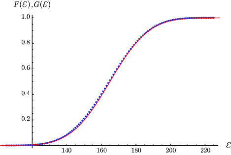
Figure 1: Cumulative distribution functions $F({\mathcal{E}})$ (at its discontinuity points) and $G({\mathcal{E}})$ (continuous red line) for $N=15$ and spin $1/2$.

Note, in this respect, that the approximately Gaussian character of the level density has already been verified for other chains of HS type, like the original Haldane–Shastry chain Finkel and González-López (2005), its $\mathrm{su}(m|n)$ supersymmetric version Basu-Mallick and Bondyopadhaya (2006), and the HS spin chain of $BC_{N}$ type Enciso et al. (2005).

The mean energy $\mu$ and its standard deviation $\sigma^{2}$, which by the previous discussion characterize the approximate level density of the chain (1) for large $N$, can be computed in closed form. Indeed, in Appendix A we show that

$$\mu =\frac{1}{2}\,\Big{(}1+\frac{1}{m}\Big{)}N^{2}-\frac{N}{2m}\,(1+\epsilon\mspace{1.0mu}p),$$ (39)

$$\sigma^{2} =\frac{N}{36}\,(4N^{2}+6N-1)\Big{(}1-\frac{1}{m^{2}}\Big{)}+\frac{N(1-p)}{4m^{2}}\,,$$ (40)

where $p\in\{0,1\}$ is the parity of $m$. Thus, when $N$ tends to infinity $\mu$ and $\sigma^{2}$ respectively diverge as $N^{2}$ and $N^{3}$, as for the original Polychronakos–Frahm chain . By contrast, it is known that $\mu\sim N^{3}$ and $\sigma^{2}\sim N^{5}$ for the trigonometric HS chains of both $A_{N}$ Finkel and González-López (2005) and $BC_{N}$ Enciso et al. (2005) types. It is also interesting to observe that the standard deviation of the energy is independent of $\epsilon$ even for odd $m$, when the spectrum does depend on $\epsilon$ according to the previous section’s results on the partition function.

We have next studied the probability density $p(s)$ of the spacing $s$ between consecutive (unfolded) levels of the chain (1). For many important integrable systems it is known that $p(s)$ is Poissonian Poilblanc et al. (1993); d’Auriac et al. (2002), in agreement with a well-known conjecture of Berry and Tabor Berry and Tabor (1977). On the other hand, it has been recently shown that for the HS chain of $A_{N}$ type Finkel and González-López (2005) (and its supersymmetric extension Basu-Mallick and Bondyopadhaya (2006)) the cumulative density $P(s)=\int_{0}^{s}p(x)\mathrm{d}x$ is well approximated by an empiric law of the form

$$\widetilde{P}(s)=\bigg{(}\frac{s}{s_{\mathrm{max}}}\bigg{)}^{\alpha}\Bigg{[}1-\gamma\bigg{(}1-\frac{s}{s_{\mathrm{max}}}\bigg{)}^{\beta}\Bigg{]}\,,$$ (41)

where $s_{\mathrm{max}}$ is the largest normalized spacing and $\alpha,\beta$ are adjustable parameters in the interval $(0,1)$. The parameter $\gamma$ is fixed by requiring that the average spacing be equal to $1$, with the result

$$\gamma=\Big{(}\frac{1}{s_{\mathrm{max}}}-\frac{\alpha}{\alpha+1}\Big{)}\Big{/}B(\alpha+1,\beta+1)\,,$$ (42)

where $B$ is Euler’s Beta function. Thus, the cumulative density of spacings for the HS chains of $A_{N}$ type follows neither Poisson’s nor Wigner’s law

$$P(s)=1-\mathrm{e}^{-\pi s^{2}/4},$$

characteristic of a chaotic system. Our aim is to ascertain whether the cumulative density of spacings for the PF chain of $BC_{N}$ type (1) resembles that of the $A_{N}$-type HS chain, or is rather Poissonian as expected for a generic integrable model.

In order to compare the spacings distributions of spectra with different level densities, it is necessary to transform the “raw” spectrum by applying what is known as the unfolding mapping Haake (2001). This mapping is defined by decomposing the cumulative level density $F({\mathcal{E}})$ as the sum of a fluctuating part $F_{\mathrm{f{}l}}({\mathcal{E}})$ and a continuous part $\eta({\mathcal{E}})$, which is then used to transform each energy ${\mathcal{E}}_{i}$, $i=1,\dots,n$, into an unfolded energy $\eta_{i}=\eta({\mathcal{E}}_{i})$. In this way one obtains a uniformly distributed spectrum $\{\eta_{i}\}_{i=1}^{n}$, regardless of the initial level density. One finally considers the normalized spacings $s_{i}=(\eta_{i+1}-\eta_{i})/\Delta$, where $\Delta=(\eta_{n}-\eta_{1})/(n-1)$ is the mean spacing of the unfolded energies, so that $\{s_{i}\}_{i=1}^{n-1}$ has unit mean.

By the above discussion, in our case we can take the unfolding mapping $\eta({\mathcal{E}})$ as the cumulative Gaussian distribution (38), with parameters $\mu$ and $\sigma$ respectively given by (39) and (40). Just as for the level density, in order to compare the discrete distribution function $p(s)$ with a continuous distribution it is more convenient to work with the cumulative spacings distribution $P(s)$. Our computations show that for a wide range of values of $N$, $m$ and $\epsilon=\pm 1$, the distribution $P(s)$ is well approximated by the empiric law (41) with suitable values of $\alpha$ and $\beta$. For instance, for $N=20$ and $m=2$ the largest spacing is $s_{\mathrm{max}}=3.13$, and the least-squares fit parameters $\alpha$ and $\beta$ are respectively $0.29$ and $0.24$, with a mean square error of $6.0{{\times}}10^{-4}$ (see Fig. 2).

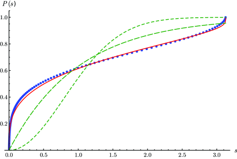
Figure 2: Cumulative spacings distribution $P(s)$ and its approximation $\widetilde{P}(s)$ (continuous red line) for $N=20$ and $m=2$. For convenience, we have also represented Poisson’s (green, long dashes) and Wigner’s (green, short dashes) cumulative distributions.

Thus the PF spin chain of $BC_{N}$ type behaves in this respect as the HS chain of $A_{N}$ type, and unlike most known integrable systems. In fact, we have also studied the spacings’ distribution of the original ($A_{N}$-type) PF chain, obtaining completely similar results [35]. These results (and also those of Ref. Basu-Mallick and Bondyopadhaya (2006)) suggest that a spacings distribution qualitatively similar to the empiric law (41) is characteristic of all spin chains of HS type.

Our next objective is to explain this characteristic behavior of the cumulative spacings distribution $P(s)$ of the chain (1) using only a few essential properties of its spectrum. We shall find a simple analytic expression without any adjustable parameters approximating $P(s)$ even better than the empiric law (41). Moreover, we have strong numerical evidence that the new expression also provides a very accurate approximation to the cumulative spacings distribution of the original HS and PF chains.

Consider, to begin with, any spectrum ${\mathcal{E}}_{1}\equiv{\mathcal{E}}_{\mathrm{min}}<\cdots<{\mathcal{E}}_{n}\equiv{\mathcal{E}}_{\mathrm{max}}$ obeying the following conditions:

(i)  The energies are equispaced, i.e., ${\mathcal{E}}_{i+1}-{\mathcal{E}}_{i}=\delta$ for $i=1,\dots,n-1$.

(ii)  The level density (normalized to unity) is approximately Gaussian, cf. Eq. (37).

(iii)  ${\mathcal{E}}_{n}-\mu\,,\,\mu-{\mathcal{E}}_{1}\gg\sigma$.

(iv)  ${\mathcal{E}}_{1}$ and ${\mathcal{E}}_{n}$ are approximately symmetric with respect to $\mu$, namely $|{\mathcal{E}}_{1}+{\mathcal{E}}_{n}-2\mu|\ll{\mathcal{E}}_{n}-{\mathcal{E}}_{1}$.

As discussed above, the spectrum of the chain (1) satisfies the first condition with $\delta=1$, while condition (ii) holds for sufficiently large $N$. As to the third condition, from Eqs. (33), (39), (40), (63) and (64) it follows that both $({\mathcal{E}}_{n}-\mu)/\sigma$ and $(\mu-{\mathcal{E}}_{1})/\sigma$ grow as $N^{1/2}$ when $N\to\infty$. The last condition is also satisfied for large $N$, since by the equations just quoted $|{\mathcal{E}}_{1}+{\mathcal{E}}_{n}-2\mu|=O(N)$ while ${\mathcal{E}}_{n}-{\mathcal{E}}_{1}=O(N^{2})$.

From conditions (i) and (ii) it follows that

$$\eta_{i+1}-\eta_{i}=G({\mathcal{E}}_{i+1})-G({\mathcal{E}}_{i})\simeq G^{\prime}({\mathcal{E}}_{i})\delta=g({\mathcal{E}}_{i})\delta\,.$$

On the other hand, by condition (iii) we have

$$\eta_{n}=G({\mathcal{E}}_{n})\simeq 1\,,\qquad\eta_{1}=G({\mathcal{E}}_{1})\simeq 0\,,$$

so that $\Delta=1/(n-1)$. Thus

$$s_{i}=\frac{\eta_{i+1}-\eta_{i}}{\Delta}\simeq Wg({\mathcal{E}}_{i})=\frac{W}{\sqrt{2\pi}\sigma}\,\mathrm{e}^{-\frac{({\mathcal{E}}_{i}-\mu)^{2}}{2\sigma^{2}}}\,,$$ (43)

where

$$W\equiv(n-1)\delta={\mathcal{E}}_{n}-{\mathcal{E}}_{1}$$ (44)

on account of the first condition. The cumulative probability density $P(s)$ is by definition the quotient of the number of normalized spacings $s_{i}\leqslant s$ by the total number of spacings, that is,

$$P(s)=\frac{\#(s_{i}\leqslant s)}{n-1}\,.$$

By Eq. (43),

$$\#(s_{i}\leqslant s)=\#\big{(}{\mathcal{E}}_{1}\leqslant{\mathcal{E}}_{i}\leqslant{\mathcal{E}}_{-}\big{)}+\#\big{(}{\mathcal{E}}_{+}\leqslant{\mathcal{E}}_{i}<{\mathcal{E}}_{n}\big{)}\,,$$ (45)

where

$${\mathcal{E}}_{\pm}=\mu\pm\sqrt{2}\,\sigma\sqrt{\log\Big{(}\frac{s_{\mathrm{max}}}{s}\Big{)}}$$ (46)

are the roots of the equation $s=Wg({\mathcal{E}})$ expressed in terms of the maximum normalized spacing

$$s_{\mathrm{max}}=\frac{W}{\sqrt{2\pi}\sigma}\,.$$ (47)

Using the first condition to estimate the RHS of Eq. (45) we easily obtain

$$P(s)\simeq\frac{1}{W}\,\big{[}\max({\mathcal{E}}_{-}-{\mathcal{E}}_{1},0)+\max({\mathcal{E}}_{n}-{\mathcal{E}}_{+},0)\big{]}\,.$$ (48)

In fact, we can replace the latter approximation to $P(s)$ by the simpler one

$$P(s)\simeq\frac{1}{W}\,\big{(}{\mathcal{E}}_{-}-{\mathcal{E}}_{1}+{\mathcal{E}}_{n}-{\mathcal{E}}_{+}\big{)}\,,$$ (49)

since the error involved is bounded by

$$\frac{1}{W}\,\big{|}{\mathcal{E}}_{1}+{\mathcal{E}}_{n}-2\mu\big{|}\,,$$

which is vanishingly small by condition (iv). Substituting the explicit expression (46) for ${\mathcal{E}}_{\pm}$ into Eq. (49) and using (44) and (47) we finally obtain

$$P(s)\simeq 1-\frac{2}{\sqrt{\pi}\,s_{\mathrm{max}}}\,\sqrt{\log\Big{(}\frac{s_{\mathrm{max}}}{s}\Big{)}}\,.$$ (50)

The RHS of this remarkable expression depends only on the quantity $s_{\mathrm{max}}$, which for the PF chain of $BC_{N}$ type is completely determined as a function of $N$ and $m$ by Eqs. (33), (44), (47) and (63)-(64). In particular, for large $N$ we have the asymptotic expression

$$s_{\mathrm{max}}=\frac{3}{\sqrt{2\pi}}\,\sqrt{\frac{m-1}{m+1}}\>N^{1/2}+O\big{(}N^{-1/2}\big{)}\,.$$

Our numerical computations indicate that Eq. (50) is in excellent agreement with the data for a broad range of values of $N$, $m$ and $\epsilon=\pm 1$, providing much greater accuracy than the empiric formula (41). For instance, for $N=20$ and $m=2$ we have $s_{\mathrm{max}}=6\sqrt{35/(41\pi)}\simeq 3.12765$, which differs from the numerically computed maximum spacing by $4.5\times 10^{-4}$. In Fig. 3 we compare the corresponding cumulative spacings distribution with its approximation (50) using the above value of $s_{\mathrm{max}}$. The mean square error is in this case $2.2\times 10^{-5}$, smaller than that of the empiric law (41) by more than an order of magnitude.

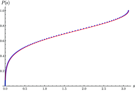
Figure 3: Cumulative spacings distribution $P(s)$ and its analytic approximation (50) (continuous red line) for $N=20$ and $m=2$.

A natural question in view of these results is to what extent the approximation (50) is applicable to other spin chains of HS type. For the PF chain of $A_{N}$ type, one can check that the spectrum satisfies conditions (i)–(iv) of this section, and in fact we have verified that (50) holds with remarkable accuracy in this case [35]. The situation is less clear for the original HS chain, whose spectrum is certainly not equispaced Finkel and González-López (2005). Nevertheless, our computations show that the formula (50) still fits the numerical data much better than our previous approximation (41), a fact clearly deserving further study. As an illustration, in Fig. 4 we compare the cumulative spacings distribution of the original HS chain with its approximations (41) and (50) for $N=25$ and $m=2$. It is apparent that the new expression (50) provides a more accurate approximation to the numerical data than the empiric formula (41) (their respective mean square errors are $1.8\times 10^{-5}$ and $5.8\times 10^{-4}$).

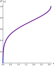
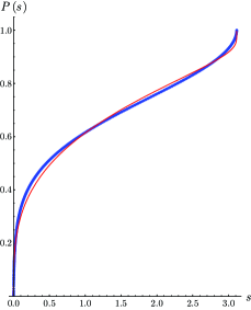
Figure 4: Cumulative spacings distribution $P(s)$ for the HS chain of $A_{N}$ type in the case of $N=25$ and $m=2$, compared to its continuous approximations (50) (left) and (41) (right). In both cases, the thin (red) line corresponds to the continuous approximation.

Appendix A Computation of $\mu$ and $\sigma^{2}$

In this appendix we shall compute in closed form the mean energy $\mu$ of the spin chain (1) and its standard deviation $\sigma^{2}$ as functions of the number of particles $N$ and internal degrees of freedom $m$.

In the first place, using the formulas for the traces of the operators $S_{ij}$, $\tilde{S}_{ij}$ and $S_{i}$ in Ref. Enciso et al. (2005) we easily obtain

$$\mu =\frac{\operatorname{tr}{\mathcal{H}}_{\epsilon}}{m^{N}}$$

$$=\Big{(}1+\frac{1}{m}\Big{)}\sum_{i\neq j}(h_{ij}+\tilde{h}_{ij})+\Big{(}1-\frac{\epsilon\mspace{1.0mu}p}{m}\Big{)}\sum_{i}h_{i}\,,$$ (51)

where $p$ is the parity of $m$ and

$$h_{ij}=(\xi_{i}-\xi_{j})^{-2}\,,\quad\tilde{h}_{ij}=(\xi_{i}+\xi_{j})^{-2}\,,\quad h_{i}=\beta\,\xi_{i}^{-2}\,.$$

The sums appearing in Eq. (51) can be expressed in terms of sums involving the zeros $y_{i}=\xi_{i}^{2}/2$, $1\leqslant i\leqslant N$, of the Laguerre polynomial $L_{N}^{\beta-1}$ as follows:

$$\sum_{i\neq j}(h_{ij}+\tilde{h}_{ij})=\sum_{i\neq j}\frac{2y_{i}}{(y_{i}-y_{j})^{2}}\,,\quad\sum_{i}h_{i}=\frac{\beta}{2}\sum_{i}\frac{1}{y_{i}}\,.$$ (52)

The latter sums can be easily computed using the following identities satisfied by the zeros $y_{i}$, which can be found in Ref. Ahmed (1978):

$$\sum_{j,j\neq i}\frac{2\,y_{i}}{y_{i}-y_{j}}=y_{i}-\beta\,,$$ (53)

$$\sum_{j,j\neq i}\frac{12\,y_{i}^{2}}{(y_{i}-y_{j})^{2}}=-y_{i}^{2}+2(2N+\beta)y_{i}-\beta(\beta+4)\,.$$ (54)

Indeed, from the first of these identities we easily obtain

$$\sum_{i}y_{i}=N(N+\beta-1)\,,\qquad\sum_{i}\frac{1}{y_{i}}=\frac{N}{\beta}\,,$$ (55)

so that, by Eq. (54),

$$\sum_{i\neq j}\frac{2\,y_{i}}{(y_{i}-y_{j})^{2}}=\frac{1}{6}\,\Big{(}-\sum_{i}y_{i}+2N(2N+\beta)\\ -\beta(\beta+4)\sum_{i}\frac{1}{y_{i}}\Big{)}=\frac{1}{2}\,N(N-1)\,.$$

Combining the last two equations with (51) and (52) we immediately arrive at Eq. (39) for the level density $\mu$.

Turning now to the standard deviation of the energy $\sigma^{2}$, from Eqs. (66)–(68) in Ref. Enciso et al. (2005) we have

$$\sigma^{2}=\frac{\operatorname{tr}{\mathcal{H}}_{\epsilon}^{2}}{m^{N}}-\mu^{2}=\Big{(}1-\frac{1}{m^{2}}\Big{)}\Big{(}2\sum_{i\neq j}\big{(}h_{ij}^{2}+\tilde{h}_{ij}^{2}\big{)}+\sum_{i}h_{i}^{2}\Big{)}\\ +\frac{4}{m^{2}}\,(1-p)\Big{(}\frac{1}{4}\sum_{i}h_{i}^{2}-\sum_{i\neq j}h_{ij}\tilde{h}_{ij}\Big{)}\,.$$ (56)

All of the sums appearing in the latter expression can be readily evaluated. Indeed, we have

$$\sum_{i}h_{i}^{2}=\frac{\beta^{2}}{4}\sum_{i}\frac{1}{y_{i}^{2}}=\frac{N(N+\beta)}{4(\beta+1)}$$ (57)

$$\sum_{i\neq j}h_{ij}\tilde{h}_{ij}=\frac{1}{4}\sum_{i\neq j}\frac{1}{(y_{i}-y_{j})^{2}}=\frac{N(N-1)}{16(\beta+1)}\,,$$ (58)

where we have used Eqs. (15) and (17) from Ref. Ahmed (1978). On the other hand,

$$\sum_{i\neq j}\big{(}h_{ij}^{2} +\tilde{h}_{ij}^{2}\big{)}=\frac{1}{2}\,\sum_{i\neq j}\frac{y_{i}^{2}+y_{j}^{2}+6y_{i}y_{j}}{(y_{i}-y_{j})^{4}}$$

$${}=2\sum_{i\neq j}\frac{y_{i}^{2}+y_{j}^{2}}{(y_{i}-y_{j})^{4}}-\frac{3}{2}\,\sum_{i\neq j}\frac{1}{(y_{i}-y_{j})^{2}}$$

$${}=4\sum_{i\neq j}\frac{y_{i}^{2}}{(y_{i}-y_{j})^{4}}-\frac{3N(N-1)}{8(\beta+1)}\,,$$ (59)

while from (Ahmed and Muldoon, 1983, Thm. 5.1) it follows that

$$720\sum_{i\neq j}\frac{y_{i}^{2}}{(y_{i}-y_{j})^{4}}=\sum_{i}y_{i}^{2}-4(2N+\beta)\sum_{i}y_{i}\\ +2N\big{(}8N^{2}+2(4N-1)\beta+3\beta^{2}\big{)}\\ -4(2N+\beta)(\beta^{2}-2\beta-18)\sum_{i}\frac{1}{y_{i}}\\ +\beta(\beta^{3}-4\beta^{2}-104\beta-144)\sum_{i}\frac{1}{y_{i}^{2}}\,.$$ (60)

All the sums in the right-hand side of the latter expression have already been evaluated in Eqs. (55) and (57), except the first one. In order to compute this sum, we multiply Eq. (53) by $y_{i}$ and sum over $i$, obtaining

$$\sum_{i\neq j}\frac{2y_{i}^{2}}{y_{i}-y_{j}} =\sum_{i\neq j}\frac{y_{i}^{2}-y_{j}^{2}}{y_{i}-y_{j}}=\sum_{i\neq j}(y_{i}+y_{j})$$

$$=2(N-1)\sum_{i}y_{i}=\sum_{i}y_{i}^{2}-\beta\sum_{i}y_{i}\,,$$

and hence, by Eq. (55),

$$\sum_{i}y_{i}^{2}=N(N+\beta-1)(2N+\beta-2)\,.$$ (61)

Substituting the value of the latter sum in Eq. (60) and using (55) and (57) we obtain

$$\sum_{i\neq j}\frac{y_{i}^{2}}{(y_{i}-y_{j})^{4}}=\frac{N(N-1)\big{(}(2N+5)\beta+2N+14\big{)}}{144(\beta+1)}\,.$$ (62)

Equation (40) now follows by inserting (57), (58) and (59)-(62) into Eq. (56).

Appendix B Computation of the minimum energy

In this appendix we shall obtain an explicit expression for the minimum energy ${\mathcal{E}}^{\epsilon}_{\mathrm{min}}$ of the spin chain (1). Our starting point is Eq. (7), which implies that ${\mathcal{E}}^{\epsilon}_{\mathrm{min}}$ is given by

$${\mathcal{E}}^{\epsilon}_{\mathrm{min}}=\lim_{a\to\infty}\frac{1}{a}\,\big{(}E^{\epsilon}_{\mathrm{min}}-E^{\mathrm{sc}}_{\mathrm{min}}\big{)}$$

in terms of the minimum energies $E^{\mathrm{sc}}_{\mathrm{min}}$ and $E^{\epsilon}_{\mathrm{min}}$ of the scalar and spin dynamical models (3) and (5), respectively. By the discussion in Section II (cf. Eq. (19)), ${\mathcal{E}}^{\epsilon}_{\mathrm{min}}$ is the minimum value of $|\mathbf{n}|$, where $\mathbf{n}$ is any multiindex compatible with conditions (i)–(iii) in the latter section. From these conditions it follows that the multiindex $\mathbf{n}$ minimizing $|\mathbf{n}|$ is given by

$$\mathbf{n}=\big{(}\overbrace{\vphantom{1}k,\dots,k}^{l}\,,\overbrace{\vphantom{1}k-1,\dots,k-1}^{l_{k-1}}\,,\dots,\overbrace{\vphantom{1}0,\dots,0}^{l_{0}}\big{)}\,,$$

where $0\leqslant l<l_{k}$ and $l_{i}$ is given by

$$l_{i}=\begin{cases}\frac{m}{2}\,,&m\text{ even}\\[2.84526pt] \frac{m+\epsilon}{2}\,,\quad&m\text{ odd and }i\text{ even}\\[2.84526pt] \frac{m-\epsilon}{2}\,,&m\text{ and }i\text{ odd\,.}\\ \end{cases}$$

In view of the above expression, it is convenient to treat separately the cases of even and odd $m$. For even $m$, we have $l_{i}=\frac{m}{2}$ for all $i$, so that

$$k=\lfloor 2N/m\rfloor\,,\qquad l=N\operatorname{mod}\frac{m}{2}\,,$$

and

$${\mathcal{E}}^{\epsilon}_{\mathrm{min}} =\frac{m}{2}\sum_{i=1}^{k-1}i+lk=\frac{m}{4}\,k(k-1)+lk$$

$$=\frac{N^{2}}{m}-\frac{N}{2}+\frac{l(m-2l)}{2m}\qquad\text{($m$ even)}\,.$$ (63)

Suppose now that $m$ is odd. If $k=2j$ is an even number, then $l_{0}=l_{2}=\dots=l_{2j-2}=\frac{m+\epsilon}{2}$, $l_{1}=l_{3}=\dots=l_{2j-1}=\frac{m-\epsilon}{2}$ and thus $N=jm+l$, so that

$$j=\lfloor N/m\rfloor\,,\qquad l=(N\operatorname{mod}m)<l_{2j}=\frac{m+\epsilon}{2}\,.$$

The minimum energy in this case is thus given by

$${\mathcal{E}}^{\epsilon}_{\mathrm{min}} =\frac{m+\epsilon}{2}\sum_{i=0}^{j-1}2i+\frac{m-\epsilon}{2}\sum_{i=0}^{j-1}(2i+1)+2jl$$

$$=mj(j-1)+j\,\frac{m-\epsilon}{2}+2jl$$

$$=\frac{N^{2}}{m}-\frac{N(m+\epsilon)}{2m}+\frac{l(m+\epsilon-2l)}{2m}\,.$$

On the other hand, if $k=2j+1$ is odd then $l_{0}=l_{2}=\dots=l_{2j}=\frac{m+\epsilon}{2}$, $l_{1}=l_{3}=\dots=l_{2j-1}=\frac{m-\epsilon}{2}$ and thus $N=jm+l+\frac{m+\epsilon}{2}$, with $0\leqslant l<l_{2j+1}=\frac{m-\epsilon}{2}$. Calling $l^{\prime}=l+\frac{m+\epsilon}{2}$ we have

$$j=\lfloor N/m\rfloor\,,\qquad l^{\prime}=(N\operatorname{mod}m)\geqslant\frac{m+\epsilon}{2}\,,$$

and

$${\mathcal{E}}^{\epsilon}_{\mathrm{min}} =\frac{m+\epsilon}{2}\sum_{i=0}^{j}2i+\frac{m-\epsilon}{2}\sum_{i=0}^{j-1}(2i+1)$$

$$\qquad+(2j+1)\Big{(}l^{\prime}-\frac{m+\epsilon}{2}\Big{)}$$

$$=mj(j-1)+j\,\frac{m-\epsilon}{2}+2jl^{\prime}+l^{\prime}-\frac{m+\epsilon}{2}$$

$$=\frac{N^{2}}{m}-\frac{N(m+\epsilon)}{2m}+\frac{(l-m)(m+\epsilon-2l)}{2m}\,.$$

Hence we can express the minimum energy for odd $m$ in a unified way as

$${\mathcal{E}}^{\epsilon}_{\mathrm{min}} =\frac{N^{2}}{m}-\frac{N(m+\epsilon)}{2m}+\frac{1}{2m}\,\big{(}l-m\,\theta(2l-m-\epsilon)\big{)}$$

$$\quad{\times}(m+\epsilon-2l)\qquad\qquad\qquad\text{($m$ odd)}\,,$$ (64)

where

$$l=N\operatorname{mod}m$$

and $\theta(x)=1$ for $x\geqslant 0$ and $0$ otherwise.