Modeling interaction of trading volume in financial dynamics
Abstract
A dynamic herding model with interactions of trading volumes is introduced. At time , an agent trades with a probability, which depends on the ratio of the total trading volume at time to its own trading volume at its last trade. The price return is determined by the volume imbalance and number of trades. The model successfully reproduces the power-law distributions of the trading volume, number of trades and price return, and their relations. Moreover, the generated time series are long-range correlated. We demonstrate that the results are rather robust, and do not depend on the particular form of the trading probability.
keywords:
Econophysics; Scaling laws; Complex systemsPACS:
89.65.Gh, 89.75.Da, 89.75.-k1 Introduction
In statistical analysis of financial markets, much attention has been drawn to the study of the stock prices [1, 2, 3, 4, 5, 6, 7, 8, 9, 10, 11, 12, 13]. Denoting as the price of a given stock or financial index, the price return is defined as the change of the logarithmic price in a time interval , i.e., . A power-law tail with an exponent is found in the cumulative probability distribution of price returns [6, 7, 8], which indicates that the large price fluctuation is more common than one might naively expect. Another important statistical property basically observed in financial markets is the long-range correlation of the volatility which is simply defined as the magnitude of the price return [9, 10]. Many efforts have been devoted to the understanding of the financial markets along this direction, with both phenomenological analysis and microscopic multi-agent models [3, 6, 7, 9, 14, 15, 16, 17, 18, 19, 20, 21, 22].
Recent empirical studies show that the trading volume is highly correlated with the price return and volatility [8, 23, 24, 25], and this confirms the famous saying that it takes trading volume to move stock prices. A positive linear correlation is revealed based on the data analysis at time scales large than one minute [26, 27, 28]. For the high-frequency data at microscopic transaction level, the volume-return relation follows a scaling behavior. Lillo et al. found a mater curve with scaling form using the Trade and Quote database of US stocks [29], and the scaling function is found to be a power-law form for large volumes. Lim and Zhou found similar scaling behavior in Australian and Chinese stocks [30, 31]. Due to the significant importance of the trading volume, its statistical properties is worthy of being carefully analyzed.
Interestingly the cumulative probability distributions of the trading volume as well as the number of trades also show power-law behaviors, and the corresponding exponents are reported to be and respectively [7, 8, 25]. To understand the power-law distributions of the trading volume and number of trades, and their possible relations with the distribution of price returns, an effective theory is promoted by Gabaix et al [8], based on the empirical power-law relation between the large trading volume and the large price return. Instead, from the phenomenological analysis of the order book data, Farmer and Weber et al. suggest that large price movements are driven by the fluctuation in liquidity [32, 33], e.g., variations in the response to changes in supply and demand, and the low density of limit orders, etc. In fact, it is highly nontrivial to offer a complete answer, how large price movements occur. Nevertheless, it remains very important to fully understand the statistical properties of the financial fluctuations, such as the power-law distributions of different quantities, and their relations, as well as the long-range time correlations.
In this paper we develop a multi-agent model of trading activity, aiming at a full understanding of the statistical properties of the financial fluctuations including the power-law distributions of the price return, trading volume and number of trades and the long-range time correlation of the volatility. In the literature, some stochastic models of trading activity, typically at the phenomenological level, have been analyzed for this purpose [34, 35, 36]. Certain aspects of the financial fluctuations could be reproduced. A multiplicative stochastic model of the time interval between two successive trades, for example, is able to reproduce the statistical properties of the number of trades [34], but does not refer to the relation with the power-law distributions of the price return and trading volume. In the present paper, we construct our model based on the microscopic structure and interactions, to capture fundamental mechanisms in the financial dynamics.
The paper is organized as follows. In Sec. II, the dynamic herding model with interactions of trading volumes is introduced. In Sec. III, numerical results of the model are presented. Sec. IV contains the conclusion.
2 Model definition
The concept of percolating or herding is important in describing the financial markets [16, 18, 37]. The dynamic version of the static percolation model, the so-called EZ herding model, shows certain attractive features [18], e.g., the herding structure is dynamically generated in a simple but robust way. The EZ herding model captures the power-law distribution of the price return, but the volatility is short-range correlated in time. To achieve the long-range time correlation of the volatility, a feed-back interaction should be introduced [20, 38]. Up to now, however, it is still far from realistic and harmonic. For example, only the volatility is concerned. The trading volume and number of trades have not been touched. The price return is calculated from the volatility with random signs, and this should not describe the realistic financial dynamics.
In this section, we develop a dynamic herding model including the price return, trading volume, and number of trades. In fact, it is not easy to build such a model. We have probed many possible variations of the microscopic structure and interaction, and finally come to the present form.
2.1 Standard EZ herding model
To start, let us first consider the EZ herding model. The system consists of agents, which form clusters during dynamic evolution. Initially, each agent is a cluster. The dynamics evolves in the following way:
(1) At a time step , select an agent (and thus its cluster) at random.
(2) With a probability , remains inactive in trading, and select another agent randomly. If and are in different clusters, combine the two clusters into one.
(3) With a probability , becomes active and makes a trade. Then all agents in the cluster follow. After that, this cluster is broken into a state that each agent is a separate cluster. The size of this cluster is recorded as .
Here the probability is a constant, and controls the dynamic evolution. Since one does not define buying or selling of the trade, only the magnitude of the price return defined as is essentially generated. The step (2) represents transmission of information. Considering the time between two actions as the time unit, is the rate of transmission of information. If is small, for example, transmission of information is fast, and agents tend to form larger clusters and act collectively. Numerical simulations [18] show that for a certain value of , the probability distribution obeys a power law.
2.2 Herding model interacted with trading volume
However, the EZ herding model does not exhibit the long-range time correlation of the volatility. Furthermore, we need to include the price return, trading volume and number of trades [8, 23, 25]. Therefore, we assume that each agent trades with an individual trading volume . Denoting buying and selling with and respectively, all agents in a cluster are given a same trade sign . Initially, each agent with is a cluster, and randomly selects a trade sign . The total trading volume is set to . We construct the dynamics as following:
(1) At a time step , select an agent (and thus its cluster) at random, and calculate the trading probability
| (1) |
Here is the trading volume of at its last trade, is the total trading volume at , and the parameter is a positive value.
(2) With a probability , the agent remains inactive in trading, and select another agent randomly. If and are in different clusters, combine the two clusters into one. The trade sign of the new cluster is taken to be that of the larger cluster of the previous two.
(3) With a probability , all agents in the cluster which belongs to and another randomly selected cluster become active, and make trades according to their trade signs. After that, these two clusters are broken into a state that each agent is a separate cluster with a trade sign selected randomly.
Our plausible observation is that if an agent is collecting much information, i.e., with a small , it may perform a large trade. Therefore, we assume to be the trading volume of the agent . Then is the total trading volume, with the sum over the two active clusters. Let denote the number of agents in the two active clusters, we define it as the number of trades.
To determine the price return, we need more careful consideration. Empirical studies show that the trading volume seems to have a square root impact on the price return, and the price return saturates at extremely large trading volumes [8, 23]. Further, the correlation between the price return and trading volume is largely due to the number of trades [25, 39].Following the square root price impact function, we assume that the price return is determined by the volume imbalance and the number of trades. The volume imbalance reflects the difference between supply and demand [32, 33]. Quantitatively, we define the price return
| (2) |
The parameter is taken to be a large positive value, such that at relatively small , and at extremely large .
The key ingredient in our model is the time-dependent probability . In Eq. (1), we assume that depends on the ratio of the total trading volume at time to its individual trading volume at its last trade. In financial markets, a large trading volume is usually accompanied by the strong fluctuation of the price return [8, 23, 25]. This inversely leads to large trading volumes in next time steps. Therefore, is taken to be inversely proportional to the trading volume . If is large, transmission of information is fast, the probability of combining two clusters is high, then the number of the trades increases on average, and finally leads to large trading volumes. Such a dynamic feed-back interaction of the trading volume essentially generates the long-range time correlation of the volatility. On the other hand, is taken to be proportional to the individual trading volume at its last trade, based on the empirical assumption that an agent with a large trading volume in its last trade may be more active in trading in next time steps. Further, the thermodynamic limit is well defined due to the ratio in Eq. (1).
3 Simulation results
3.1 Probability distribution function
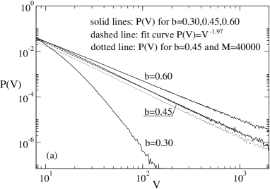
In our model, the only tunable parameter is . In calculating the price return, we fix the value . For each value of , we take an average over iterations, after iterations for equilibration. To detect the finite size effect, we perform extensive simulations with different total numbers of agents, and find that the results become stable for as shown in Fig. 1 (a). Therefore, we report the results with .
From empirical studies of the stock time series, the probability distribution of the trading volume obeys a power law
| (3) |
with , while that of the number of trades obeys
| (4) |
with . The exponents of these two power-law distributions appear to have an approximate relation [8] .
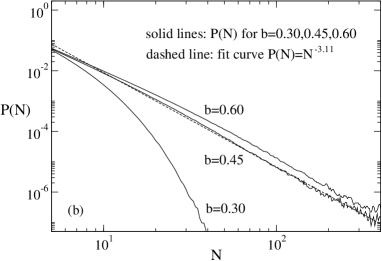
The probability distributions of the trading volume and number of
trades in our model are carefully investigated. In Fig. 1 (a) and (b), and are plotted
for in log-log scale. For a small , e.g.,
, and decay rapidly, and do not show a
power-law behavior. As increases, both and show a
power-law behavior at , at least in two orders of magnitude.
In this sense, the system exhibits a ’cross-over’ behavior. Fitting
the curves with the power laws in Eqs.(3) and (4),
we estimate and . These values of the
exponents are consistent with the approximate relation . For , remains a power-law behavior
in a broad range of , but the exponent changes with
and becomes smaller. On the other hand, deviates from a
power-law behavior up to a medium value , while a power-law tail
is still kept with an exponent approximately the same as
that at . In Fig. 1, the curves
for are displayed.
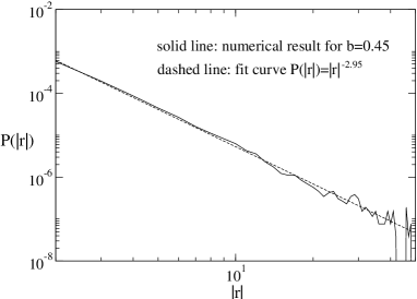
It is well known from the empirical analysis that the probability distribution of the price return exhibits a power-law tail
| (5) |
with [7]. In Fig. 2, the probability distribution of the price return of our model is plotted for in log-log scale. The curve can be nicely fitted with a power law, and the exponent is estimated to be , close to . In summary, our dynamic herding model at captures the power-law distributions of the trading volume, number of trades and price return. The corresponding exponents of these power-law distributions follow an approximate relation . This is in agreement with that of the real markets reported in Ref. [8], though the exponents themselves are slightly different.
The specific form of is not very important. Other functions may also work, if their behaviors are similar to that in Eq. (1). To verify this we also study the model with another with a form
| (6) |
where and are two positive parameters. We remain the inverse relation between and the ratio , thus makes it behave similar to Eq. (1). An important characteristic of this model is the simple relation between the trading volume and trading probability. It indicates that are the dynamic variables, interact each other through the trading probability , and evolve according to Eq. (6).
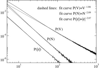
We study the probability distributions of trading volume, number of
trades and price return for the model with defined in
Eq. (6). To make the probability fixed between
and , we set . By adjusting the parameter , one
observes a ’cross-over’ behavior similar to the model with
defined in Eq. (1): for small , no
power-law behavior is observed, while for large power-law
behavior occurs. In Fig. 3, power behaviors of
, and for a large are plotted. By
fitting the slopes of these curves, we estimate ,
and . These exponents display a
relation also consistent with
that of the real markets.
3.2 Auto-correlation function
The long-range time correlation of the volatility is another important feature of the financial markets. Let us define the the auto-correlation function of the magnitude of the price return as
| (7) |
where represents the average over the time . From the empirical analysis, it obeys a power law,
| (8) |
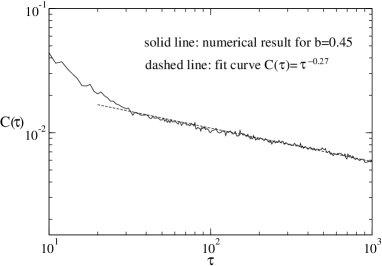
We calculate of the model with defined in
Eq. (1), and observe that a power-law behavior is achieved
only when is in the very neighborhood of . In Fig. 4 (b), is plotted for in
log-log scale. The curve can be nicely fitted by a power law,
indicating a long-range time correlation of the volatility. The
exponent is estimated to be , very close to that of
the real markets. This improves the result in a naive
model [38]. A power law with an
exponent (not shown in figure) is also observed in
of the model with another defined in Eq. (6), but
with a reactively bigger fluctuation.
In our model, a large price movement is induced by a large volume imbalance and a large number of trades due to the price dynamics defined in Eq. (2). This may occur when large clusters exist in the system. Large clusters are formed after agents are active in collecting information for a period of time. However, a single large trading volume does not necessarily lead to a large price movement.
4 Conclusion
We introduce a dynamic herding model with interactions of trading volumes. At time , each agent trades with a probability as a linear function of the ratio of the total trading volume at time to its own trading volume at its last trade. Agents are endowed with trade signs denoting buying and selling, and the price return is determined by the volume imbalance and number of trades. We find that at a threshold , our model reproduces the power-law distributions of the trading volume, number of trades and price return, and more importantly, the approximate relation . The generated volatilities are long-range correlated in time. We also investigate the model with another exponential form of which remains its inverse relation with the ratio , and similar power-law behaviors and long-range correlation are observed. This indicates the robustness of our model.
By simulating the agents’ reactions to the market information through the interactions between their individual trading volumes and the total trading volumes, the model can explain the power-law behaviors of the trading volume, number of trades and price return, and their relations. We believe that our model captures certain essences of the financial markets. Further works should include understanding of the Leverage and anti-Leverage effects in western and Chinese financial markets [40, 41, 42, 43], and more general interactions between the price return, trading volume and number of trades, etc.
Acknowledgments:
This work was supported in part by NNSF (China) under grant Nos. 10325520, 70371069 and 10905023, and ”Chen Guang” project sponsored by Shanghai Municipal Education Commission and Shanghai Education Development Foundation under grant No. 2008CG37.
References
- [1] B. B. Mandelbrot, The variation of certain speculative prices, J. Business 36 (1963) 394–419.
- [2] E. F. Fama, The behavior of stock market prices, J. Business 38 (1) (1965) 34–105.
- [3] R. N. Mantegna, H. E. Stanley, Scaling behaviour in the dynamics of an economic index, Nature 376 (1995) 46–49.
- [4] T. Lux, The Stable Paretian Hypothesis and the Frequency of Large Returns: An Examination of Major German Stocks, Appl. Financ. Econ. 6 (1996) 463–475.
- [5] S. Ghashghaie, W. Breymann, J. Peinke, P. Talkner, Y. Dodge, Turbulent cascades in foreign exchange markets, Nature 381 (1996) 767–770.
- [6] V. Plerou, P. Gopikrishnan, L. A. N. Amaral, M. Meyer, H. E. Stanley, Scaling of the distribution of price fluctuations of individual companies, Phys. Rev. E 60 (1999) 6519–6529.
- [7] V. Plerou, P. Gopikrishnan, L. A. N. Amaral, X. Gabaix, H. E. Stanley, Economic fluctuations and anomalous diffusion, Phys. Rev. E 62 (2000) R3023–R3026.
- [8] X. Gabaix, P. Gopikrishnan, V. Plerou, H. E. Stanley, A theory of power-law distributions in financial market fluctuations, Nature 423 (2003) 267–270.
- [9] I. Giardina, J. Bouchaud, M. Mézard, Microscopic models for long ranged volatility correlations, Physica A 299 (2001) 28–39.
- [10] Y.-H. Liu, P. Gopikrishnan, P. Cizeau, M. Meyer, C.-K. Peng, H. E. Stanley, Statistical properties of the volatility of price fluctuations, Phys. Rev. E 60 (1999) 1390–1400.
- [11] R. N. Mantegna, H. E. Stanley, An Introduction to Econophysics: Correlations and Complexity in Finance, Cambridge University Press, Cambridge, 2000.
- [12] J.-P. Bouchaud, M. Potters, Theory of Financial Risks: From Statistical Physics to Risk Management, Cambridge University Press, Cambridge, 2000.
- [13] D. Sornette, Why Stock Markets Crash: Critical Events in Complex Financial Systems, Princeton University Press, Princeton, 2003.
- [14] F. Ren, B. Zheng, Generalized persistence probability in a dynamic economic index, Phys. Lett. A 313 (2003) 312–315.
- [15] D. Challet, Y.-C. Zhang, Emergence of cooperation and organization in an evolutionary game, Physica A 246 (1997) 407–418.
- [16] D. Stauffer, D. Sornette, Self-organized percolation model for stock market fluctuations, Physica A 271 (1999) 496–506.
- [17] J.-F. Muzy, J. Delour, E. Bacry, Modelling fluctuations of financial time series: from cascade process to stochastic volatility model , Eur. Phys. J. B 17 (2000) 537–548.
- [18] V. M. Eguíluz, M. G. Zimmermann, Transmission of information and herd behavior: An application to financial markets, Phys. Rev. Lett. 85 (2000) 5659–5662.
- [19] A. Krawiecki, J. A. Holyst, D. Helbing, Volatility clustering and scaling for financial time series due to attractor bubbling, Phys. Rev. Lett. 89 (2002) 158701.
- [20] B. Zheng, T. Qiu, F. Ren, Two-phase phenomena, minority games, and herding models, Phys. Rev. E 69 (2004) 046115.
- [21] F. Ren, B. Zheng, T. Qiu, S. Trimper, Minority games with score-dependent and agent-dependent payoffs, Phys. Rev. E 74 (2006) 041111.
- [22] G.-F. Gu, W.-X. Zhou, Emergence of long memory in stock volatilities from a modified Mike-Farmer model, EPL 86 (2009) 48002. doi:10.1209/0295-5075/86/48002.
- [23] J. Hasbrouck, Measuring the information content of stock trades, J. Financ. 46 (1991) 179–207.
- [24] J. M. Karpoff, The relation between price changes and trading volume: A survey, J. Financ. Quant. Anal. 22 (1987) 109–126.
- [25] P. Gopikrishnan, V. Plerou, X. Gabaix, H. E. Stanley, Statistical properties of share volume traded in financial markets, Phys. Rev. E 62 (2000) R4493–R4496.
- [26] R. A. Wood, T. H. McInish, J. K. Ord, An investigation of transactions data for NYSE stocks, J. Financ. 40 (1985) 723–739.
- [27] A. R. Gallant, P. E. Rossi, G. Tauchen, Stock prices and volume, Rev. Financ. Stud. 5 (1992) 199–242.
- [28] K. Saatcioglu, L. T. Starks, The stock price-volume relationship in emerging stock markets: the case of Latin America, Int. J. Forecast. 14 (1998) 215–225.
- [29] F. Lillo, J. D. Farmer, R. Mantegna, Master curve for price impact function, Nature 421 (2003) 129–130.
- [30] M. Lim, R. Coggins, The immediate price impact of trades on the Australian Stock Exchange, Quant. Financ. 5 (2005) 365–377.
- [31] W.-X. Zhou, Universal price impact functions of individual trades in an order-driven market, arXiv: 0708.3198v2 (2007).
- [32] J. D. Farmer, L. Gillemot, F. Lillo, S. Mike, A. Sen, What really causes large price changes?, Quant. Financ. 4 (2004) 383–397.
- [33] P. Weber, B. Rosenow, Large stock price changes: Volume or liquidity?, Quant. Financ. 6 (2006) 7–14.
- [34] Gontis-Kaulakys-2004-PA, Multiplicative point process as a model of trading activity, Physica A 343 (2004) 505–514.
- [35] A. H. Sato, Explanation of power law behavior of autoregressive conditional duration processes based on the random multiplicative process, Phys. Rev. E 69 (2004) 047101.
- [36] S. Das, A Learning Market-Maker in the Glosten-Milgrom Model, Quant. Financ. 5 (2005) 169.
- [37] R. Cont, J.-P. Bouchaud, Herd behavior and aggregate fluctuations in financial markets, Macroecon. Dyn. 4 (2000) 170–196.
- [38] B. Zheng, F. Ren, S. Trimper, D.-F. Zheng, A generalized dynamic herding model with feed-back interactions, Physica A 343 (2004) 653–661.
- [39] V. Plerou, P. Gopikrishnan, X. Gabaix, H. E. Stanley, Quantifying stock-price response to demand fluctuations, Phys. Rev. E 66 (2002) 027104. doi:10.1103/PhysRevE.66.027104.
- [40] F. Ren, B. Zheng, H. Lin, L. Wen, S. Trimper, Persistence probabilities of the German DAX and Shanghai index, Physica A 350 (2005) 439.
- [41] T. Qiu, B. Zheng, F. Ren, S. Trimper, Return-volatility correlation in financial dynamics, Phys. Rev. E 73 (2006) 065103(R).
- [42] T. Qiu, B. Zheng, F. Ren, S. Trimper, Statistical properties of German Dax and Chinese indices, Physica A 378 (2007) 387–398.
- [43] J. Shen, B. Zheng, On return-volatility correlation in financial dynamics, Europhys. Lett. 88 (2009) 28003.