Abstract

We analyze the quark-gluon induced process $ug\to\tilde{d}\tilde{\chi}_{i}^{+}$, including the one loop electroweak (EW) effects in the minimal supersymmetric model (MSSM). This process is dominated by $\tilde{d}_{L}$-production and is determined by four helicity amplitudes, three of which are violating helicity conservation, and another one which respects it and is logarithmically enhanced at high energy. Combining this $ug\to\tilde{d}_{L}\tilde{\chi}_{i}^{+}$ analysis with a corresponding one for $ug\to dW^{+}$, we obtain simple approximate relations between the two processes, testing the MSSM structure at the amplitude and the cross section levels. These relations become exact at asymptotic energies and, provided the SUSY scale is not too heavy, they may be approximately correct at LHC energies also. In addition to these, we study the 1loop EW corrections to the inclusive $\tilde{d}\tilde{\chi}_{i}^{+}$ production at LHC, presenting as examples, the $p_{T}$ and angular distributions. Comparing these to the corresponding predictions for $W$+jet production derived earlier, provides an accurate test of the supersymmetric assignments.

PACS numbers: 12.15.-y, 12.15.-Lk, 14.70.Fm, 14.80.Ly

1 Introduction

In a previous paper we have shown that the 1loop virtual SUSY EW effects in the process $ug\to dW^{+}$, present a number of remarkable properties [1]. Among them, is the role of SUSY in ensuring the validity of Helicity Conservation (HC) for any two-body process at high energy, to all orders in perturbation theory [2]. By this we mean the fact that at very high energies and fixed angles, the only surviving two-body amplitudes are those where the sum of the initial particle helicities equal to the sum of the final particle helicities [2]. According to HC, these are the only amplitudes that could possibly contribute at asymptotic energies, and in fact receive the logarithmic enhancements extensively studied in [3] and [4]. All the rest must vanish in this limit.

These results raised several questions concerning the deeper reasons for the validity of HC, and whether terms involving ratios of masses could possibly violate it. Such questions called for further studies of various explicit processes [1]. Particular among them, are processes involving heavy SUSY-particles in the final state, where establishing of HC is expected to be delayed.

Along these lines of thought, we present here an analysis of the process $ug\to\tilde{d}_{L}\tilde{\chi}_{i}^{+}$, which starts from the same initial state as $ug\to dW^{+}$, but its final state involves SUSY partners of $dW^{+}$. Such a study could provide insights into the SUSY implications, which of course become clearest at the highest energy.

Denoting the helicities and momenta of the incoming and outgoing particles in the above process as

$$u(p_{u},\lambda_{u})+g(p_{g},\lambda_{g})\to\tilde{d}_{L}(p_{\tilde{d}})+\tilde{\chi}_{i}^{+}(p_{\tilde{\chi}},\lambda_{\tilde{\chi}})~{}~{},$$ (1)

we write the corresponding helicity amplitudes as $F^{\tilde{\chi}}_{\lambda_{u}\lambda_{g}\lambda_{\tilde{\chi}}}$.

At Born level, these amplitudes are determined by the two diagrams in Fig.1a, characterized by a $u$-quark exchange in the s-channel, and a $\tilde{d}_{L}$-squark exchange in the u-channel. Because of the negligible u and d quark masses, the charginos couple only through their pure gaugino components, so that the appearance of a right-handed $\tilde{d}_{R}$-squark in the final state is very strongly suppressed. Moreover, the incoming u-quark must always be left-handed, with $\lambda_{u}=-1/2$. The mixing in the ($\tilde{d}_{L},\tilde{d}_{R}$) system is also generally negligible, since it behaves like $m_{d}(A_{d}-\mu\tan\beta)/M_{q}^{2}$, with $M_{q}$ being the soft SUSY breaking mass term. Only for extremely large $\mu\tan\beta$ it may acquire some relevance, which can easily be taken into account at the end, when discussing the numerical results. Therefore, we neglect ($\tilde{d}_{L},\tilde{d}_{R}$)-mixing in the theoretical part of this work.

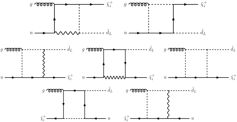
Figure 2: Independent box diagrams used for $ug\to\tilde{d}_{L}\tilde{\chi}_{i}^{+}$. Full, broken and wavy lines describe respectively fermionic, scalar and gauge particles.

These properties remain true also at the 1loop EW level, as it can be seen from the relevant diagrams, shown in Figs.1 and 2. So, only four independent helicity amplitudes remain for the process (1), corresponding to $\lambda_{g}=\pm 1$ and $\lambda_{\tilde{\chi}}=\pm 1/2$; namely

$$F^{\tilde{\chi}}_{---}~{}~{},~{}~{}F^{\tilde{\chi}}_{--+}~{}~{},~{}~{}F^{\tilde{\chi}}_{-+-}~{}~{},~{}~{}F^{\tilde{\chi}}_{-++}~{}~{}.$$ (2)

The HC rule would then predict that at fixed angles, and energies much larger than all SUSY masses, the first three amplitudes $F^{\tilde{\chi}}_{---}$, $F^{\tilde{\chi}}_{--+}$ and $F^{\tilde{\chi}}_{-+-}$ should all vanish, most often like $M^{2}/s$, with $M$ being some ”average” SUSY mass [2]. Only the last amplitude $F^{\tilde{\chi}}_{-++}$, which respects HC, could possibly have a non-vanishing, logarithmically increasing limit [2, 3, 4].

To see this explicitly, we make a complete computation of the one loop electroweak contributions to the $ug\to\tilde{d}_{L}\tilde{\chi}_{i}^{+}$ helicity amplitudes. Our results are contained in a FORTRAN code, available at the site [5], which calculates all four helicity amplitudes of (2), in any MSSM with real parameters.

Using these results, we then present the angular and energy dependance of each helicity amplitude, for three benchmark cases covering light, medium and high SUSY masses. This way, we try to illustrate how HC establishes itself at high energies. In particular, how the corrections to the leading amplitude $F^{i}_{-++}$ match the high energy leading logs approximation; and how the individual, relatively large contributions to the helicity violating amplitudes, cancel each other at high energies, and produce vanishing results, in accordance to the HC rule.

We next compare these results to those for $ug\to dW$ obtained in [1]. Denoting the $ug\to dW$ 1loop helicity amplitudes as $F^{W}_{\lambda_{u}\lambda_{g}\lambda_{d}\lambda_{W}}$, and comparing the leading helicity conserving amplitudes $F^{W}_{----}$ and $F^{W}_{-+-+}$, with the above $F^{\tilde{\chi}}_{-++}$ for $\tilde{d}_{L}\tilde{\chi}^{+}_{i}$-production, we derive relations which test the supersymmetric connection between the two processes at asymptotic energies. These are subsequently transformed to simple relations among the differential cross sections for $ug\to\tilde{d}_{L}\tilde{\chi}_{i}^{+}$ and $ug\to dW^{+}$, which should be very good asymptotically, but may be ”not bad” for LHC energies also.

Studying experimentally these SUSY $\sigma$-relations, could teach us how the asymptotic SUSY properties are modified at LHC energies by ”constant” terms; i.e. terms which do not depend on energy, but may depend on the scattering angle and the SUSY masses and couplings.

Independently of these, we also study the exact one-loop EW corrections to $\tilde{d}_{L}\tilde{\chi}_{i}^{+}$-production at LHC, and compare it to the corresponding study for $W$+jet production [1]. In particular, we study the angular and transverse momentum distributions. Such a study provides a test of whether the identification of two ”candidate particles” possibly pair-produced at LHC, as a $\tilde{d}_{L}$ and a $\tilde{\chi}_{i}^{+}$, is consistent.

The contents of the paper are: In Sect.2, the Born and the 1oop EW contributions to the $ug\to\tilde{d}_{L}\tilde{\chi}^{+}_{i}$ helicity amplitudes are presented, as well as the FORTRAN code. In Sect.3, the high energy properties of the $ug\to\tilde{d}_{L}\tilde{\chi}^{+}_{i}$ and $ug\to dW^{+}$ amplitudes are given, together with their SUSY relations. The corresponding numerical results appear in Sect.4, while in Sect.5 we give the EW contribution to the LHC $\tilde{d}_{L}\tilde{\chi}^{+}_{i}$-production. Sect.6 contains our conclusions and outlook.

2 The one loop electroweak amplitudes for $ug\to\tilde{d}_{L}\tilde{\chi}^{+}_{i}$

Defining the momenta and helicities of the incoming and outgoing particles as indicated in (1), and using also

$$s=(p_{u}+p_{g})^{2}~{}~{},~{}~{}u=(p_{\tilde{d}}-p_{g})^{2}=(p_{u}-p_{\tilde{\chi}})^{2}~{}~{},~{}~{}t=(p_{g}-p_{\tilde{\chi}})^{2}=(p_{u}-p_{\tilde{d}})^{2}~{}~{},$$ (3)

we express the initial and final energies and momenta as

$$E_{u}=E_{g}=p_{u}=p_{g}=p={\sqrt{s}\over 2}~{}~{},~{}~{}$$

$$E_{\tilde{\chi}}={s+m^{2}_{\tilde{\chi}}-m^{2}_{\tilde{d}}\over 2\sqrt{s}}~{}~{},~{}~{}E_{\tilde{d}}={s-m^{2}_{\tilde{\chi}}+m^{2}_{\tilde{d}}\over 2\sqrt{s}}~{},$$

$$p^{\prime}=p_{\tilde{d}}=p_{\tilde{\chi}}=\sqrt{E^{2}_{\tilde{\chi}}-m^{2}_{\tilde{\chi}}}=\frac{\sqrt{[s-(m_{\tilde{\chi}}+m_{\tilde{d}})^{2}][s-(m_{\tilde{\chi}}-m_{\tilde{d}})^{2}]}}{2\sqrt{s}}~{},$$ (4)

where the mass of the $u$-quark has been ignored. For later use we also give the kinematical variables

$$R=\sqrt{E_{u}(E_{\tilde{\chi}}+m_{\tilde{\chi}})}={1\over 2}\sqrt{(\sqrt{s}+m_{\tilde{\chi}})^{2}-m^{2}_{\tilde{d}}}~{},$$

$$\beta^{\prime}_{\tilde{\chi}}={2p^{\prime}\over\sqrt{s}}~{}~{},~{}~{}~{}r_{u}={p\over E_{u}}=1~{}~{}~{},~{}~{}r_{\tilde{\chi}}={p^{\prime}\over E_{\tilde{\chi}}+m_{\tilde{\chi}}}~{},$$ (5)

while the c.m. scattering angle and transverse momentum are defined through

$$u=\frac{1}{2}(m_{\tilde{\chi}}^{2}+m_{\tilde{d}}^{2}-s)-\frac{1}{2}\sqrt{[s-(m_{\tilde{\chi}}+m_{\tilde{d}})^{2}][s-(m_{\tilde{\chi}}-m_{\tilde{d}})^{2}]}\cos\theta~{},$$

$$t=\frac{1}{2}(m_{\tilde{\chi}}^{2}+m_{\tilde{d}}^{2}-s)+\frac{1}{2}\sqrt{[s-(m_{\tilde{\chi}}+m_{\tilde{d}})^{2}][s-(m_{\tilde{\chi}}-m_{\tilde{d}})^{2}]}\cos\theta~{},$$ (6)

$$\cos\theta=\sqrt{1-\frac{p_{T}^{2}}{p^{\prime 2}}}~{}~{}~{}~{},~{}~{}~{}~{}|t-u|=s\beta^{\prime}_{\tilde{\chi}}\sqrt{1-\frac{p_{T}^{2}}{p^{\prime 2}}}~{}~{}.$$ (7)

The Born contribution to $ug\to\tilde{d}_{L}\tilde{\chi}^{+}_{i}$, may be written as

$$F^{\tilde{\chi},\rm~{}Born}_{-\lambda_{g}\lambda_{\tilde{\chi}}}=F^{\tilde{\chi},~{}s-{\rm Born}}_{-\lambda_{g}\lambda_{\tilde{\chi}}}+F^{\tilde{\chi},~{}u-{\rm Born}}_{-\lambda_{g}\lambda_{\tilde{\chi}}}~{}~{},$$ (8)

with the two terms

$$F^{\tilde{\chi},~{}s-{\rm Born}}_{-\lambda_{g}\lambda_{\tilde{\chi}}} = -\left(\frac{\lambda^{a}}{2}\right){g_{s}A^{L}_{i}(\tilde{d}_{L})\over 2s}R\sqrt{2s}(1-\lambda_{g})(1+2\lambda_{\tilde{\chi}}r_{\tilde{\chi}})\left[\sin{\theta\over 2}\delta_{\lambda_{\tilde{\chi}},+}-\cos{\theta\over 2}\delta_{\lambda_{\tilde{\chi}},-}\right]~{},$$ (9)

$$F^{\tilde{\chi},~{}u-{\rm Born}}_{-\lambda_{g}\lambda_{\tilde{\chi}}} = \left(\frac{\lambda^{a}}{2}\right){g_{s}A^{L}_{i}(\tilde{d}_{L})\over u-m^{2}_{\tilde{d}_{L}}}R\sqrt{2}\lambda_{g}p^{\prime}\sin\theta(1+2\lambda_{\tilde{\chi}}r_{\tilde{\chi}})\left[\cos{\theta\over 2}\delta_{\lambda_{\tilde{\chi}},+}+\sin{\theta\over 2}\delta_{\lambda_{\tilde{\chi}},-}\right]~{},$$ (10)

arising from the two diagrams in Fig.1a. The $u$-quark exchange diagram is responsible for (9), while (10) comes from $\tilde{d}_{L}$-exchange in the u-channel. The overall factor $\lambda^{a}/2$ describes the color matrices acting between the initial $u$-quark and the final $\tilde{d}_{L}$-squark, while $g_{s}$ is the QCD coupling. Finally,

$$A^{L}_{i}(\tilde{d}_{L})=-\frac{e}{s_{W}}Z^{-}_{1i}~{}~{},$$ (11)

expresses the $u\tilde{d}_{L}$-coupling of the produced chargino, in terms of its gaugino-higgsino mixing matrix $Z^{-}$, in the notation of [6].

The 1loop EW corrections arise from the diagrams in Figs.1b,c and 2, to which we should also add the counter terms (c.t.) induced by the $A^{L}_{i}(\tilde{d}_{L})$-renormalization, and the self energy (s.e.) corrections to the external and internal lines of the tree diagrams in Fig.1a.

We first discuss these c.t. and s.e. energy corrections, which are simply expressed by modifying the Born contribution (8, 9, 10) as

$$F^{\tilde{\chi},~{}s-{\rm Born}}_{-\lambda_{g}\lambda_{\tilde{\chi}}} \to F^{\tilde{\chi},~{}s-{\rm Born}}_{-\lambda_{g}\lambda_{\tilde{\chi}}}\Bigg{\{}1+\delta Z^{u}_{L}+{1\over 2}\Big{[}\delta Z^{u}_{L}+\delta Z_{\tilde{d}_{L}}$$ (12)

$$+{1\over A^{L}_{i}(\tilde{d}_{L})}\sum_{j}A^{L}_{j}(\tilde{d}_{L})\delta\chi^{R*}_{ji}\Big{]}+{\delta A^{L}_{i}(\tilde{d}_{L})\over A^{L}_{i}(\tilde{d}_{L})}-\Big{[}\Sigma^{u}_{L}(s)+\delta Z^{u}_{L}\Big{]}\Bigg{\}}~{},$$

$$F^{\tilde{\chi},~{}u-{\rm Born}}_{-\lambda_{g}\lambda_{\tilde{\chi}}} \to F^{\tilde{\chi},~{}u-{\rm Born}}_{-\lambda_{g}\lambda_{\tilde{\chi}}}\Bigg{\{}1+\delta Z_{\tilde{d}_{L}}+{1\over 2}\Big{[}\delta Z^{u}_{L}+\delta Z_{\tilde{d}_{L}}+{1\over A^{L}_{i}(\tilde{d}_{L})}\sum_{j}A^{L}_{j}(\tilde{d}_{L})\delta\chi^{R*}_{ji}\Big{]}$$ (13)

$$+{\delta A^{L}_{i}(\tilde{d}_{L})\over A^{L}_{i}(\tilde{d}_{L})}-\frac{\Big{[}\Sigma_{\tilde{d}_{L}}(u)-\Sigma_{\tilde{d}_{L}}(m^{2}_{\tilde{d}_{L}})-(u-m^{2}_{\tilde{d}})\Sigma^{\prime}_{\tilde{d}_{L}}(m^{2}_{\tilde{d}})\Big{]}}{u-m^{2}_{\tilde{d}}}\Bigg{\}}~{}~{}.$$

In the calculation, we always use the dimensional regularization scheme for the ultraviolet divergencies, while the infrared divergencies are regularized by a ”photon mass” $m_{\gamma}$.

As input parameters in our renormalization scheme, we use the $W$ and $Z$ masses, through which the cosine of the Weinberg angle is also fixed; while the fine structure constant $\alpha$ is defined through the Thompson limit [7]. For all couplings, we have checked that we agree with the results of [6].

We next turn to the various c.t. and s.e. corrections:

Defining the phase conventions for the self energies of the transverse gauge bosons, $u$-quark and $\tilde{d}_{L}$-squark, so that the respective quantities $-ig^{\mu\nu}\Sigma_{VV}$, $i\Sigma^{u}_{L}$ and $i\Sigma_{\tilde{d}_{L}}$, always have the phase of the $S$-matrix, we find

$$\delta Z^{W}_{2}=-\Sigma^{\prime}_{\gamma\gamma}(0)-\frac{\alpha}{\pi}\,\frac{c^{2}_{W}}{s^{2}_{W}}\left[\Delta-\ln\frac{m_{W}^{2}}{\mu^{2}}\right]+{c^{2}_{W}\over s^{2}_{W}}\left[{\delta m^{2}_{Z}\over m^{2}_{Z}}-{\delta m^{2}_{W}\over m^{2}_{W}}\right]~{}~{},$$ (14)

$$\delta m^{2}_{W}=Re\Sigma_{WW}(m^{2}_{W})~{}~{},~{}~{}\delta m^{2}_{Z}=Re\Sigma_{ZZ}(m^{2}_{Z})~{}~{},$$ (15)

$$\delta Z^{u}_{L}=-\Sigma^{u}_{L}(0)~{}~{},$$ (16)

$$\delta Z_{\tilde{d}_{L}}=-{d\Sigma_{\tilde{d}_{L}}(p^{2})\over dp^{2}}\Big{|}_{p^{2}=m^{2}_{\tilde{d}}}\equiv-\Sigma^{\prime}_{\tilde{d}_{L}}(m^{2}_{\tilde{d}})~{}~{}.$$ (17)

In all cases, these results are expressed in terms of simple $B_{j}$ Passarino-Veltman (PV) functions [8]. Particularly for the gauge boson s.e., the relevant results may be obtained from the appendices of [9].

The $A_{j}^{L}(\tilde{d}_{L})$-dependent terms in (12, 13) arise from the chargino renormalization-matrices and the $A_{i}^{L}(\tilde{d}_{L})$-renormalization. Below we only present the part needed here, following [10]. The necessity for $2\otimes 2$ chargino renormalization matrices arises from the existence of two charginos, whose mixing is affected by the 1loop self energy bubbles. They are defined through

$$\tilde{\chi}^{+}_{i}\to\left(\delta_{ij}+{1\over 2}[\delta\chi^{L}_{ij}P_{L}+\delta\chi^{R}_{ij}P_{R}]\right)\tilde{\chi}^{+}_{j}~{}.$$ (18)

Defining then the chargino 1loop s.e. bubble contribution for the transition $\tilde{\chi}_{j}^{+}(p)\to\tilde{\chi}_{i}^{+}(p)$, as

$$\Sigma_{ij}(p)=\hbox to0.0pt{/\hss}pP_{L}\Sigma^{L}_{ij}+\hbox to0.0pt{/\hss}pP_{R}\Sigma^{R}_{ij}+P_{L}\Sigma^{S}_{ij}+P_{R}\Sigma^{\bar{S}}_{ij}~{}~{},$$ (19)

with $p$ denoting the corresponding momentum, and choosing the phase as for the other fermions, we obtain

$$\delta\chi^{R}_{ii}=-Re\{\Sigma^{R}_{ii}(M^{2}_{i})+M^{2}_{i}[\Sigma^{L\,\prime}_{ii}(M^{2}_{i})+\Sigma^{R\prime}_{ii}(M^{2}_{i})]+M_{i}[\Sigma^{S\prime}_{ii}(M^{2}_{i})+\Sigma^{\bar{S}\prime}_{ii}(M^{2}_{i})]\}~{},$$ (20)

if the initial and final charginos are of the same kind, and

$$\delta\chi^{R}_{ij}={2\over(M^{2}_{i}-M^{2}_{j})}Re\{M^{2}_{j}\Sigma^{R}_{ij}(M^{2}_{j})+M_{i}M_{j}\Sigma^{L}_{ij}(M^{2}_{j})+M_{j}\Sigma^{S}_{ij}(M^{2}_{j})+M_{i}\Sigma^{\bar{S}}_{ij}(M^{2}_{j})\}~{}~{},$$ (21)

when they are different. Here $M_{j}$ denotes the chargino masses for $j=1,2$, and we also have $\Sigma^{\bar{S}}_{ij}=\Sigma^{S*}_{ji}$ [10].

The expression needed in (12, 13) is then written as [10]

$$\frac{\sum_{j}A^{L}_{j}(\tilde{d}_{L})\delta\chi^{R*}_{ji}}{2A^{L}_{i}(\tilde{d}_{L})}+\frac{\delta A_{i}^{L}(\tilde{d}_{L})}{A_{i}^{L}(\tilde{d}_{L})}=-\frac{\alpha}{2\pi s^{2}_{W}}\left[\Delta-\ln\frac{m_{W}^{2}}{\mu^{2}}\right]-{1\over 2}\delta Z^{W}_{2}+\frac{\sum_{j}Z^{-}_{1j}(\delta\chi^{R}_{ij}+\delta\chi^{R*}_{ji})}{4Z^{-}_{1i}}~{}~{},$$ (22)

where $\Delta$ is the usual ultraviolet contribution, and $Z^{-}$ has been already defined. The bubbles contributing to $\Sigma_{ij}$ consist of the exchanges

$$(\tilde{\chi}^{+}_{k}\gamma)~{},~{}(\tilde{\chi}^{+}_{k}Z)~{},~{}(\tilde{\chi}^{0}_{k}W^{+})~{},~{}(\tilde{\chi}^{+}_{k}H^{0})~{},~{}(\tilde{\chi}^{+}_{k}h^{0})~{},~{}(\tilde{\chi}^{+}_{k}A^{0})~{},~{}(\tilde{\chi}^{+}_{k}G^{0})~{},~{}(\tilde{\chi}^{0}_{k}H^{+})~{},~{}(\tilde{\chi}^{0}_{k}G^{+})~{},~{}$$

as well as the fermion-sfermion bubbles. They have all been expressed in terms of $B_{j}$ functions.

Using (14-22) and the substitutions (12, 13) in (8), we obtain the full contribution arising from the Born terms in Fig.1a, to which the counter terms and self energy contributions have been inserted. All these contributions have the form of 1loop bubbles with two external legs.

It is worth remarking here, that inserting the s.e. and c.t. corrections in (12, 13), guarantees that we never have to worry on whether our regularization scheme preserves supersymmetry or not. This is an important feature of our approach, which was also used in [1].

We next turn to the rest of the 1loop diagrams generically depicted in Figs.1b,c and 2. The full, broken and wavy lines in these figures, describe all possible fermion, scalar and gauge exchanges. In more detail, these exchanges are the following:

• The u-channel bubbles, with an upper 4-leg coupling depicted in Fig.1b, involve the exchanges

  $$(\gamma\tilde{d}_{L})~{},~{}(Z\tilde{d}_{L})~{},~{}(W^{-}\tilde{u}_{L})~{}.$$

• The first two diagrams in Fig.1c describe s-channel left triangles involving the exchanges

  $$(\gamma uu)~{},~{}(Zuu)~{},~{}(Wdd)~{},~{}(\tilde{\chi}^{0}_{j}\tilde{u}_{L}\tilde{u}_{L})~{},~{}(\tilde{\chi}^{-}_{j}\tilde{d}_{L}\tilde{d}_{L})~{}.~{}$$

• The next 5 diagrams in Fig.1c describe the s-channel right triangles with the exchanges

  $$(u\tilde{d}_{L}\gamma)~{},~{}(u\tilde{d}_{L}Z)~{},~{}(\gamma\tilde{\chi}^{+}_{j}u)~{},~{}(Z\tilde{\chi}^{+}_{j}u)~{},~{}(W^{+}\tilde{\chi}^{0}_{j}d)~{},~{}(\tilde{\chi}^{+}_{j}\gamma\tilde{d}_{L})~{},~{}(\tilde{\chi}^{+}_{j}Z\tilde{d}_{L})~{},~{}$$

  $$(\tilde{\chi}^{0}_{j}W^{-}\tilde{u}_{L})~{},~{}(\tilde{u}_{L}d\tilde{\chi}^{0}_{j})~{},~{}(\tilde{\chi}^{0}_{j}H^{-}\tilde{u}_{L})~{},~{}(\tilde{\chi}^{0}_{j}G^{-}\tilde{u}_{L})~{},~{}(\tilde{\chi}^{+}_{j}H^{0}\tilde{d}_{L})~{},~{}(\tilde{\chi}^{+}_{j}h^{0}\tilde{d}_{L})~{}.$$

• The next 3 diagrams in Fig.1c describe the u-channel up triangles with the exchanges

  $$(\tilde{d}_{L}\tilde{d}_{L}\gamma)~{},~{}(\tilde{d}_{L}\tilde{d}_{L}Z)~{},~{}(\tilde{u}_{L}\tilde{u}_{L}W^{-})~{},~{}(dd\tilde{\chi}^{0}_{j})~{},~{}(uu\tilde{\chi}^{+}_{j})~{},~{}(\tilde{d}_{L}\tilde{d}_{L}h^{0})~{},~{}(\tilde{d}_{L}\tilde{d}_{L}H^{0})~{},~{}$$

  $$(\tilde{u}_{L}\tilde{u}_{L}H^{-})~{},~{}(\tilde{u}_{L}\tilde{u}_{L}G^{-})~{}.$$

• The next 5 diagrams in Fig.1c describe the u-channel down triangles with the exchanges

  $$(\tilde{d}_{L}u\gamma)~{},~{}(\tilde{d}_{L}uZ)~{},~{}(d\tilde{u}_{L}\tilde{\chi}^{0}_{j})~{},~{}(\gamma\tilde{\chi}^{+}_{j}\tilde{d}_{L})~{},~{}(Z\tilde{\chi}^{+}_{j}\tilde{d}_{L})~{},~{}(W^{+}\tilde{\chi}^{0}_{j}\tilde{u}_{L})~{},~{}(\tilde{\chi}^{+}_{j}\gamma u)~{},~{}$$

  $$(\tilde{\chi}^{+}_{j}Zu)~{},~{}(\tilde{\chi}^{0}_{j}W^{+}d)~{},~{}(h^{0}\tilde{\chi}^{+}_{j}\tilde{d}_{L})~{},~{}(H^{0}\tilde{\chi}^{+}_{j}\tilde{d}_{L})~{},~{}(H^{-}\tilde{\chi}^{0}_{j}\tilde{u}_{L})~{},~{}(G^{-}\tilde{\chi}^{0}_{j}\tilde{u}_{L})~{}.$$

• The last 2 diagrams in Fig.1c describe $u$ channel triangles with an upper 4-leg coupling, with the exchanges

  $$(\tilde{d}_{L}u\gamma)~{},~{}(\tilde{d}_{L}uZ)~{},~{}(\gamma\tilde{\chi}_{j}\tilde{d}_{L})~{},~{}(Z\tilde{\chi}_{j}\tilde{d}_{L})~{},~{}(W\tilde{\chi}_{j}\tilde{u}_{L})~{}.~{}$$ (23)

• The first 2 diagrams in Fig.2, called direct boxes, involve the exchanges

  $$(uu\tilde{d}_{L}\gamma)~{},~{}(uu\tilde{d}_{L}Z)~{},~{}(\tilde{u}_{L}\tilde{u}_{L}d\tilde{\chi}_{j}^{0})~{}.$$

• The next 3 diagrams in Fig.2, called crossed boxes, involve the exchanges

  $$(\tilde{d}_{L}\tilde{d}_{L}\gamma\tilde{\chi}_{j}^{+})~{},~{}(\tilde{d}_{L}\tilde{d}_{L}Z\tilde{\chi}_{j}^{+})~{},~{}(\tilde{u}_{L}\tilde{u}_{L}W^{-}\tilde{\chi}_{j}^{0})~{},~{}(uu\tilde{\chi}_{j}^{+}\gamma)~{},~{}(uu\tilde{\chi}_{j}^{+}Z)~{},~{}(dd\tilde{\chi}_{j}^{0}W^{+})~{},~{}$$

  $$(\tilde{d}_{L}\tilde{d}_{L}h^{0}\tilde{\chi}^{+}_{j})~{},~{}(\tilde{d}_{L}\tilde{d}_{L}H^{0}\tilde{\chi}^{+}_{j})~{},~{}(\tilde{u}_{L}\tilde{u}_{L}H^{-}\tilde{\chi}^{0}_{j})~{},~{}(\tilde{u}_{L}\tilde{u}_{L}G^{-}\tilde{\chi}^{0}_{j})~{}.~{}$$ (24)

• And finally, the last 2 diagrams in Fig.2, called twisted boxes, involve the exchanges

  $$(dd\tilde{\chi}_{j}^{0}\tilde{u}_{L})~{},~{}(\tilde{d}_{L}\tilde{d}_{L}\gamma u)~{},~{}(\tilde{d}_{L}\tilde{d}_{L}Zu)~{}.~{}$$

Using the above procedure we calculate the four helicity amplitudes of $ug\to\tilde{d}_{L}\tilde{\chi}^{+}_{i}$ in MSSM, at the 1loop EW order. For regularizing the infrared divergencies we choose $m_{\gamma}=m_{Z}$. The same choice was made in [3, 1] and has the advantage of treating $\gamma,Z$ and $W^{\pm}$ on the same footing at high energies, thus preserving the $SU(2)\otimes U(1)$ symmetry [11].

Under this choice, the results for the real and imaginary parts of the helicity amplitudes, for any energy and scattering angle, they may be obtained from a FORTRAN code available at the site [5]. All input parameters in that code are at the electroweak scale, and they are assumed real. If needed, they may be calculated from a high scale SUSY breaking model using e.g. the SusSpect code [12].

To eliminate possible errors, we have checked that the code respects the HC theorem, so that the 3 helicity violating amplitudes $F^{\tilde{\chi}}_{---}$, $F^{\tilde{\chi}}_{--+}$, $F^{\tilde{\chi}}_{-+-}$ exactly vanish asymptotically. This is indeed a very efficient tool for identifying errors. The reason is that the helicity violating amplitudes receive relatively large 1loop corrections from the various triangle and box diagrams. Only when these are combined, they largely cancel each other, producing a small result, which vanishes asymptotically. A seemingly innocuous error can easily destroy this cancellation.

In addition, we have of course checked that the divergent $\Delta$ contributions cancel out, both analytically and in the code.

In the illustrations presented below, we select three constrained MSSM benchmark models covering a range for $\tilde{d}_{L}$ and chargino masses, within the 1 TeV range. They are shown in Table 1.

Table 1: Input parameters at the grand scale, for three constrained MSSM benchmark models. We always have $\mu>0$. All dimensional parameters are in GeV.

	FLN mSP4	$SPS1a^{\prime}$	light SUSY
$m_{1/2}$	137	250	50
$m_{0}$	1674	70	60
$A_{0}$	1985	-300	0
$\tan\beta$	18.6	10	10
$M_{SUSY}$	1500	350	40

The first of these benchmarks is a ”heavy” scale model we call FLN mSP4, which has been suggested in [13] and is consistent with all present experimental information. In this model, the $\tilde{d}_{L}$ mass is predicted at 1.66 TeV, while the lightest chargino lies at 98.6 GeV. This model has been selected to show the effects of heavy, but still within the LHC range, $\tilde{d}_{L}$-masses. The quantity $M_{SUSY}$ in the last line of Table 1, gives an average of the SUSY masses entering the asymptotic expressions in the next section.

For the ”medium” and ”light” scale examples in Table 1, we use the same models as in [1]. Thus, for the ”medium scale”, we have taken the $SPS1a^{\prime}$ model of [14], which is essentially consistent with all present knowledge [13, 15]. The ”light” scale model appearing in the last column of Table 1, is already experimentally excluded. But it is nevertheless used here in order to indicate what would had been the picture, if the LHC energies were much higher than all SUSY masses.

In Section 4, we show how the various helicity amplitudes behave with energy in these examples, and how the HC property [2], is asymptotically established.

3 Asymptotic amplitudes and SUSY relations.

We next turn to the asymptotic helicity amplitudes, for which simple expressions may be given.

As expected from [2], out of the complete list of the $ug\to\tilde{d}_{L}\tilde{\chi}_{i}^{+}$ helicity amplitudes given in (2), only $F^{\tilde{\chi}}_{-++}$ remains at asymptotic energies and fixed angles; all the rest must vanish. Using then the asymptotic expressions for the PV functions, taken e.g. from [17], we obtain

$$ReF^{\tilde{\chi}}_{-++} \simeq -g_{s}\sqrt{2}A^{L}_{i}(\tilde{d}_{L})\sin{\theta\over 2}\Bigg{\{}1+{\alpha\over 4\pi}{(1+26c^{2}_{W})\over 36s^{2}_{W}c^{2}_{W}}\Big{[}3\ln{s\over m^{2}_{Z}}-\ln{s\over M^{2}_{SUSY}}-\ln^{2}{s\over m^{2}_{Z}}\Big{]}$$ (25)

$$- {\alpha\over 4\pi s^{2}_{W}}\ln^{2}{s\over m^{2}_{W}}-{\alpha\over 4\pi}\Bigg{[}{(1-10c^{2}_{W})\over 36s^{2}_{W}c^{2}_{W}}\Big{(}\ln^{2}{-t\over m^{2}_{Z}}-\ln^{2}{s\over m^{2}_{Z}}\Big{)}$$

$$+ {1\over 2s^{2}_{W}}\Big{(}\ln^{2}{-u\over m^{2}_{Z}}+\ln^{2}{-u\over m^{2}_{W}}-\ln^{2}{s\over m^{2}_{Z}}-\ln^{2}{s\over m^{2}_{W}}\Big{)}\Bigg{]}$$

$$+ \frac{\alpha}{4\pi}\left[C^{MSSM}_{-++}(\tilde{\chi}_{i})+{(1+26c^{2}_{W})\over 72s^{2}_{W}c^{2}_{W}}\ln\frac{M_{SUSY}^{2}}{m_{Z}^{2}}\right]\Bigg{\}}~{},$$

where the leading logarithmic corrections are of course in accordance with the expectations from the general analysis of [3]. The parameter $M_{SUSY}$ in (25), appears in the last line of Table 1.

In addition to the log-corrections, we have included in (25) the subleading non-logarithmic correction described by the so called ”constant” contribution $C^{MSSM}_{-++}(\tilde{\chi}_{i})$. In principle, $C^{MSSM}_{-++}(\tilde{\chi}_{i})$ can be analytically computed from the ”constant” terms in the asymptotic expansions of the PV functions given in [17]. The expressions are lengthy though, depending on all internal and external masses and the scattering angle. We refrain from giving them, and only present in Table 2 their numerical values for $\tilde{\chi}_{1}$, for the three models considered, at some choices of the angles. As seen there, the angular dependence of $C^{MSSM}_{-++}(\tilde{\chi}_{1})$ is mild, for $\theta\lesssim 90^{o}$.

Table 2: Angular dependence of $C^{MSSM}_{-++}(\tilde{\chi}_{1})$,

for the three MSSM models used here.

	$C_{-++}$
$\theta$	FLN mSP4	$SPS1a^{\prime}$	”light”
$30^{o}$	116	67	0
$60^{o}$	123	73	6
$90^{o}$	125	76	9
$150^{o}$	147	98	31

As can be checked from the code in [5], the imaginary part of the $F^{\tilde{\chi}}_{-++}$ amplitude is also non-vanishing asymptotically, behaving as

$$ImF^{\tilde{\chi}}_{-++} \simeq -\frac{\alpha g_{s}}{4s^{2}_{W}}\sqrt{2}A^{L}_{i}(\tilde{d}_{L})\sin{\theta\over 2}\left[\ln\frac{s}{m_{W}^{2}}+\ln\frac{s}{m_{Z}^{2}}\right]~{}~{}.$$ (26)

We next turn to the corresponding asymptotic expressions for $ug\to dW$ studied in [1]. Denoting the helicity amplitudes for this process as $F^{W}_{\lambda_{u}\lambda_{g}\lambda_{d}\lambda_{W}}$, we find that the list of independent ones now is [1]

$$F^{W}_{----}~{},~{}F^{W}_{-+-+}~{},~{}F^{W}_{---+}~{},~{}F^{W}_{---0}~{},~{}F^{W}_{-+--}~{},~{}F^{W}_{-+-0}~{}~{},$$ (27)

out of which, only the first two are helicity conserving and remain non-vanishing asymptotically. At the 1loop level of EW corrections, they are given by

$$ReF^{W}_{----} \simeq {eg_{s}\over\sqrt{2}s_{W}}\left({\lambda^{a}\over 2}\right){2\over\cos{\theta\over 2}}\Bigg{\{}1+{\alpha\over 4\pi}{(1+26c^{2}_{W})\over 36s^{2}_{W}c^{2}_{W}}\Big{[}3\ln{s\over m^{2}_{Z}}-\eta\ln{s\over M^{2}_{SUSY}}-\ln^{2}{s\over m^{2}_{Z}}\Big{]}$$ (28)

$$- {\alpha\over 4\pi s^{2}_{W}}\ln^{2}{s\over m^{2}_{W}}-{\alpha\over 4\pi}\Bigg{[}{(1-10c^{2}_{W})\over 36s^{2}_{W}c^{2}_{W}}\Big{(}\ln^{2}{-t\over m^{2}_{Z}}-\ln^{2}{s\over m^{2}_{Z}}\Big{)}$$

$$+ {1\over 2s^{2}_{W}}\Big{(}\ln^{2}{-u\over m^{2}_{Z}}+\ln^{2}{-u\over m^{2}_{W}}-\ln^{2}{s\over m^{2}_{Z}}-\ln^{2}{s\over m^{2}_{W}}\Big{)}\Bigg{]}$$

$$+ \frac{\alpha}{4\pi}C^{MSSM}_{----}(W)\Bigg{\}},$$

$$ReF^{W}_{-+-+} \simeq {eg_{s}\over\sqrt{2}s_{W}}\left({\lambda^{a}\over 2}\right)2\cos{\theta\over 2}\Bigg{\{}1+{\alpha\over 4\pi}{(1+26c^{2}_{W})\over 36s^{2}_{W}c^{2}_{W}}\Big{[}3\ln{s\over m^{2}_{Z}}-\eta\ln{s\over M^{2}_{SUSY}}-\ln^{2}{s\over m^{2}_{Z}}\Big{]}$$ (29)

$$- {\alpha\over 4\pi s^{2}_{W}}\ln^{2}{-s-i\epsilon\over m^{2}_{W}}-{\alpha\over 4\pi}\Bigg{[}{(1-10c^{2}_{W})\over 36s^{2}_{W}c^{2}_{W}}\Big{(}\ln^{2}{-t\over m^{2}_{Z}}-\ln^{2}{s\over m^{2}_{Z}}\Big{)}$$

$$+ {1\over 2s^{2}_{W}}\Big{(}\ln^{2}{-u\over m^{2}_{Z}}+\ln^{2}{-u\over m^{2}_{W}}-\ln^{2}{s\over m^{2}_{Z}}-\ln^{2}{s\over m^{2}_{W}}\Big{)}\Bigg{]}$$

$$+ \frac{\alpha}{4\pi}C^{MSSM}_{-+-+}(W)\Bigg{\}},$$

in any MSSM model, provided the energy is much larger than the SUSY masses [1].

Note that the $M_{SUSY}$ parameter in (28,29) has been chosen the same as in the $ug\to\tilde{d}_{L}\tilde{\chi}^{+}_{i}$ case. This is always possible, by appropriately choosing the definition of the subleading ”constant” contributions $C^{MSSM}_{----}(W)$ and $C^{MSSM}_{-+-+}(W)$, in (28,29). These ”constants” turn out to be rather insensitive to the MSSM model, but depend mildly on the scattering angle and the helicities. They could be analytically calculated using [17], and their numerical values are given in Table 3.

Table 3: Angular dependence of $C^{MSSM}_{-\mp-\mp}(W)$

for the three MSSM models used here.

$\theta$	$C_{----}$	$C_{-+-+}$
$30^{o}$	22	14
$60^{o}$	25	21
$90^{o}$	23	23
$150^{o}$	29	45

Comparing (25), with (28, 29), we see that the only differences between $ug\to\tilde{d}_{L}\tilde{\chi}_{i}^{+}$ and $ug\to dW^{+}$ lie in

$$a_{\tilde{\chi}W}=\frac{\alpha}{4\pi}{(1+26c^{2}_{W})\over 72s^{2}_{W}c^{2}_{W}}\ln\frac{M_{SUSY}^{2}}{m_{Z}^{2}}~{}~{},$$ (30)

contributing in the last line of (25), and of course in the ”constant” terms. Neglecting these ”constant” terms, we obtain the F-relation:

$$\cos\left(\theta/2\right)F^{W}_{----}\simeq\frac{F^{W}_{-+-+}}{\cos\left(\theta/2\right)}\simeq\frac{F^{\tilde{\chi}}_{-++}}{\sin\left(\theta/2\right)Z^{-}_{1i}(1+a_{\tilde{\chi}W})}~{}~{},$$ (31)

which is a genuine asymptotic SUSY prediction, valid at the logarithmic level. If the exact 1loop EW results are used for calculating the amplitudes in the various parts of (31), then violations arise which come either from the ”constant” terms in (25, 28, 29), or from mass-suppressed contributions to the relevant amplitudes. In Section 4 we illustrate tests of the F-relation in the models of Table 1.

Remembering that

$$\frac{d\hat{\sigma}(ug\to\tilde{d}_{L}\tilde{\chi}_{i}^{+})}{d\cos\theta}=\frac{\beta_{\tilde{\chi}}^{\prime}}{3072\pi s}\sum_{\lambda_{u}\lambda_{g}\lambda_{\tilde{\chi}}}|F^{\tilde{\chi}}_{\lambda_{u}\lambda_{g}\lambda_{\tilde{\chi}}}|^{2}~{}~{},$$ (32)

where $\beta_{\tilde{\chi}}^{\prime}$ is defined in (5), and that

$$\frac{d\hat{\sigma}(ug\to dW^{+})}{d\cos\theta}=\frac{\beta_{W}^{\prime}}{3072\pi s}\sum_{\lambda_{u}\lambda_{g}\lambda_{d}\lambda_{W}}|F^{W}_{\lambda_{u}\lambda_{g}\lambda_{d}\lambda_{W}}|^{2}~{}~{},$$ (33)

with

$$\beta_{W}^{\prime}\simeq 1-\frac{m_{W}^{2}}{s}~{}~{},$$ (34)

we conclude that

$$\frac{d\hat{\sigma}(ug\to dW^{+})}{d\cos\theta}\simeq\frac{1}{R_{iW}}\frac{d\hat{\sigma}(ug\to\tilde{d}_{L}\tilde{\chi}_{i}^{+})}{d\cos\theta}~{}~{},$$ (35)

with

$$R_{iW}=\frac{[s-(m_{\tilde{\chi}}+m_{\tilde{d}})^{2}]^{1/2}[s-(m_{\tilde{\chi}}-m_{\tilde{d}})^{2}]^{1/2}}{s-m_{W}^{2}}|Z^{-}_{1i}|^{2}\frac{(1+a_{\tilde{\chi}W})^{2}\sin^{2}\theta}{5+2\cos\theta+\cos^{2}\theta}~{}~{}.$$ (36)

In deriving (35), we used the fact that all helicity violating amplitudes vanish asymptotically. The relation (35) is also a genuine asymptotic SUSY relation that we call $\sigma$-relation. Its violations could come either from the ”constant” terms in (25, 28, 29), or from mass-suppressed contributions to any of the helicity conserving or helicity-violating amplitudes.

It may also be worth remarking that (31) and (35, 36) should remain true even at energies where the 1loop approximation for the helicity conserving $ug\to\tilde{d}_{L}\tilde{\chi}^{+}_{i}$ and $ug\to dW^{+}$ could not be adequate, provided the SUSY scale and $a_{\tilde{\chi}W}$ remain sufficiently small; compare (30).

Considering the approximations made in deriving (31) and (35), we would naively expect that, at not-very-high energies, the F-relation is more accurate than the $\sigma$-relation. We will see in the next Section, that the actual situation is opposite. Somehow the violations induced by the helicity-violating amplitudes in (35), cancel those coming from the helicity-conserving ones, so that (35) becomes quite accurate at LHC energies; at least in the three models of Table 1.

At energies much larger than the $\tilde{d}_{L}$-mass and the masses of both charginos, the $u,t$ variables become independent of the final state masses, which then simplifies (35) to

$${d\hat{\sigma}(ug\to dW^{+})\over d\cos\theta}\simeq\left({u^{2}+s^{2}\over ut(1+a_{\tilde{\chi}W})^{2}}\right)\frac{1}{|Z^{-}_{1i}|^{2}}{d\hat{\sigma}(ug\to\tilde{d}_{L}\tilde{\chi}^{+}_{i})\over d\cos\theta}~{}~{}~{}.$$ (37)

In such a case, the orthogonality of the $Z^{-}$ matrix may be used to write

$${d\hat{\sigma}(ug\to dW^{+})\over d\cos\theta}\simeq\left({u^{2}+s^{2}\over ut(1+a_{\tilde{\chi}W})^{2}}\right)\sum_{i}{d\hat{\sigma}(ug\to\tilde{d}_{L}\tilde{\chi}^{+}_{i})\over d\cos\theta}~{}~{}~{}.$$ (38)

4 Numerical Expectations.

In this Section we present the expected behavior of the helicity amplitudes and SUSY relations, in the three models of Table 1.

Close to threshold for the $ug\to\tilde{d}_{L}\tilde{\chi}_{i}^{+}$ process, we would generally expect all four helicity amplitudes (2) to have comparable magnitudes; but far above threshold we should see the dominance of the $F^{i}_{-++}$ amplitude predicted by HC [2].

The actual situation for the $SPS1a^{\prime}$ model, is illustrated in Figs.3 describing the energy and angular dependencies of the real parts of the four amplitudes in (2), for $\tilde{\chi}^{+}_{1}$-production; (the imaginary parts are always smaller or much smaller). The results presented in these figures are at both, the Born and the 1loop EW level.

As seen in Fig.3a, where the scattering angle has been chosen at $\theta=60^{o}$, the amplitudes $F^{\tilde{\chi}}_{-++}$, $F^{\tilde{\chi}}_{---}$, $F^{\tilde{\chi}}_{-++}$ and $F^{\tilde{\chi}}_{--+}$ are comparable in magnitude, for energies constrained by $\sqrt{s}\lesssim 1.2{\rm TeV}$; while $F^{\tilde{\chi}}_{-+-}$ is much smaller. Moreover, at such energies the 1loop corrections are very small, so that the Born and the 1loop results almost coincide.

The situations changes dramatically in Fig.3b, in which the energy is allowed to reach the 25TeV region. There we see, that for $\sqrt{s}\gtrsim 4$TeV, the three helicity violating amplitudes $F^{\tilde{\chi}}_{---}$, $F^{\tilde{\chi}}_{-++}$, $F^{\tilde{\chi}}_{-+-}$ are very small and decreasing with energy, while the helicity conserving $F^{\tilde{\chi}}_{-++}$ dominates. Moreover, at such energies the 1loop corrections to the helicity conserving amplitudes become very large, because of the large logarithmic corrections in (25).

In Figs.3c and d, the angular dependence of the helicity amplitudes are indicated at $\sqrt{s}=1$TeV and $\sqrt{s}=4$TeV respectively. As seen there, the predominance of $F^{\tilde{\chi}}_{-++}$ against the other three amplitudes, is only established at 4TeV, provided $\theta\lesssim 150^{o}$. For larger angles, an even higher energy is needed.

The same type of effects appear also in Figs.4 based on the ”light” model of Table 1; and in Figs.5 based on FLN mSP4 of the same Table. The only difference is that the predominance of $F^{\tilde{\chi}}_{-++}$ appears earlier for ”light” and later for FLN mSP4, due to the differences in the SUSY threshold. We note particularly that the $F^{\tilde{\chi}}_{-+-}$ amplitude is always very small, at all energies.

Qualitatively similar results arise also for $\tilde{\chi}^{+}_{2}$-production, apart from the global normalization change induced by the replacement $Z^{-}_{11}\to Z^{-}_{12}$ , and the obvious cross section suppression induced by the higher chargino mass. This can be seen from Figs.6 illustrating the $SPS1a^{\prime}$ model case.

We also remark on the basis of the c and d parts of Figs.3, 4 and 5, that each helicity amplitude has its typical angular dependence. So even in the absence of polarization measurement, a measurement of the angular distribution could give information on the helicity structure. Particularly at a sufficiently high energy, where the helicity conserving amplitude dominates, the angular distribution can be predicted.

Similar remarks apply also for the $ug\to dW$ case, where there are two helicity conserving amplitudes dominating at very high energies, with different angular dependencies; compare Figs.4, 7 and 10 of [1].

We next turn to testing the F-relation (31), at the level of our 1loop EW results. To this aim we compare in Fig.7a, the 4 quantities

$$\cos\left(\theta/2\right)F^{dW^{+}}_{----}~{}~{},~{}~{}\frac{F^{dW^{+}}_{-+-+}}{\cos\left(\theta/2\right)}~{}~{},~{}~{}\frac{F^{\tilde{d}\tilde{\chi}^{+}_{1}}_{-++}}{\sin\left(\theta/2\right)Z^{-}_{11}(1+a_{\tilde{\chi}})}~{}~{},~{}~{}\frac{F^{\tilde{d}\tilde{\chi}^{+}_{2}}_{-++}}{\sin\left(\theta/2\right)Z^{-}_{12}(1+a_{\tilde{\chi}})}~{}~{},~{}~{}$$ (39)

as functions of the energy, using the ”light” model and fixing the angle at $\theta=60^{o}$. The last two terms in (39) come from $\tilde{\chi}_{1}^{+}$ and $\tilde{\chi}_{2}^{+}$ respectively. Similar results are expected for other angles also. In Figs.7b,c the corresponding results for the $SPS1a^{\prime}$ and FLN mSP4 models are also shown. As seen in these figures, the parts of (39) referring to $ud\to dW$, almost coincide at all energies, for all three models. The deviations of the right parts though, coming from $ug\to\tilde{d}_{L}\tilde{\chi}^{+}_{1}$ or $ug\to\tilde{d}_{L}\tilde{\chi}^{+}_{2}$, depend on the scale of the MSSM model; they are negligible for the ”light” model, and increase as we move to $SPS1a^{\prime}$ and then to FLN mSP4. We note that the relative magnitudes of these deviations become constant at high energies, since they arise from the ”constant” terms in (25) and (28, 29).

Correspondingly, the testing of the $\sigma$-relation (35), is done in Figs.8 and 9, at the level of our 1loop EW results. More explicitly, we compare in Figs.8a,b,c, the three quantities

$$\frac{d\hat{\sigma}(ug\to dW^{+})}{d\cos\theta}~{}~{},~{}~{}\frac{1}{R_{1W}}\frac{d\hat{\sigma}(ug\to\tilde{d}_{L}\tilde{\chi}_{1}^{+})}{d\cos\theta}~{}~{},~{}~{}\frac{1}{R_{2W}}\frac{d\hat{\sigma}(ug\to\tilde{d}_{L}\tilde{\chi}_{2}^{+})}{d\cos\theta}~{}~{},$$ (40)

as functions of the energy, for the ”light”, $SPS1a^{\prime}$ and FLN mSP4 models respectively, using $\theta=60^{o}$. Correspondingly, in Figs.9a,b,c, we compare the angular dependencies of the same quantities, fixing the energy at 3 TeV. As seen there, the $\sigma$-relation is almost perfect for the ”light” model, gradually worsening as we move towards models with higher supersymmetric masses; i.e. to $SPS1a^{\prime}$ first, and then to FLN mSP4. In fact this worsening is very small for $\tilde{\chi}_{1}^{+}$ production, and increases for $\tilde{\chi}_{2}^{+}$ production, obviously due to the higher chargino mass.

We may also add here that in case the ($\tilde{d}_{L},\tilde{d}_{R}$)-mixing is not fully negligible, and some $\tilde{d}_{1},\tilde{d}_{2}$ are the true sdown squarks, then this mixing can easily be taken into account by replacing in (40)

$$\sigma(\tilde{d}_{L})\to\frac{\sigma(\tilde{d}_{1})}{\cos^{2}\tilde{\theta}_{d}}\simeq\frac{\sigma(\tilde{d}_{2})}{\sin^{2}\tilde{\theta}_{d}}~{}~{}.$$ (41)

Comparing Figs.7, with Figs.8 and 9, we conclude (with some surprise), that the $\sigma$-relation is more accurate than the F-relation. This is most impressive in the $\tilde{\chi}_{1}^{+}$ case for the medium and heavy scale models $SPS1a^{\prime}$ and FLN mSP4, where the low energy F-relation deviations in Fig.7b,c, are cured in the $\sigma$-relation Figs.9b,c, by contribution from the helicity violating amplitudes. Is there a deeper reason for this? Or, it is an accidental result? Further studies with other processes may help clarifying this.

5 Predictions for $\tilde{d}_{L}\tilde{\chi}^{+}_{i}$ distributions at LHC.

Contrary to the results in the previous Sections 3 and 4, this Section does not involve any asymptotic energy assumption. Instead, the code for the $ug\to\tilde{d}_{L}\tilde{\chi}_{i}^{+}$ helicity amplitudes presented above, is used to calculate the $\tilde{d}_{L}\tilde{\chi}^{+}_{i}$ production at the actual LHC energies.

We present results, both at the Born level, as well as at the level of the 1loop EW corrections. Our aim is to see whether $\tilde{d}_{L}\tilde{\chi}^{+}_{i}$-production and its SUSY 1loop corrections, are visible at LHC.

As already said, the infrared divergencies are avoided by choosing $m_{\gamma}=m_{Z}$. All other infrared sensitive contributions, are supposed to be included in the pure QED contribution, following the same philosophy as in [1].

Next, we first discuss the angular distribution in the c.m. of the $\tilde{d}_{L}\tilde{\chi}_{i}^{+}$-subprocess at LHC. In analogy to $W$+jet production in [1], and folding in the needed parton distributions [18], this is given by

$$\frac{d\sigma(pp\to\tilde{d}_{L}\tilde{\chi}_{i}^{+}~{}...)}{dsd\cos\theta}=\frac{1}{S}\int^{1}_{\frac{s}{S}}\frac{dx_{a}}{x_{a}}\left[P^{i}_{ang}\left(x_{a},\frac{s}{Sx_{a}},\theta\right)+\tilde{P}^{i}_{ang}\left(x_{a},\frac{s}{Sx_{a}},\theta\right)\right]~{}~{},$$ (42)

where $s=x_{a}x_{b}S$, with $\sqrt{S}=14$ TeV being the e LHC c.m. energy, and

$$P^{i}_{ang}\left(x_{a},x_{b},\theta\right)={d\hat{\sigma}(ug\to\tilde{d}_{L}\tilde{\chi}^{+}_{i})\over d\cos\theta}f_{u}(x_{a})f_{g}(x_{b})~{}~{},$$

$$\tilde{P}^{i}_{ang}(x_{a},x_{b},\theta)=P^{i}_{ang}(x_{b},x_{a},\pi-\theta)~{}~{}.$$ (43)

Here, (32) should be used, and we should also remark that the CKM-matrix effects are negligible in (42).

The implied angular distributions at the Born and the 1loop EW approximation, are then given in Figs.10a and b, corresponding to $\sqrt{s}=3$TeV and $\sqrt{s}=6$TeV respectively, for the three MSSM models of Table 1. As seen there, the overall magnitude of the cross section is at the level of $0.1{\rm fb/TeV^{2}}$ for $\sqrt{s}\gtrsim 3$TeV, while the 1loop EW contribution always reduces the Born result. For $\sqrt{s}=3$TeV and $\theta\sim 50^{o}$, this reduction is at the 30% level for the ”light” model, the 20% level for $SPS1a^{\prime}$, and the 10% level for FLN mSp4. Such cross sections seem difficult to measure at LHC, mainly because of the large value of $\sqrt{s}$. Only closer to threshold, we could get measurable cross sections.

Correspondingly, the $\tilde{d}_{L}$ or $\tilde{\chi}_{i}^{+}$ transverse momentum $(p_{T})$ distribution at LHC is determined by first noting that

$$\frac{d\hat{\sigma}(ug\to\tilde{d}_{L}\tilde{\chi}_{i}^{+})}{dp_{T}}=\frac{p_{T}}{768\pi s|t-u|}\left[\sum_{\lambda_{u}\lambda_{g}\lambda_{\tilde{\chi}}}|F^{\tilde{\chi}}_{\lambda_{u}\lambda_{g}\lambda_{\tilde{\chi}}}|^{2}\Big{|}_{\theta}+\sum_{\lambda_{u}\lambda_{g}\lambda_{\tilde{\chi}}}|F^{\tilde{\chi}}_{\lambda_{u}\lambda_{g}\lambda_{\tilde{\chi}}}|^{2}\Big{|}_{\pi-\theta}\right]~{}~{},$$ (44)

where (7) is used, and then using

$$\frac{d\sigma(pp\to\tilde{d}_{L}\tilde{\chi}_{i}^{+}~{}...)}{dp_{T}}=\int^{1}_{0}dx_{a}\int^{1}_{0}dx_{b}\theta(x_{a}x_{b}-\tau_{m})[P^{i}_{T}(x_{a},x_{b})+\tilde{P}^{i}_{T}(x_{a},x_{b})]~{}~{},$$ (45)

where

$$\tau_{m}={1\over S}\left(\sqrt{p^{2}_{T}+m_{\tilde{\chi}}^{2}}+\sqrt{p^{2}_{T}+m_{\tilde{d}}^{2}}\right)^{2}~{}~{},$$ (46)

$$P^{i}_{T}(x_{a},x_{b})={d\hat{\sigma}(ug\to\tilde{d}_{L}\tilde{\chi}^{+}_{i})\over dp_{T}}f_{u}(x_{a})f_{g}(x_{b})~{}~{}~{},$$

$$\tilde{P}^{i}_{T}(x_{a},x_{b})=P^{i}_{T}(x_{b},x_{a})~{}~{}.$$ (47)

The relevant results for the three models in Table 1 are presented in Fig.10c, again for the Born predictions and the 1loop EW corrections. As before, the 1loop contribution always reduces the Born prediction, by an amount which for $p_{T}\sim 0.6$TeV lies at the level of 18% for the ”light” model, 11% for $SPS1a^{\prime}$, and 7% for FLN mSP4. For $W$+jet production, the corresponding effect was found at the 10% level [1].

For an integrated LHC luminosity of 10 or 100 ${\rm fb^{-1}/TeV}$, it seems possible to measure this direct $\tilde{d}_{L}\tilde{\chi}^{+}_{i}$ production, assuming that the masses are not too high. To achieve this, the experiment needs of course to include properly all necessary infrared QED, and the higher order QCD effects.

The ratio of the $\tilde{d}_{L}\tilde{\chi}_{i}^{+}$ LHC distributions, given (42) and (45), with respect to the corresponding quantities for $W$+jet production studied in [1], may then provide a basic test of the supersymmetric nature. For sufficiently light SUSY masses, it may even be possible to determine the 1loop EW reductions of the Born contributions.

6 Summary and Conclusions

In this paper we have calculated the four independent helicity amplitudes for the process $ug\to\tilde{d}_{L}\tilde{\chi}_{i}^{+}$, to 1loop EW order in MSSM. The results are contained in a code, valid for any set of real MSSM parameters in the EW scale, and released at [5].

Combining these results, with the previous ones in [1], we pursued the following three aims.

The first aim is to understand how the asymptotic Helicity Conservation property for $ug\to\tilde{d}_{L}\tilde{\chi}_{i}^{+}$, reflects itself, as the energy is reduced to non-asymptotic or even LHC values. As compared to the $ug\to dW$ case, the establishment of HC in $\tilde{d}_{L}\tilde{\chi}_{i}^{+}$-production is delayed, by the higher masses of the produced particles. But HC may nevertheless be visible at subprocess c.m. energies of about 4TeV, if the SUSY scale is not too high. Compare the results in Fig.3 and 6 for $\tilde{d}_{L}\tilde{\chi}_{1}^{+}$ and $\tilde{d}_{L}\tilde{\chi}_{2}^{+}$ production respectively, based on the $SPS1a^{\prime}$-model [14]. The recent very precise analysis of [15, 13], allows entertaining the hope that this is a viable possibility in Nature.

The second aim concerns at identifying simple SUSY relations between the processes $ug\to\tilde{d}_{L}\tilde{\chi}_{i}^{+}$ and $ug\to dW^{+}$, characterized by the same initial state, but having their final states constituting supersymmetric particle pairs. Assuming energies much higher than all SUSY masses, we derive two such relations affecting the dominant high energy amplitudes and the corresponding cross sections, called respectively F-relation and $\sigma$-relation respectively. Using then three model examples covering a reasonable scale of SUSY scales, we investigate how the deviations of these relations develop, as the energy is reduced down to the LHC range. Particularly for the $\sigma$-relation, we have found that it may be quite accurate at LHC energies, or so; provided the SUSY scale is not much larger than the one of the FLN mSP4 model of Table 1. If this is case, they may be used in testing the consistency of identifying a pair two new particles produced at LHC, as consisting of a $\tilde{d}_{L}$ and a chargino. This seems even more true for the $\tilde{\chi}^{+}_{1}$ case, probably due to the lighter chargino mass.

The third aim was to present the Born contribution and the 1loop EW corrections, to the $\tilde{d}_{L}\tilde{\chi}^{+}_{i}$ production at LHC, without any high energy assumptions. Both, the angular and transverse momentum distributions were studied. As in the $W$+jet production case [1], the SUSY 1loop corrections were always found to reduce the Born contribution, roughly by an amount at the 10% level. This may be observable, provided the SUSY scale is not too high.

Combining in fact this $\tilde{d}_{L}\tilde{\chi}^{+}_{i}$ production study, with the corresponding one for $W$+jet production [1], offers stringent tests of the nature of candidate supersymmetric particles. Because, we should not only have a reasonable magnitude for the Born contribution to $ug\to\tilde{d}_{L}\tilde{\chi}^{+}_{i}$, but also the 1loop EW corrections to this process, as well as to $ug\to dW$, should come out right.

Finally, we come back to the intriguing helicity conservation property of any 2-to-2 body process at asymptotic energies, in a softly broken renormalizable supersymmetric theory [2]. Its realization comes about after the appearance of huge cancellations among the various diagrams. Both, here and in previous work [1, 20], we were fascinated to see this happening in detail, so that no terms involving ratios of masses destroy it. This is most tricky, when longitudinal gauge bosons and Yukawa couplings are involved; we intend to examine such cases in the future.

Of course, since HC is an asymptotic theorem, its phenomenological relevance depends mainly on the external masses. If the external masses are not too heavy, like in $ug\to dW$, it may be partly realized already at LHC energies [1]. If the masses are heavier, like in the present $ug\to\tilde{d}_{L}\tilde{\chi}^{+}_{i}$ example, its realization is delayed. In any case though, it provides a stringent test of any theoretical calculation of such supersymmetric processes .

Acknowledgements
G.J.G. gratefully acknowledges the support by the European Union contracts MRTN-CT-2004-503369 and HEPTOOLS, MRTN-CT-2006-035505.

Figure 1: Independent Diagrams used for calculating the $ug\to\tilde{d}_{L}\tilde{\chi}_{i}^{+}$ amplitudes. They consist of the tree diagrams (a); the u-channel bubbles with an upper 4-leg coupling (b); and the s-channel left and right triangles, together with the u-channel up and down triangles and the down triangles carrying an upper 4-leg coupling, all depicted in (c). Full, broken and wavy lines describe respectively fermionic, scalar and gauge particles.

     

     

Figure 3: The $ug\to\tilde{d}_{L}\tilde{\chi}^{+}_{1}$ helicity amplitudes at $\theta=60^{o}$, for the $SPS1a^{\prime}$ model. The energy dependencies cover an LHC-type range (a), and a higher energy region (b); while the angular dependencies are given at $\sqrt{s}=1$TeV (c), and $\sqrt{s}=4$TeV (d).

      

     

Figure 4: The $ug\to\tilde{d}_{L}\tilde{\chi}^{+}_{1}$ helicity amplitudes for the ”light” model. The energy dependencies cover an LHC-type range (a), and a higher energy region (b); while the angular dependencies are given at $\sqrt{s}=1$TeV (c), and $\sqrt{s}=4$TeV (d).

     

     

Figure 5: The $ug\to\tilde{d}_{L}\tilde{\chi}^{+}_{1}$ helicity amplitudes for the FLN mSP4 model. The energy dependencies cover an LHC-type range (a), and a higher energy region (b); while the angular dependencies are given at $\sqrt{s}=2$TeV (c), and $\sqrt{s}=4$TeV (d).

     

     

Figure 6: As in Fig.3, but for the $ug\to\tilde{d}_{L}\tilde{\chi}^{+}_{2}$ amplitudes. The energy dependencies cover an LHC-type range (a), and a higher energy region (b); while the angular dependencies are given at $\sqrt{s}=2$TeV (c), and $\sqrt{s}=4$TeV (d).

     

Figure 7: The energy dependencies of the $W$-production parts of (39), are compared to those for $\tilde{\chi}^{+}_{1}$ (full line) and $\tilde{\chi}^{+}_{2}$ (dash line with circles) production, using the models ”light” (a), $SPS1a^{\prime}$ (b), and FLN mSP4 (c). The scattering angle is fixed at $\theta=60^{o}$. The corresponding masses of $\tilde{\chi}^{+}_{1}$, $\tilde{\chi}^{+}_{2}$ and $\tilde{d}_{L}$ are also indicated.

     

Figure 8: The energy dependencies of the left part of (40) (dash line with circles), are compared to the $\tilde{\chi}^{+}_{1}$ (full line) and $\tilde{\chi}^{+}_{2}$ (dash line with squares) production parts, using the models ”light” (a), $SPS1a^{\prime}$ (b), and FLN mSP4 (c). The scattering angle is fixed at $\theta=60^{o}$. The corresponding masses of $\tilde{\chi}^{+}_{1}$, $\tilde{\chi}^{+}_{2}$ and $\tilde{d}_{L}$ are given in Fig.7.

     

Figure 9: The angular dependencies of the left part of (40) (dash line with circles), are compared to the $\tilde{\chi}^{+}_{1}$ (full line) and $\tilde{\chi}^{+}_{2}$ (dash line with squares) production parts, using the models ”light” (a), $SPS1a^{\prime}$ (b), and FLN mSP4 (c). The energy is fixed at $\sqrt{s}=3$TeV. The corresponding masses of $\tilde{\chi}^{+}_{1}$, $\tilde{\chi}^{+}_{2}$ and $\tilde{d}_{L}$ are given in Fig.7.

     

Figure 10: Born (dash line) and 1loop (full line) predictions for the LHC distributions in $\tilde{d}_{L}\tilde{\chi}^{+}_{1}$ production, for the 3 models of Table 1; (a) gives the angular distributions at $\sqrt{s}=3$TeV, (b) the angular distribution at $\sqrt{s}=6$TeV, (c) the transverse momentum distributions.

References

- [1] G.J. Gounaris, J. Layssac and F.M. Renard, Phys. Rev. :013003 (2008), arXiv:0709.1789 [hep-ph].
- [2] G.J. Gounaris and F.M. Renard, Phys. Rev. Lett. :131601 (2005), hep-ph/0501046; Addendum in Phys. Rev. :097301 (2006), hep-ph/0604041.
- [3] M. Beccaria, F.M. Renard and C. Verzegnassi, hep-ph/0203254; ”Logarithmic Fingerprints of Virtual Supersymmetry” Linear Collider note LC-TH-2002-005, GDR Supersymmetrie note GDR-S-081. M. Beccaria, M. Melles, F. M. Renard, S. Trimarchi, C. Verzegnassi, Int. J. Mod. Phys. :5069 (2003); hep-ph/0304110.
- [4] for a review and a rather complete set of references see e.g. A. Denner and S. Pozzorini, Eur. Phys. J. :461 (2001); A. Denner, B. Jantzen and S. Pozzorini, Nucl. Phys. :1 (2007), hep-ph/0608326.
- [5] The FORTRAN code together with a Readme file explaining its use, are contained in ugdchi_code.tar.gz, which can be downloaded from http://users.auth.gr/gounaris/FORTRANcodes. All input parameters in the code are at the electroeak scale.
- [6] J. Rosiek, Phys. Rev. :3464 (1990), arXiv:hep-ph/9511250(E).
- [7] W.F.L. Hollik, Fortsch. Physik 38:165 (1990).
- [8] G. Passarino and M. Veltman Nucl. Phys. :151 (1979).
- [9] G.J. Gounaris, J. Layssac and F.M. Renard, hep-ph/0207273. A short version of this work has also appeared in Phys. Rev. :013012 (2003), hep-ph/0211327.
- [10] A. Denner and T. Sack, Nucl. Phys. :203 (1990); B.A. Kniehl and A. Pilaftsis Nucl. Phys. :286 (1996); Wan Lang-Hui, Ma Wen-Gam, Zhang Ren-You and Jiang Yi, Phys. Rev. :11504 (2001), hep-ph/0107089; H. Eberl, M. Kincel, W. Majerotto and Y. Yamada Phys. Rev. :115013 (2001), hep-ph/0104109.
- [11] M. Melles, Phys. Rep. :219 (2003).
- [12] ”SuSpect”, A. Djouadi, J.-L. Kneur and G. Moultaka, Comput. Phys. Commun. :426 (2007), hep-ph/0211331.
- [13] D. Feldman, Z. Liu and P. Nath, Phys. Rev. Lett. :251802 (2007), arXiv:0707.1873 [hep-ph]; D. Feldman, Z. Liu and P. Nath, arXiv:0802.4085.
- [14] J.A. Aguilar-Saavedra et al., SPA convention, Eur. Phys. J. :43 (2005), hep-ph/0511344; B.C. Allanach et al. Eur. Phys. J. :113 (2002), hep-ph/0202233.
- [15] O. Buchmueller et al., arXiv:0707.3447 [hep-ph].
- [16] H. Baer, V. Barger, G. Shaughnessy, H. Summy and L-T Wang, hep-ph/0703289
- [17] M. Beccaria, G.J. Gounaris, J. Layssac and F.M. Renard, arXiv:0711.1067 [hep-ph]; M. Roth and A. Denner, Nucl. Phys. :495 (1996).
- [18] R.S. Thorne, A.D. Martin, W.J. Stirling and G. Watt, arXiv:0706.0456 [hep-ph]; A.D. Martin, W.J. Stirling, R.S. Thorne and G. Watt, arXiv:0706.0459 [hep-ph].
- [19] G.J. Gounaris, Acta Phys. Polon. :1111 (2006) , hep-ph/0510061.
- [20] T. Diakonidis, G.J. Gounaris and J. Layssac, Eur. Phys. J. :47 (2007), hep-ph/0610085.