Radiative decay into $\gamma P$ of the low lying axial-vector mesons

Abstract

We evaluate the radiative decay into a pseudoscalar meson and a photon of the whole set of the axial-vector mesons dynamically generated from the vector-pseudoscalar meson ($VP$) interaction. We take into account tree level and loop diagrams coming from the axial-vector decay into a vector and a pseudoscalar meson. We find a large span for the values of the radiative widths of the different axial-vector mesons. In particular, we evaluate the radiative decay into $K\gamma$ of the two $K_{1}(1270)$ states, recently claimed theoretically, and discuss the experimental values quoted so far on the assumption of only one state.

1 Introduction

The radiative decay of resonances has always been one of the basic observables providing insight into the nature of the states. Within quark models it has been thoroughly investigated, concerning mostly the radiative decay of baryon resonances [1, 2, 3, 4]. Regarding axial-vector mesons, the $a_{1}^{+}$ radiative decay has been studied within different contexts, for instance vector meson dominance is used in [5, 6], relating the radiative decay with the $\rho\pi$ decay of the $a_{1}^{+}$. Chiral Lagrangians with vector meson dominance (VMD) are also used in [7] to obtain the radiative width of $a_{1}^{+}\to\pi^{+}\gamma$. The rates of $a_{1}^{+}\to\pi^{+}\gamma$ and $b_{1}^{+}\to\pi^{+}\gamma$ are also evaluated in [8] using quark models, or effective Lagrangians [9], for the $a_{1}\to\pi\rho$ and $b_{1}\to\pi\omega$ and VMD to relate these amplitudes with the radiative decay.

A new approach is required for the resonances which qualify as dynamically generated from the meson-meson or meson-baryon interaction. This is so because, being the meson or baryon components the basic building blocks, the decay into meson photon or baryon photon is obtained by coupling the photons to the meson or baryon components of the resonance. In this direction the radiative decay of the $\Lambda(1520)$ has been recently studied [10], as well as that of the $\Delta(1700)$ [11]. Concerning the radiative decay of axial-vector mesons, work in this direction has also been done in [12] evaluating the radiative widths of the $a^{+}_{1}(1260)$ and $b^{+}_{1}(1235)$. The $a_{1}$ and $b_{1}$ axial-vector mesons are part of the two SU(3) octets and one singlet states which are dynamically generated from the interaction of vector mesons with pseudoscalar mesons. By using chiral Lagrangians and techniques of chiral unitary theory one constructs the s-wave scattering amplitudes for vector-pseudoscalar in coupled channels and looks for resonances either using the speed plot [13], or searching for poles in the second Riemann sheet [14]. Several states appear which can be associated to the $h_{1}(1170)$, $h_{1}(1380)$, $f_{1}(1285)$, $a_{1}(1260)$, $b_{1}(1235)$, $K_{1}(1270)$ resonances. In [14] two poles for the $K_{1}(1270)$ resonance were found, in analogy with the two poles found for the $\Lambda(1405)$ [15, 16, 17], for which experimental evidence has been found in [18] from the analysis of the $K^{-}p\to\pi^{0}\pi^{0}\Sigma^{0}$ reaction of [19]. In a similar way, experimental support for the two $K_{1}(1270)$ states has been recently shown in [20].

From this perspective we consider all the low lying axial-vector meson states mentioned above and evaluate their radiative decay width for the different charge states. Among others, we look now at the radiative decay of the neutral $a_{1}$ and $b_{1}$ states to complement the evaluations done before in [12] for the charged states.

The experimental situation is not very rich, something that should be reversed now that we are finding new motivations for more data. Apart from the information on the charged $a_{1}$ and $b_{1}$ decay widths, there is only information on the radiative decay width of the neutral $K_{1}(1270)$ state obtained with Primakoff scattering of $K_{L}$ with nuclei at high energies [21]. We argue that the existence of the two $K_{1}(1270)$ states blurs the conclusions obtained for this width in [21], since some of the assumptions made to extract this number would require a revision after the findings of [14] and [20]. We make predictions in the paper for the decay widths of all these resonances and make suggestions of experiments to further support the existence of the two $K_{1}(1270)$ states.

2 Summary of the formalism

In this section we briefly summarize the formalism described in ref. [12] for the evaluation of the $b_{1}^{+}\to\pi^{+}\gamma$ and $a_{1}^{+}\to\pi^{+}\gamma$ decays and generalize the model to the other axial-vector mesons mentioned above.

In ref. [14] it was shown that, with the implementation of unitary techniques in the evaluation of the s-wave scattering amplitude for the interaction of the octet of vector (V) mesons and the octet of pseudoscalar (P) mesons, many of the low-lying axial-vector resonances show up as poles in unphysical Riemann sheets of the unitarized $VP$ amplitudes. Therefore, these resonances qualify as dynamically generated. In view of the dominant contribution of the $VP$ channels in the building up and decay of the axial-vector resonances, the philosophy to calculate the radiative decay is to consider the transition of these resonances to the allowed VP channels, either at tree level and one loop, and attach the photon to the allowed meson lines and vertices, see fig. 1.

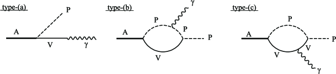
Figure 1: Feynman diagrams needed in the evaluation of the radiative axial-vector meson (A) decay.

In ref. [12] it was shown that, by invoking gauge invariance, only these diagrams need to be evaluated. In the next paragraph we elaborate further on this point. Let us look at the loop diagrams of fig. 1. Keeping in mind the dynamical origin of the resonance from the Bethe-Salpeter resummation of loops containing the kernel of the $VP\to VP$ interaction, the series implicit in those loops is given in fig. 2, where we have also added the second raw of diagrams to be discussed later on.

Figure 2: Series implicit in the type-b loop of fig. 1 in the dynamically generated picture of the axial-vector resonances

The photon coupled to the vector in the loop should be understood in the discussion, but is omitted to save diagrams. The requirement of gauge invariance would demand that the photon couples to all lines in the loops and vertices. This has been done in several works [22, 23, 24] dealing with photonuclear processes which involve dynamically generated resonances. An explicit proof of gauge invariance of this kind of diagrams can be seen in [23]. Thus, in addition to the diagrams of fig. 2 we would have diagrams like those in fig. 3.

Figure 3: Extra allowed diagrams required by gauge invariance.

Note that the $VP\to VP$ vertex is of the type $\epsilon_{V}\cdot\epsilon_{V}^{\prime}$ [14], with $\epsilon_{V}$ and $\epsilon_{V}^{\prime}$ the polarization vectors of the vector mesons, and thus has not photon contact term associated of the type $VVPP\gamma$. Diagrams $a)$ and $b)$ of fig. 3 are proportional to the last loop function with intermediate $P$ and $V$, which has the structure $J(Q^{2})Q^{\mu}$, with $Q$ the momentum of the produced pseudoscalar. However, as shown in the appendix of [12], this loop function satisfies $J(Q^{2}=m_{P}^{2})=0$, where $m_{P}$ is the mass of the produced pseudoscalar in the decay (see also ref. [25] for an alternative derivation with standard vector mesons, not dynamically generated). This is due to the requirement that the longitudinal part of the axial-vector propagator must not develop a pole of the pseudoscalar [26]. Radiation from the final pseudoscalar (see fig. 5) also leads to a null contribution, as discussed later. Thus, we are left with the diagrams of fig. 2 where the photon couples to the last loop, from where the pseudoscalar is emitted. The sum of loops before the last one generates the $VP$ T-matrix that contains the pole for the axial-vector [14]. The sum of diagrams is thus equivalent to the diagrams of fig. 4.

Figure 4: Equivalent representation of fig. 2 close to the axial-vector meson pole position.

The sum of diagrams of fig. 2 lead to a $VP\to\gamma P$ amplitude, in a simplified way omitting polarization vectors for simplicity,

$$-it=-it_{VP\to VP}L$$ (1)

where $L$ stands for the last loop function. Since $t_{VP\to VP}$ contains the axial-vector pole, close to the pole position, $s_{p}\simeq M_{A}^{2}-iM_{A}\Gamma$, we have

$$-it_{VP\to VP}=-i\frac{g_{AVP}^{2}}{s-s_{P}}.$$ (2)

Alternatively, from fig. 4 we would have

$$-it_{VP\to P\gamma}=-ig_{AVP}\frac{i}{s-s_{P}}(-i)g_{AP\gamma},$$ (3)

from where

$$g_{AP\gamma}=g_{AVP}L,$$ (4)

which is what we would directly obtain from the evaluations of diagrams of fig. 1 and what is done in [12], and which is the formalism followed in the present paper. The former slightly simplified derivation can be followed with more detail in [10] in the study of the radiative decay of the $\Lambda(1520)$ resonance. Once the equivalence of these formalisms is established, we can go back and reconsider the terms that one would have, which are shown in fig. 5,

Figure 5: Set of diagrams needed a priori in the evaluation of the axial-vector meson radiative decays.

the last two diagrams contributing in principle for charged axial-vector states. An explicit proof of the gauge invariance and finiteness of the set of diagrams of fig. 5, for the analogous case of $P\to V\gamma$ in the charm sector, is provided in [27]. Furthermore, in the appendix of [12] and [25] it is shown that diagram $e)$ of fig. 5 vanishes due to the Lorenz condition of the axial-vector meson ($\epsilon_{A}\cdot P_{A}=0$) (also noted in [27]) and diagram $d)$ of fig. 5 vanishes due to the condition $J(Q^{2}=m_{P}^{2})=0$, required to avoid a pole of the pseudoscalar in the longitudinal part of the axial-vector propagator [26], as stated above when discussing fig. 3.

After the above discussion we briefly recall the procedure followed in [12] to evaluate the radiative width, making explicit use of gauge invariance which simplifies considerably the calculation. Since the only external momenta available are $P$ (the axial-vector meson momentum) and $k$ (the photon momentum), the general expression of the amplitude can be written as

$$T={\epsilon_{A}}_{\mu}\epsilon_{\nu}T^{\mu\nu}$$ (5)

with

$$T^{\mu\nu}=a\,g^{\mu\nu}+b\,P^{\mu}P^{\nu}+c\,P^{\mu}k^{\nu}+d\,k^{\mu}P^{\nu}+e\,k^{\mu}k^{\nu}$$ (6)

In Eq. (5), $\epsilon_{A}$ and $\epsilon$ are the axial-vector meson and photon polarization vectors respectively. Note that, due to the Lorentz condition, ${\epsilon_{A}}_{\mu}P^{\mu}=0$, ${\epsilon}_{\nu}k^{\nu}=0$, all the terms in Eq. (5) vanish except for the $a$ and $d$ terms. On the other hand, gauge invariance implies that $T^{\mu\nu}k_{\nu}=0$, from where one gets

$$a=-d\,P\cdot k.$$ (7)

This is obviously valid in any reference frame, however, in the axial-vector meson rest frame and taking the Coulomb gauge for the photon, only the $a$ term survives in Eq. (5) since $\vec{P}=0$ and $\epsilon^{0}=0$. This means that, in the end, we will only need the $a$ coefficient for the evaluation of the process. However, the $a$ coefficient can be evaluated from the $d$ term thanks to Eq. (7). The advantage to evaluate only the $d$ coefficient is that the contact term of fig. 5c) does not contribute to the $d$ coefficient, only the loop diagrams of fig. 1 contribute, and from dimensional reasons (performing explicitly the Feynman integrals) one can see that the $d$ coefficients are finite for the diagrams of type-b in fig. 1. For the type-c diagrams, as discussed in [12] (after Eq. (25)), there was formally a logarithmic divergence coming from the $1/M_{V}^{2}$ term of the vector meson propagator, which required some tadpole from higher order terms for cancellation (see also ref. [28] in the analogous problem of $e^{+}e^{-}\to\phi f_{0}(980)$). In order to evaluate it we must use some regularization procedure. The most appropriate way to regularize the $1/M_{V}^{2}$ terms is to connect the divergences with those appearing in the basic problem of $VP\to VP$ scattering [14]. These divergencies already appear in the loop containing one pseudoscalar and one vector meson, which was regularized in [14] making use of the N/D method of [30] and dispersion relations. These allowed one to factorize on shell terms appearing in the numerator of the loop functions like the $q^{2}/M_{V}^{2}$ terms, with $q$ the vector meson momentum of the $VP$ loop [14]. In the present case one can estimate the contribution of the $q^{2}/M_{V}^{2}$ or the type-c loop by realizing that if one looks for sources of imaginary part by cutting diagram c) of fig. 1 by vertical lines, the cut to the left of the photon line can place two mesons on shell, for instance $\pi$ and $\rho$ for the $a_{1}$ resonance. The cut to the right of the photon, which would correspond to the energetically forbidden $\pi\to\pi\rho$ decay, does not provide imaginary part. Thus, the only source of the imaginary part comes from the cut at the left of the photon line, which is the same as that for the basic pseudoscalar-vector meson loop of the scattering problem. This allows us to replace momentum factors appearing in the numerator of the loop function, i.e. factors $q^{2}/M_{V}^{2}$, by its on shell value. The substitution is done in [14] after the $q^{0}$ integration is performed and one replaces $q^{2}/M_{V}^{2}$ by $\vec{q}\,^{2}_{\textrm{on}}/M_{V}^{2}$. Hence, the effects here are also of the order of $\vec{q}\,^{2}_{\textrm{on}}/M_{V}^{2}$ (there was an extra factor 1/3 for symmetry reasons in [14], which we ignore here to give a conservative estimate of the effects). Hence, we have checked that, for the most relevant cases, the estimate gives an upper limit of the order of 20% of the rest of the c) diagram. This value is of the same size as the finite results found in the diagrams of type-b, where the effect of the $1/M_{V}^{2}$ terms was of the order of $10\%$ or less. In the final results we will add in quadrature to the theoretical uncertainty a very conservative 10% of the total radiative decay width from this neglect of the $1/M_{V}^{2}$ terms in the type-c loops.

The Lagrangians needed in the evaluation of the diagrams in fig. 1 are given in ref. [12]. From these Lagrangians the tree level amplitude, type-a in fig. 1, takes the form

$$t_{a}=-g^{\prime}_{AVP}e\lambda_{V}F_{V}\frac{1}{M_{V}}\epsilon_{A}\cdot\epsilon$$ (8)

with $\lambda_{V}=1$, $1/3$, $-\sqrt{2}/3$ for $\rho$, $\omega$ and $\phi$ respectively, $F_{V}=156\pm 5$MeV [29], $M_{V}$ is the vector meson mass and $e$ is taken positive. In Eq. (8), $g^{\prime}_{AVP}$ is the $AVP$ coupling in the charge base. These coefficients are related to the $g_{AVP}$ in isospin base, obtained in ref. [14], through the transformation

$$g^{\prime}_{AVP}={\cal C}\times g_{AVP},$$ (9)

where ${\cal C}$ are coefficients dependent on the different $AVP$ channels summarized in tables 1–6. In the present work we use the values of $g_{AVP}$ obtained in refs. [14, 12] by evaluating the residua at the pole position of the different $VP\to VP$ scattering amplitudes.

$h_{1}(1170/1380)\rightarrow\pi^{0}\gamma$		${\cal C}$	$Q$	$c_{VPP}$
tree	$\rho$	$-1/\sqrt{3}$	-	-
type-b	$\rho^{-}\pi^{+}$	$-1/\sqrt{3}$	$e$	$\sqrt{2}$
	$\rho^{+}\pi^{-}$	$-1/\sqrt{3}$	$-e$	$-\sqrt{2}$
	${K^{*}}^{-}K^{+}$	1/2	$e$	$1/\sqrt{2}$
	${K^{*}}^{+}K^{-}$	1/2	$-e$	$-1/\sqrt{2}$
type-c	$\rho^{-}\pi^{+}$	$-1/\sqrt{3}$	$-e$	$\sqrt{2}$
	$\rho^{+}\pi^{-}$	$-1/\sqrt{3}$	$e$	$-\sqrt{2}$
	${K^{*}}^{-}K^{+}$	1/2	$-e$	$1/\sqrt{2}$
	${K^{*}}^{+}K^{-}$	1/2	$e$	$-1/\sqrt{2}$

Table 1: Coefficients in eqs. (8), (9), (10) and (11) for $h_{1}(1170/1380)\rightarrow\pi^{0}\gamma$ decay.

$h_{1}(1170/1380)\rightarrow\eta\gamma$		${\cal C}$	$Q$	$c_{VPP}$
tree	$\phi$	1	-	-
	$\omega$	1	-	-
type-b	${K^{*}}^{-}K^{+}$	1/2	$e$	$\sqrt{3/2}$
	${K^{*}}^{+}K^{-}$	1/2	$-e$	$-\sqrt{3/2}$
type-c	${K^{*}}^{-}K^{+}$	1/2	$-e$	$\sqrt{3/2}$
	${K^{*}}^{+}K^{-}$	1/2	$e$	$-\sqrt{3/2}$

Table 2: Coefficients in eqs. (8), (9), (10) and (11) for $h_{1}(1170/1380)\rightarrow\eta\gamma$ decay.

$b_{1}^{0}(1235)\rightarrow\pi^{0}\gamma$		${\cal C}$	$Q$	$c_{VPP}$
tree	$\phi$	1	-	-
	$\omega$	1	-	-
type-b	${K^{*}}^{-}K^{+}$	$-1/2$	$e$	$1/\sqrt{2}$
	${K^{*}}^{+}K^{-}$	$-1/2$	$-e$	$-1/\sqrt{2}$
type-c	${K^{*}}^{-}K^{+}$	$-1/2$	$-e$	$1/\sqrt{2}$
	${K^{*}}^{+}K^{-}$	$-1/2$	$e$	$-1/\sqrt{2}$

Table 3: The coefficients for $b_{1}^{0}(1235)\rightarrow\pi^{0}\gamma$ decay.

$b_{1}^{0}(1235)\rightarrow\eta\gamma$		${\cal C}$	$Q$	$c_{VPP}$
tree	$\rho$	1	-	-
type-b	${K^{*}}^{-}K^{+}$	$-1/2$	$e$	$\sqrt{3/2}$
	${K^{*}}^{+}K^{-}$	$-1/2$	$-e$	$-\sqrt{3/2}$
type-c	${K^{*}}^{-}K^{+}$	$-1/2$	$-e$	$\sqrt{3/2}$
	${K^{*}}^{+}K^{-}$	$-1/2$	$e$	$-\sqrt{3/2}$

Table 4: The coefficients for $b_{1}^{0}(1235)\rightarrow\eta\gamma$ decay.

$K_{1}^{+}(1270)\rightarrow K^{+}\gamma$		${\cal C}$	$Q$	$c_{VPP}$
tree	$\phi$	1	-	-
	$\omega$	1	-	-
	$\rho$	$-1/\sqrt{3}$	-	-
type-b	$\phi K^{+}$	1	$e$	1
	$\omega K^{+}$	1	$e$	$-1/\sqrt{2}$
	$\rho^{0}K^{+}$	$-1/\sqrt{3}$	$e$	$-1/\sqrt{2}$
	${K^{*}}^{0}\pi^{+}$	$\sqrt{2/3}$	$e$	1
type-c	$\rho^{+}K^{0}$	$-\sqrt{2/3}$	$e$	$-1$
	${K^{*}}^{+}\eta$	1	$e$	$\sqrt{3/2}$
	${K^{*}}^{+}\pi^{0}$	$1/\sqrt{3}$	$e$	$1/\sqrt{2}$

Table 5: The coefficients in eqs.(8), (10) and (11) for ${K_{1}}^{+}\rightarrow K^{+}\gamma$ decay.

$K_{1}^{0}(1270)\rightarrow K^{0}\gamma$		${\cal C}$	$Q$	$c_{VPP}$
tree	$\phi$	1	-	-
	$\omega$	1	-	-
	$\rho$	$1/\sqrt{3}$	-	-
type-b	$\rho^{-}K^{+}$	$-\sqrt{2/3}$	$e$	$-1$
	${K^{*}}^{+}\pi^{-}$	$\sqrt{2/3}$	$-e$	1
type-c	$\rho^{-}K^{+}$	$-\sqrt{2/3}$	$-e$	$-1$
	${K^{*}}^{+}\pi^{-}$	$\sqrt{2/3}$	$e$	1

Table 6: The coefficients in eqs.(8), (10) and (11) for ${K_{1}}^{0}\rightarrow K^{0}\gamma$ decay.

Eq. (8) is formally not gauge invariant. An alternative derivation using tensor formalism is given in ref. [9] and replaces $\epsilon_{A}\cdot\epsilon$ by $(\epsilon_{A}\cdot\epsilon-\epsilon_{A}\cdot k\,\epsilon\cdot P/k\cdot P)$ with $P$ and $k$ the axial-vector meson and photon momenta respectively. Then the amplitude becomes manifestly gauge invariant and reduces to Eq. (8) in the Coulomb gauge ($\epsilon^{0}=0$) which we use to evaluate the amplitudes.

In ref. [12], the contribution to the total amplitude from type-b loops is shown to be convergent by invoking gauge invariance. This amplitude is given by

$$t_{\rm b} = -g^{\prime}_{AVP}Qc_{VPP}\frac{M_{V}G_{V}}{\sqrt{2}f^{2}}2P\cdot k\epsilon_{A}\cdot\epsilon$$ (10)

$$\times \int_{0}^{1}dx\int_{0}^{x}dy\frac{1}{32\pi^{2}}\frac{1}{s+i\varepsilon}\left\{-4(1-x)\left(1+\frac{y(xP-yk)\cdot(k-P)}{M_{V}^{2}}\right)\right\},$$

where $Q$ is the charge of the meson in the loop emitting the photon and $c_{VPP}$ are numerical coefficients coming from the $VPP$ Lagrangian [12] and are given in tables 1–6. In Eq. (10) $G_{V}$ is the $VPP$ coupling in the notation of [7] and for the numerical value we take $G_{V}=55\pm 5$ MeV from ref. [29], $f$ is the pion decay constant ($f=93\textrm{ MeV}$), $\epsilon_{A(\gamma)}$ is the axial-vector(photon) polarization vector. The coefficients shown in these tables for the channels with an $\eta$ meson in the final state are for the decay into $\eta_{8}$. Hence, in order to obtain the appropriate width of the channels decaying into $\eta\gamma$ we have to multiply the decay width for these channels by $8/9$, from the consideration of the mixing $\eta=\eta_{1}/3+2\sqrt{2}/3\eta_{8}$.

The amplitude from the type-c loop, neglecting the formally logarithmically divergent but very small $1/M_{V}^{2}$ terms [12], is given by:

$$t_{\rm c} = g^{\prime}_{AVP}Qc_{VPP}\frac{M_{V}G_{V}}{\sqrt{2}f^{2}}2P\cdot k\epsilon_{A}\cdot\epsilon$$ (11)

$$\times \int_{0}^{1}dx\int_{0}^{x}dy\frac{1}{32\pi^{2}}\frac{1}{s^{\prime}+i\varepsilon}(1-3x+2y+y(1-x)).$$

With these amplitudes, the decay width for the axial-vector mesons into one pseudoscalar meson and one photon is given by

$$\Gamma(M_{A})=\frac{|\vec{k}|}{12\pi M_{A}^{2}}|T|^{2},$$ (12)

where $M_{A}$ stands for the mass of the decaying axial-vector meson and $T$ is the sum of the amplitudes from the tree level and loop mechanisms removing the $\epsilon_{A}\cdot\epsilon$ factor. The former expression is valid in the limit of narrow axial-vector resonance. In order to take into account the finite width of the axial-vector meson we fold the previous expression with the mass distribution:

$$\Gamma_{A\rightarrow P\gamma}=-\frac{1}{\pi}\int_{(M_{A}-2\Gamma_{A})^{2}}^{(M_{A}+2\Gamma_{A})^{2}}ds_{A}\,Im\left\{\frac{1}{s_{A}-M_{A}^{2}+iM_{A}\Gamma_{A}}\right\}\Gamma(\sqrt{s_{A}})\Theta(\sqrt{s_{A}}-\sqrt{s_{A}^{th}}),$$ (13)

where $\Theta$ is the step function, $\Gamma_{A}$ is the total axial-vector meson width and $s_{A}^{th}$ is the threshold for the dominant $A$ decay channels.

Similarly, since the $\rho$ and $K^{*}$ mesons have relatively large widths, we have also taken into account the mass distribution of these states in the loop functions leading to the $t_{b}$ and $t_{c}$ amplitudes. This is done by folding $t_{b}$, $t_{c}$, with the spectral function of the $\rho$ and $K^{*}$:

$$t_{b,c}\to t_{b,c}=-\frac{1}{\pi}\int_{(M_{V}-2\Gamma_{V})^{2}}^{(M_{V}+2\Gamma_{V})^{2}}ds_{V}\,Im\left\{\frac{1}{s_{V}-M_{V}^{2}+iM_{V}\Gamma_{V}}\right\}t_{b,c}(\sqrt{s_{V}}).$$ (14)

The corrections from this source are small, they change the radiative widths at the level of $2$% or below, although the contribution of some intermediate states, which are particularly suppressed, experiences larger changes.

3 Results for the different channels

In what follows we discuss in detail the results for the radiative decays of the different axial-vector resonances. We will refer to the results shown in tables 7–12 where we show the contributions of the different mechanisms to the radiative decay widths. The theoretical errors quoted have been obtained by doing a Monte-Carlo sampling of the parameters of the model within their uncertainties, as explained in ref. [12]. Note that in ref. [14] all the pole positions, and hence the couplings to the different channels, were obtained with the same value for the only free parameter of the model, the subtraction constant, of $a=-1.85$ (see reference [14] for details). But we can use different subtraction constants for different ($S$, $I$, $G$-parity) channels. Therefore, in order to get a more accurate result, we have fine tuned the subtraction constants such that the real part of the pole positions agrees better with the experimental axial-vector masses. On the other hand, one can also assign an uncertainty to the $f$ constant appearing in the Lagrangians since it could range from $f_{\pi}$ to $f_{\eta}$, averaging $1.15\times 92$ MeV. We have also considered this uncertainty in our calculations. The central values in the tables are obtained using $f=1.08\times f_{\pi}$ and the central values for the rest of the parameters (except for the $K_{1}$ case where the more refined values of ref. [20] for the couplings and a different central value for $f$ are used). On the other hand, an extra conservative $10$% has been added in quadrature to the error in order to consider the uncertainty from the neglect of the $1/M_{V}^{2}$ terms in the evaluation of the type-c loop contribution, as explained in the previous section.

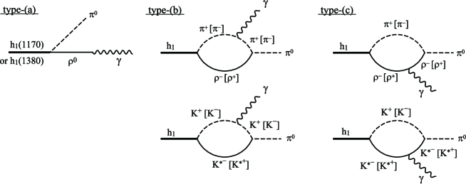
Figure 6: Feynman diagrams contributing to $h_{1}(1170)\rightarrow\pi^{0}\gamma$ decay and $h_{1}(1380)\rightarrow\pi^{0}\gamma$ decay.

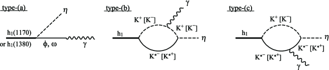
Figure 7: Feynman diagrams contributing to $h_{1}(1170)\rightarrow\eta\gamma$ decay and $h_{1}(1380)\rightarrow\eta\gamma$ decay.

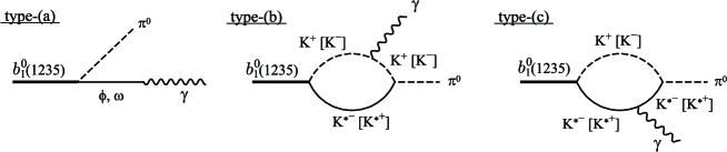
Figure 8: Feynman diagrams contributing to $b_{1}^{0}(1235)\rightarrow\pi^{0}\gamma$ decay.

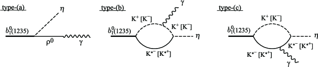
Figure 9: Feynman diagrams contributing to $b_{1}^{0}(1235)\rightarrow\eta\gamma$ decay.

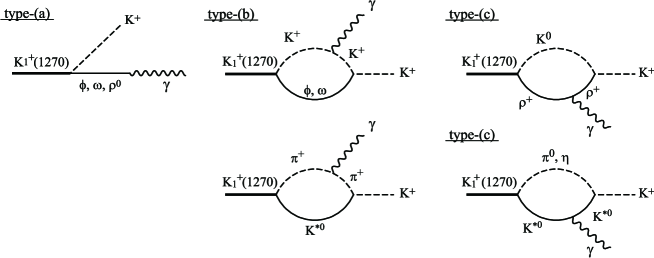
Figure 10: Feynman diagrams contributing to $K_{1}^{+}(1270)\rightarrow K^{+}\gamma$ decay.

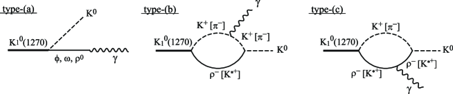
Figure 11: Feynman diagrams contributing to $K_{1}^{0}(1270)\rightarrow K^{0}\gamma$ decay.

		$h_{1}(1170)$	$h_{1}(1380)$
tree	$\rho$	294.8	9.1
	total	294.8	9.1
type-b	$\rho^{-}\pi^{+}$	51.8	2.2
	$\rho^{+}\pi^{-}$	same as $\rho^{-}\pi^{+}$
	${K^{*}}^{-}K^{+}$	0.43	15.2
	${K^{*}}^{+}K^{-}$	same as ${K^{*}}^{-}K^{+}$
	total	226.0	37.0
type-c	$\rho^{-}\pi^{+}$	0.30	$1.5\times 10^{-2}$
	$\rho^{+}\pi^{-}$	same as $\rho^{-}\pi^{+}$
	${K^{*}}^{-}K^{+}$	$2.2\times 10^{-3}$	$6.5\times 10^{-2}$
	${K^{*}}^{+}K^{-}$	same as ${K^{*}}^{-}K^{+}$
	total	1.34	0.51
	loop total	218.0	45.8
TOTAL		$837\pm 134$	$81\pm 18$

Table 7: $h_{1}(1170)$/$h_{1}(1380)\rightarrow\pi^{0}\gamma$ decay widths in units of keV.

		$h_{1}(1170)$	$h_{1}(1380)$
tree	$\phi$	$2.0\times 10^{-2}$	36.3
	$\omega$	$3.5\times 10^{-3}$	21.3
	total	$1.24\times 10^{-2}$	113.3
type-b	${K^{*}}^{-}K^{+}$	0.75	28.5
	${K^{*}}^{+}K^{-}$	same as ${K^{*}}^{-}K^{+}$
	total	3.01	113.9
type-c	${K^{*}}^{-}K^{+}$	$2.71\times 10^{-3}$	0.085
	${K^{*}}^{+}K^{-}$	same as ${K^{*}}^{-}K^{+}$
	total	$1.08\times 10^{-2}$	0.34
	loop total	3.37	126.6
TOTAL		$3.1\pm 0.9$	$438\pm 80$

Table 8: $h_{1}(1170)$/$h_{1}(1380)\rightarrow\eta\gamma$ decay widths in units of keV.

		$b_{1}^{0}(1235)$
tree	$\phi$	19.7
	$\omega$	14.1
	total	66.9
type-b	${K^{*}}^{-}K^{+}$	6.6
	${K^{*}}^{+}K^{-}$	same as ${K^{*}}^{-}K^{+}$
	total	26.3
type-c	${K^{*}}^{-}K^{+}$	$3.3\times 10^{-2}$
	${K^{*}}^{+}K^{-}$	same as ${K^{*}}^{-}K^{+}$
	total	0.13
	loop total	30.1
TOTAL		$180\pm 28$

Table 9: $b_{1}^{0}(1235)\rightarrow\pi^{0}\gamma$ decay width in units of keV.

		$b_{1}^{0}(1235)$
tree	$\rho$	244.0
	total	244.0
type-b	${K^{*}}^{-}K^{+}$	10.8
	${K^{*}}^{+}K^{-}$	same as ${K^{*}}^{-}K^{+}$
	total	43.2
type-c	${K^{*}}^{-}K^{+}$	$3.8\times 10^{-2}$
	${K^{*}}^{+}K^{-}$	same as ${K^{*}}^{-}K^{+}$
	total	0.15
	loop total	48.5
TOTAL		$488\pm 70$

Table 10: $b_{1}^{0}(1235)\rightarrow\eta\gamma$ decay width in units of keV.

		$K_{1}(1270)$
		pole-A	pole-B
		$1195-123i$	$1284-73i$
tree	$\phi$	24.7	8.3
	$\omega$	17.4	5.3
	$\rho^{0}$	58.4	253.8
	total	8.58	412.5
type-b	$\phi K^{+}$	2.4	0.80
	$\omega K^{+}$	3.3	1.0
	$\rho^{0}K^{+}$	0.9	3.9
	${K^{*}}^{0}\pi^{+}$	41.9	2.7
	total	68.4	25.7
type-c	$\rho^{+}K^{0}$	$3.0\times 10^{-2}$	0.13
	${K^{*}}^{+}\eta$	$2.3\times 10^{-4}$	$6.4\times 10^{-2}$
	${K^{*}}^{+}\pi^{0}$	0.12	$7.5\times 10^{-3}$
	total	0.15	0.26
	loop total	75.3	20.9
TOTAL		$34\pm 13$	$251\pm 56$

Table 11: $K_{1}^{+}(1270)\rightarrow K^{+}\gamma$ widths for two poles in units of keV.

		$K_{1}(1270)$
		pole-A	pole-B
		$1195-123i$	$1284-73i$
tree	$\phi$	24.7	8.3
	$\omega$	17.4	5.3
	$\rho_{0}$	58.4	253.8
	total	274.3	148.7
type-b	$\rho^{-}K^{+}$	3.6	15.5
	${K^{*}}^{+}\pi^{-}$	41.8	2.7
	total	61.5	6.7
type-c	$\rho^{-}K^{+}$	$3.0\times 10^{-2}$	0.13
	${K^{*}}^{+}\pi^{-}$	0.47	$3.0\times 10^{-2}$
	total	0.48	0.28
	loop total	57.6	9.7
TOTAL		$512\pm 73$	$227\pm 79$

Table 12: $K_{1}^{0}(1270)\rightarrow K^{0}\gamma$ widths for two poles in units of keV.

3.1 $S=0$, $I=0$ channel

$h_{1}(1170)$/$h_{1}(1380)\rightarrow\pi^{0}\gamma$

The $S=0$, $I=0$ and negative $G$-parity axial-vector mesons couple to $\phi\eta$, $\omega\eta$, $\rho\pi$ and the combination $1/\sqrt{2}(\bar{K^{*}}K-K^{*}\bar{K})$ in our model. However, the first two channels lead to b and c type diagrams with neutral intermediate mesons and do not contribute. Hence, only the diagrams shown in fig. 6, with $\rho\pi$ and $K^{*}K$ in the loops, contribute to the process. For the tree level diagram only the $\rho$ meson exchange is possible. In our model, the $h_{1}(1170)$ resonance has a coupling to the $\rho\pi$ channel that is about five times the one of $h_{1}(1380)$. Altogether this makes the tree level and the $\rho\pi$ loop contributions much larger for the $h_{1}(1170)$ decay than for the $h_{1}(1380)$ one, as seen in table 7. This implies at the end, after the coherent sum of all the contributions, that the radiative decay width of the $h_{1}(1170)$ into $\pi\gamma$ is much larger than that of the $h_{1}(1380)$ and, hopefully, it could be measured experimentally given its large value $863\pm 134$ keV. Note the important role of the loop contribution which makes that the final result obtained for the $h_{1}(1170)$ is about a factor $3$ larger than considering only the tree level mechanism and about a factor $9$ for the $h_{1}(1380)$ case.

$h_{1}(1170)$/$h_{1}(1380)\rightarrow\eta\gamma$

The diagrams needed in the evaluation of this process are shown in fig.7. The couplings of the $h_{1}(1170)$ to the $\omega\eta$ and $\phi\eta$ channels are very small. This makes the tree level almost negligible. This is not the case for the $h_{1}(1380)$ resonance since its couplings to these channels are much larger. On the other hand, the loop contributions are also smaller for the $h_{1}(1170)$ since its coupling to $1/\sqrt{2}(\bar{K^{*}}K-K^{*}\bar{K})$ is about a factor four smaller than that of the $h_{1}(1380)$ resonance. All these facts, together with the constructive interference between the loops and the tree level in the $h_{1}(1380)$ case, make the radiative decay width of the $h_{1}(1380)$ two orders of magnitude larger than the $h_{1}(1170)$.

$f_{1}(1285)\rightarrow\pi^{0}\gamma$

This channel is zero by ${\cal C}$-parity conservation.

3.2 $S=0$, $I=1$ channel

The radiative decays into $\pi\gamma$ of the charged $a_{1}(1260)$ and $b_{1}(1235)$ resonances were thoroughly discussed in ref. [12], and hence we only consider in the present paper the neutral $S=0$, $I=1$, axial-vector radiative decay modes.

$a_{1}^{0}(1260)\rightarrow\pi^{0}\gamma$

This channel is zero by ${\cal C}$-parity conservation. However, as seen in ref. [12], the charged decay channel, $a_{1}^{\pm}(1260)\rightarrow\pi^{\pm}\gamma$, was allowed and had a large decay width.

$b_{1}^{0}(1235)\rightarrow\pi^{0}\gamma$

The $b_{1}(1235)$ couples to the positive $G$-parity $VP$ states $1/\sqrt{2}(\bar{K^{*}}K+K^{*}\bar{K})$, $\phi\pi$, $\omega\pi$ and $\rho\eta$. The allowed Feynman diagrams are shown in fig. 8. One can see from table 9 that the tree level only accounts for $\sim 1/3$ of the final result. This illustrates the important role of the loops considered in the present formalism. It is worth stressing that the result obtained for the $b_{1}^{0}(1235)\rightarrow\pi^{0}\gamma$ decay is the same as for the $b_{1}^{\pm}(1235)\rightarrow\pi^{\pm}\gamma$ decay obtained in [12], unlike the $a_{1}(1260)$ case, as explained above.

$b_{1}^{0}(1235)\rightarrow\eta\gamma$

The allowed Feynman diagrams are shown in fig. 9. As can be seen in table 10, the tree level contribution to the decay width for this channel is much larger than in the $b_{1}^{0}(1235)\rightarrow\pi^{0}\gamma$ (despite the phase space available) since the coupling to $\rho\eta$ is larger than to $\omega\pi$ and $\phi\pi$. This size of the tree level, together with the constructive interference with the loop contributions, makes the final radiative width for this channel very large, about a factor $\sim 3$ larger than the $b_{1}^{0}(1235)\rightarrow\pi^{0}\gamma$ decay rate.

3.3 Consideration of higher mass intermediate states

In principle we could consider in our approach the contribution of additional channels involving vector-pseudoscalar states of higher masses. The contributions of such channels in the chiral unitary approach leading to the axial-vector mesons [14] was omitted, as usually done in this approach. The idea is that they, being far off shell in the loops, provide a small contribution, but more important, they can be reabsorbed into the subtraction constant of the dispersion relation which provides the loop function, because their contribution is very weakly energy dependent. In the present work, where the loops are finite, the contribution from these channels would be additive. We make here an estimation of the contribution of these heavy states.

The first consideration is that when one has many channels in the chiral unitary approach, the coupling of the resonance to the channels with mass far from the resonance mass is very weak as a general rule. For instance, the coupling of the $\sigma(600)$ to $\eta\eta$ is about $4$% of the one to $\pi\pi$ [30]. The coupling of the $\Lambda(1405)$ to $K\Xi$ is of the order of one fourth of the dominant $\pi\Sigma$ and $\bar{K}N$ channels. We should keep this fact in mind. To make the estimates of the high mass states contribution in the present case, we take intermediate states where the $\pi$ is replaced by the $\pi(1300)$ and other states where the $\rho$ is substituted by the $\rho(1450)$, the next pseudoscalar and vector excited states. We assume first the loops changing $\pi$ to $\pi(1300)$. We take in a first run the couplings in the loop the same as for $\pi$ and investigate only the effect of the change in the mass. We get contributions of the order of $2$% of the contribution of the loops of $\rho\pi$ in the $h_{1}$ decays and in the $K^{*}\pi$ of the $K_{1}$ decay from the type-b loops. In type-c loops, for some intermediate states the relative contribution of the $\pi(1300)$ with respect to the $\pi$ case is larger but these terms have very small weight. Next we should consider the difference between the $\rho\pi\pi$ and $\rho\pi\pi(1300)$ couplings. By looking at $\rho\to\pi\pi$ and $\pi(1300)\to\rho\pi$ decays, assuming $\Gamma(1300)\sim 400\textrm{ MeV}$ from the PDG [31] and all strength of $\pi(1300)$ going to $\rho\pi$, we obtain a ratio of couplings $g_{\pi\pi^{\prime}\rho}/g_{\pi\pi\rho}=1.8$, which should be compensated from the smaller coupling of the axial-vector resonances to the $\rho\pi(1300)$ state. The effect at the end in the total radiative width of the resonance is smaller than the one quoted above from some particular channels and is far smaller than the uncertainties in the results from the other sources considered here.

Next we do the same exercise by changing the $\rho$ to the $\rho(1450)$. The change of the mass without changing coupling constants is in general very small with the exception of the contribution of the intermediate state $\rho(1450)\pi$ for the two $h_{1}$ decays. In this case the contribution of the new loop to $t_{b}$ is $17$% of the contribution of the $\rho(770)\pi$. However, we should now take into account the ratio $g_{\rho(1450)\pi\pi}/g_{\rho\pi\pi}=0.5$ following the same steps as before, assuming in the worse of the cases that all the $\rho(1450)$ width comes from $\pi\pi$. This changes in a maximum of $8$% the contributions to $t_{b}$ from this intermediate state. With a conservative estimate of a factor of two reduction from the coupling of the axial-vector resonance to this new channel, this results in a $4$% change of the contribution to $t_{b}$ from the $\rho\pi$ channel. When this new contribution is added to all other terms it has a repercussion of a maximum $4$% change in the total decay rate for the $h_{1}(1170)$ and much smaller for the $h_{1}(1380)$. Once again this uncertainty is smaller than the one obtained before from other sources.

4 Consequences of the two $K_{1}(1270)$ poles

We have singled out the $S=1$, $I=1/2$, sector into this different section since it deserves particular attention for the following reasons. In the first place, in the work of ref. [14], two poles were found in the $S=1$, $I=1/2$, $VP$ scattering amplitude which were assigned there to two $K_{1}(1270)$ resonances instead of the usual $K_{1}(1270)$ and $K_{1}(1400)$. In table 13 we show the two pole positions and the couplings to the different $VP$ channels of the two $K_{1}(1270)$ resonances obtained in [20]. In the following, we call pole-A the lowest mass pole and pole-B the highest mass one. Some possible experimental consequences of this double pole structure of the $K_{1}(1270)$ resonance were already discussed in ref. [20]. If this double pole reflects the real nature of these resonance, it would have significant relevance in the study of the radiative decays both from the theoretical and experimental points of view. Indeed, there is experimental information [21] on the decay width of the process $K_{1}^{0}(1270)\rightarrow K^{0}\gamma$ which relies in an experimental analysis that does not consider the two pole structure. The result for the radiative width would change had the two pole nature of the $K_{1}(1270)$ been considered, as we will discuss in this section.

First of all let us present our theoretical results for the radiative decay widths of $K_{1}^{\pm}$ and $K^{0}$ for both poles A and B.

$K_{1}^{+}(1270)\rightarrow K^{+}\gamma$

The possible intermediate channels in the tree level and type-b and -c loops for the $K^{+}_{1}(1270)$ radiative decay are shown in fig. 10. The results for the different contributions for both poles A and B are shown in table 11. In this table one can see that the tree level contribution for the pole-B is about a factor fifty larger than for the pole-A. This is due to the fact that the coupling of the pole-B to the $\rho K$ channel is about a factor two larger than for the pole-A (see table 13) and to the different sign of the $\rho K$ couplings for both poles (see table 13), what makes the interference with the $\phi$ and $\omega$ contributions different. The difference in the couplings to the $VP$ channels for the pole-A and B, both in sign and absolute value, is also responsible for the different value of the loop contributions and the sign of the interference, leading to a final result for the radiative width which is about an order of magnitude larger for the B-pole.

$K_{1}^{0}(1270)\rightarrow K^{0}\gamma$

For the $K_{1}^{0}(1270)$ radiative decay, the allowed mechanisms are shown in fig. 11. Note the different allowed particles in the loops with respect the $K_{1}^{+}(1270)$ case (fig. 10), like for instance the presence of $\rho$ instead of $\phi$ and $\omega$ in the type-b loop.

Unlike the $K_{1}^{+}(1270)$ case, we obtain similar values of the tree level contributions for both poles, while the individual contributions to the tree level are the same as in the $K_{1}^{+}$ case (see tables 11 and 12). This is due to the different sign of $K_{1}^{0}$ to the $\rho K$ channel in the charge base from that of $K_{1}^{+}$, as can be seen in tables 5 and 6. Note that the ${K^{*}}\pi$ loop contribution for the pole-A is larger than the $\rho K$, while for the pole-B the $\rho K$ contribution is larger than $K^{*}\pi$. This is a consequence of the fact that the largest coupling for the pole-A is to ${K^{*}}\pi$ while for the pole-B is to the $\rho K$ channel.

4.1 Discussion on the experimental result

Unlike the other channels, there is experimental information about the $K_{1}^{0}(1270)\rightarrow K^{0}\gamma$ decay width. This radiative decay width has already been measured at Fermilab [21]. In the analysis of this experiment [21] it was concluded that the radiative decay width of $K_{1}(1270)$ is $73.2\pm 6.1({\rm stat})\pm 8.2({\rm int\ syst})\pm 27.0({\rm ext\ syst})$ keV and that of $K_{1}(1400)$ is $280.8\pm 23.2({\rm stat})\pm 31.4({\rm int\ stat})\pm 25.4({\rm ext\ stat})$ keV. This is in remarkable disagreement with our results mentioned above and in table 12. However this discrepancy can be explained in view of the two pole structure of the $K_{1}(1270)$ resonance, not considered in the experimental analysis:

The experiment [21] did not measure the $K_{1}(1270)$ radiative decay directly. Since direct observation of radiative decays such as $K_{1}\rightarrow K+\gamma$ is difficult, they measured the $K_{1}$ radiative decay using the inverse reaction $K+\gamma\rightarrow K_{1}$, which can be performed experimentally using the $K+{\rm nucleus}\rightarrow K_{1}+{\rm nucleus}$ reaction with Primakoff effect [32]. The experiment obtained 147 events for strange axial-vector mesons reconstructed from $K^{*}\pi$ final state and used them to estimate the radiative widths for $K_{1}(1270)$ and $K_{1}(1400)$. But in the experimental analysis it is assumed that there is only one $K_{1}(1270)$ and a $K_{1}(1400)$ resonances contributing to the events. The traditional approach to the $K_{1}(1270)$ and $K_{1}(1400)$ resonances, and the one assumed in the experiment, is that they are a mixture of a singlet and triplet component

$$K_{1}(1400) = {}^{3}P_{1}\cos\theta+^{1}P_{1}\sin\theta$$ (15)

$$K_{1}(1270) = -^{3}P_{1}\sin\theta+^{1}P_{1}\cos\theta.$$ (16)

The value for the mixing angle used in the experimental analysis [21] is $\theta=56^{\circ}\pm 3^{\circ}$ [33] but there is controversy about this value (see the discussion in the introduction of ref. [9]) and very different mixing angles are quoted from the study of $J/\Psi$ decay [34]. As quoted in [20] this could be a problem related to the existence of two $K_{1}(1270)$ resonances. Coming back to the experimental analysis of ref. [21], since the triplet component is not excited by the Coulomb field [35], the $K_{1}$ production rates would be proportional to $\cos^{2}\theta$ for the $K_{1}(1400)$ and $\sin^{2}\theta$ for the $K_{1}(1270)$ from where the ratio of $72.2$ keV for the $K_{1}(1270)$ and $280.8$ keV for the $K_{1}(1400)$ was deduced in the experimental analysis. However, in our approach this mixing scheme would be different since the mixing would be between two $K_{1}(1270)$ resonances, and possibly a $K_{1}(1400)$, rather than between only one $K_{1}(1270)$ and a $K_{1}(1400)$. If there are actually two $K_{1}(1270)$ poles, instead of just one, this invalidates the different weights assigned to the $K_{1}(1270)$ and the $K_{1}(1400)$ in ref. [21].

Let us hence make an alternative guess. The experiment[21] observed the ${K^{*}}^{0}(892)\pi^{0}$ channel in the final state, hence as a subprocess of the experimental reaction we have the mechanisms shown in fig. 12.

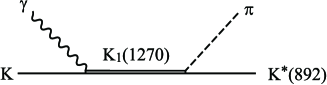
Figure 12: Subprocess in the experimental mechanism producing the $K_{1}$ with $K^{*}\pi$ in the final state.

In our model, we have two poles for the $K_{1}(1270)$ resonance. In this case, the contributions of these two poles should interfere. We can estimate the effect of this interference in the experiment as follows. The amplitude of the subreaction process in the experiment, shown in fig. 12, for the two different poles can be written approximately as

$$T_{A} = g_{{K^{*}}^{0}\pi^{0}}^{A}g_{K^{0}\gamma}^{A}\frac{1}{{s_{K_{1}}-M^{A}_{K_{1}}}^{2}+iM^{A}_{K_{1}}\Gamma^{A}_{K_{1}}},$$

$$T_{B} = g_{{K^{*}}^{0}\pi^{0}}^{B}g_{K^{0}\gamma}^{B}\frac{1}{{s_{K_{1}}-M^{B}_{K_{1}}}^{2}+iM^{B}_{K_{1}}\Gamma^{B}_{K_{1}}},$$ (17)

where $g_{{K^{*}}^{0}\pi^{0}}^{A(B)}$ is the coupling of the $K_{1}^{0}(1270)$ pole-A(B) to ${K^{*}}^{0}\pi^{0}$ channel in charge base as

$$g_{{K^{*}}^{0}\pi^{0}}^{A(B)}=-\frac{1}{\sqrt{3}}g_{K^{*}\pi}^{A(B)}$$

with $g_{K^{*}\pi}^{A(B)}$ being the coupling of the pole-A(B) to $K^{*}\pi$ in isospin base. In Eq. (17) $g_{K^{0}\gamma}^{A(B)}$ is the coupling constant of the $K_{1}^{0}(1270)$ pole-A(B) to the $K^{0}\gamma$ which can be evaluated from the radiative decay amplitudes obtained in this paper at $\sqrt{s_{K_{1}}}=M_{K_{1}}$ if we define $t_{K_{1}^{0}\to K^{0}\gamma}=g_{K_{1}^{0}K^{0}\gamma}\epsilon_{A}\cdot\epsilon$. In Eq. (17) the masses and widths used in the propagators are the ones given by the poles of table 13. The couplings that we found for the different poles are shown in table 13.

	pole-A		pole-B
	$g^{A}$	$|g^{A}|$	$g^{B}$	$|g^{B}|$
$K^{0}\gamma$	$217-96i$	$237$	$-166-66i$	$179$
${K^{*}}^{0}\pi^{0}$	$-2740+1659i$	$3203$	$-444+676i$	$809$
$\rho^{0}K^{0}$	$-965+923i$	$1335$	$2774+228i$	$2783$

Table 13: The coupling constants of the two $K_{1}^{0}(1270)$ to $K^{0}\gamma$, ${K^{*}}^{0}\pi^{0}$ and $\rho^{0}K^{0}$ in charge base.

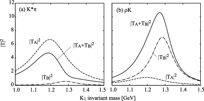
Figure 13: The squared amplitudes corresponding eqs. (17) and their coherent sums for (a) $K^{*}\pi$ and (b) $\rho K$ in final states, as functions of the $K_{1}$ invariant mass.

As we can see from table 13, the coupling of the pole-A to the $K^{*}\pi$ channel is about four times larger than the pole-B. Hence, this process is dominated by the pole-A contribution. In fig. 13(a) we show the modulus squared of $T_{A}$, $T_{B}$, of Eq. (17) and the coherent addition of both amplitudes. Since the sign of the two $K_{1}$ couplings to $K\gamma$ are different for both poles, the interference between $T_{A}$ and $T_{B}$ is destructive for the $K^{*}\pi$ case. This means that the amplitude observed in such a experiment should be smaller than the one obtained with the dominant amplitude. The ratio $|T_{A}+T_{B}|^{2}/|T_{A}|^{2}$ is $\sim 0.7$, and hence the corresponding radiative decay width observed in such experiment from our model would be $525$ keV$\times 0.7=370$ keV. This value is much similar to the addition of the experimental values of the radiative decay width of the $K_{1}(1270)$ and $K_{1}(1400)$ of ref. [21], $353\pm 55$ keV. In other words, the experiment sees the addition of the decay widths of the different $K_{1}$ resonances. Of course, the peak seen in ref. [21] seems to have an appreciable contribution from the $K_{1}(1400)$ resonance and a model independent way of separating it would be most welcome. Note however that because the $K_{1}(1400)$ shares the same quantum numbers as the $K_{1}(1270)$ one should sum coherently the resonant amplitudes instead of assuming an incoherent sum of decay rates as done in ref. [21]. On the other hand, the analysis in ref. [21] relies on a coupling of the $K_{1}(1270)$ resonance to $K^{*}\pi$ extracted from the information of the PDG [31] which is also questioned in ref. [20] in base of the existence of the two $K_{1}(1270)$ resonances, which have very different coupling to $K^{*}\pi$. Certainly, the study of a reaction where the $K_{1}(1400)$ production would be suppressed would be a most suitable reaction to measure the $K_{1}(1270)$ properties. In the next subsection we address such a reaction.

4.2 Primakoff reaction with $\rho K$ final state

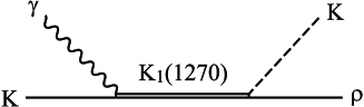
Figure 14: The same process as in fig. 12 but $\rho K$ in final state.

The same reaction as in ref. [21] but looking at $\rho K$ in the final state would have the advantage that the $K_{1}(1400)$ has a negligible decay rate to $\rho K$ [31]. Hence, the $K_{1}(1270)$ resonance would stand clean in the reaction. A similar analysis as done in ref. [21] could now be done in order to obtain the $K_{1}(1270)\to K^{0}\gamma$ decay width and would serve as a test of consistency of the result obtained in ref. [21]. However, from the perspective of the two pole scenario, this consistency is unlikely as we show below. Indeed, in fig. 13(b) we show the analogous to 13(a) for the $\rho K$ case. As we can see in the figure, the situation is reversed with respect to fig. 13(a), since now the dominant contribution comes from the pole B, instead of the pole A in the former case and the interference is now constructive. We think that the study of this reaction should in any case bring some additional information to the one done in ref. [21] and could shed some light into the issue of the two $K_{1}(1270)$ resonances.

5 Conclusions

We have evaluated the radiative decays of the low-lying axial-vector resonances into a pseudoscalar meson and a photon. For that purpose, we have extended a previous model originally devoted to the charged $a_{1}$ and $b_{1}$ radiative decay. In our model, the axial-vector resonances appear as dynamically generated through the interaction of a vector and a pseudoscalar meson, in the sense that they appear as poles in unphysical Riemann sheets of the scattering amplitudes without the need to include them as explicit degrees of freedom. Within this model the couplings of the axial-vector mesons to the different $VP$ channels can be easily obtained, even the relative signs which are crucial in the interferences of the present work. We evaluate the radiative decay widths by allowing the photon to be emitted from the decaying $VP$ product both at tree and one loop level contribution.

We make predictions for all these radiative decay widths and show that the final results are strongly affected by non-trivial interferences between different mechanisms, which are under control thanks to the knowledge of the couplings provided by the underlying unitary theory that generates dynamically the axial-vector resonances. This makes the final results to span a wide range of radiative widths from $0$ to $\sim 1$ MeV.

We have devoted special attention to the $K^{0}_{1}(1270)\to K^{0}\gamma$ decay for which there is only one experimental datum. In the underlying model of the present work this resonance has a double pole structure. We have discussed that, should this be the actual case in nature, it would have deep consequences in the experimental result since, in the experimental analysis, the usual one pole structure of the $K_{1}(1270)$ was considered. We have also proposed a related experiment using the Primakoff method with $\rho K$ in the final state instead of the $K^{*}\pi$ of ref. [21] in order to bring extra information on the issue of the two pole structure of the $K_{1}(1270)$ resonance. We argue that the result obtained for the radiative decay in both Primakoff experiments should be the same if there is only one pole. Yet, if there are two poles, the single pole analysis is inappropriate and would most probably lead to different results for the $K_{1}(1270)$ radiative width in the two experiments.

Further experimental measurements of the radiative decay widths of the axial-vector resonances would be welcome to shed more light on the nature of these resonances.

References

- [1] S. Capstick and W. Roberts, Prog. Part. Nucl. Phys. 45 (2000) S241.
- [2] T. Van Cauteren, J. Ryckebusch, B. Metsch and H. R. Petry, Eur. Phys. J. A 26 (2005) 339.
- [3] Y. Umino and F. Myhrer, Nucl. Phys. A 554 (1993) 593.
- [4] F. Myhrer, Phys. Rev. C 74 (2006) 065202.
- [5] L. Xiong, E. V. Shuryak and G. E. Brown, Phys. Rev. D 46 (1992) 3798.
- [6] K. Haglin, Phys. Rev. C 50 (1994) 1688.
- [7] G. Ecker, J. Gasser, A. Pich and E. de Rafael, Nucl. Phys. B 321 (1989) 311.
- [8] J. L. Rosner, Phys. Rev. D 23 (1981) 1127.
- [9] L. Roca, J. E. Palomar and E. Oset, Phys. Rev. D 70 (2004) 094006.
- [10] M. Doring, E. Oset and S. Sarkar, Phys. Rev. C 74 (2006) 065204.
- [11] M. Doring, Nucl. Phys. A 786 (2007) 164.
- [12] L. Roca, A. Hosaka and E. Oset, Phys. Lett. B 658 (2007) 17.
- [13] M. F. M. Lutz and E. E. Kolomeitsev, Nucl. Phys. A 730 (2004) 392.
- [14] L. Roca, E. Oset and J. Singh, Phys. Rev. D 72 (2005) 014002.
- [15] D. Jido, J. A. Oller, E. Oset, A. Ramos and U. G. Meissner, Nucl. Phys. A 725 (2003) 181.
- [16] C. Garcia-Recio, M. F. M. Lutz and J. Nieves, Phys. Lett. B 582 (2004) 49.
- [17] T. Hyodo, S. I. Nam, D. Jido and A. Hosaka, Phys. Rev. C 68 (2003) 018201.
- [18] V. K. Magas, E. Oset and A. Ramos, Phys. Rev. Lett. 95 (2005) 052301.
- [19] S. Prakhov et al. [Crystall Ball Collaboration], Phys. Rev. C 70 (2004) 034605.
- [20] L. S. Geng, E. Oset, L. Roca and J. A. Oller, Phys. Rev. D 75 (2007) 014017.
- [21] A. Alavi-Harati et al. [KTeV Collaboration], Phys. Rev. Lett. 89 (2002) 072001.
- [22] J. C. Nacher, E. Oset, H. Toki and A. Ramos, Phys. Lett. B 461 (1999) 299.
- [23] B. Borasoy, P. C. Bruns, U. G. Meissner and R. Nissler, Phys. Rev. C 72, 065201 (2005).
- [24] B. Borasoy, P. C. Bruns, U. G. Meissner and R. Nissler, arXiv:0709.3181 [nucl-th].
- [25] D. Gamermann, L. R. Dai and E. Oset, Phys. Rev. C 76 (2007) 055205.
- [26] A. E. Kaloshin, Phys. Atom. Nucl. 60 (1997) 1179 [Yad. Fiz. 60N7 (1997) 1306].
- [27] A. Faessler, T. Gutsche, V. E. Lyubovitskij and Y. L. Ma, Phys. Rev. D 76 (2007) 014005.
- [28] M. Napsuciale, E. Oset, K. Sasaki and C. A. Vaquera-Araujo, Phys. Rev. D 76 (2007) 074012.
- [29] J. E. Palomar, L. Roca, E. Oset and M. J. Vicente Vacas, Nucl. Phys. A 729 (2003) 743.
- [30] J. A. Oller and E. Oset, Phys. Rev. D 60 (1999) 074023.
- [31] W. M. Yao et al. [Particle Data Group], J. Phys. G 33 (2006) 1.
- [32] H. Primakoff, Phys. Rev. 81, 899 (1951); A. Halprin, C. M. Anderson, and H. Primakoff, Phys. Rev. 152, 1295 (1966).
- [33] C. Daum et al. [ACCMOR Collaboration], Nucl. Phys. B 187 (1981) 1.
- [34] D. M. Li and Z. Li, Eur. Phys. J. A 28 (2006) 369.
- [35] J. Babcock and J. L. Rosner, Phys. Rev. D 14 (1976) 1286.