The Renormalization Group Studies on Four Fermion Interaction Instabilities on Algebraic Spin Liquids

Abstract

We study the instabilities caused by four fermion interactions on algebraic spin liquids. Renormalization group (RG) is used for three types of previously proposed spin liquids on the square lattice: the staggered flux state of SU(2) spin system, the $\pi-$flux state of SU(4) spin system, and the $\pi-$flux state of SU(2) spin system. The low energy field theories of the first two types of spin liquids are QED3 with emerged SU(4) and SU(8) flavor symmetries , the low energy theory of the $\pi-$flux SU(2) spin liquid is the QCD3 with SU(2) gauge field and emergent Sp(4) (SO(5)) flavor symmetry. Suitable large-$N$ generalization of these spin liquids are discussed, and a systematic $1/N$ expansion is applied to the RG calculations. The most relevant four fermion perturbations are identified, and the possible phases driven by relevant perturbations are discussed.

I Introduction

Many algebraic spin liquid states have been proposed in 2+1 dimensional strongly correlated electronic systems. In these spin liquids neither the spin rotation symmetry nor the spatial discrete symmetry is broken, and the physical order parameters have algebraic correlations. The gapless excitations of the system include fractionalized spin excitations (the spinon) which are usually centered around isolated Dirac points, and in many cases also gapless gauge bosons. It is believed that when the number of gapless spinons with Dirac fermion spectrum is small enough, or when all the spinons are gapped, the gauge fields are confining. However, with large enough fermion numbers $N$, the system is believed to be described by a conformal field theory (CFT), with the fixed point gauge field coupling $e^{\ast 2}\sim 1/N$. Physics based on this conformal field theory at large-$N$ case has been studied in many references Hermele et al. (2005, 2004); Rantner and Wen (2002); Ran and Wen (2006), and it has been shown that the order parameters of various spin ordered patterns with different symmetry breaking can be all described as fermion bilinears at these critical spin liquids.

Reference Wen (2002) has provided us with a general formalism of studying the algebraic spin liquids. For spin-1/2 system, the lattice mean field variational Hamiltonian enjoys a SU(2) local gauge symmetry, on top of spin SU(2) global symmetry and all the lattice symmetries. The specific type of gauge symmetry that survives at low energy field theory depends on the choice of background mean field variational parameters, and the low energy gauge symmetries can be SU(2), U(1), or even $Z_{2}$. And since the $Z_{2}$ gauge field only introduces short range interaction between slave particles, the low energy long distance physics will not be modified by $Z_{2}$ gauge field. Thus we will only consider spin liquids with SU(2) and U(1) gauge field. Three types of spin liquids are of particular interest to us. The first two are the so-called staggered flux state of SU(2) spin system, and the $\pi-$flux state of SU(4) spin system Affleck and Marston (1988); Marston and Affleck (1989). Both states are expected to be described by the following action

$$L=\sum_{a=1}^{4N}\bar{\psi}_{a}\gamma_{\mu}(\partial_{\mu}+ia_{\mu})\psi_{a}+\cdots$$ (1)

The ellipses include all the other terms allowed by the symmetry or generalized symmetry transformations of the system. $\gamma_{\mu}$ with $\mu=1$, 2, 3 are just three Pauli matrices, which is special for $d=2$. Without the ellipses, action (1) describes a conformal field theory. Spin liquids described by (1) enjoy U(1) local gauge symmetry and SU(4N) flavor symmetry. For the staggered flux phase of SU(2) spin system, $N=1$, and for the $\pi-$flux phase of SU(4) spin system $N=2$. Since the SU(4N) flavor symmetry is larger than the physical symmetry, it is called the emergent flavor symmetry. As has been studied previously, all the fermion bilinears are forbidden by symmetry and projective symmetry transformations (PSG) Hermele et al. (2005), the only allowed local field theory terms which break the emergent flavor symmetry down to physical symmetries are four fermion interaction terms. Four fermion interactions violate the conformal invariance of actions (1), therefore it plays the role of instabilities of the CFT. In the limit of $N\rightarrow+\infty$, the scaling dimension of any four fermion terms is 4, which is obviously irrelevant. At finite $N$, whether these four fermion terms are relevant or not can be studied by explicitly calculating the $1/N$ corrections to the bare scaling dimension, and this will be one of the goals of the current paper.

Since all the four fermion terms are scalar under all the physical symmetry transformations, they should be mixed under RG flow. For the U(1) spin liquids described by (1), we will consider three types of four fermion terms. The first type of four fermion terms will preserve the SU(4N) emergent flavor symmetry. Due to the Pauli matrices nature of the Dirac matrices $\gamma_{\mu}$, there are only two terms in this category, and they will mix at the first order of $1/N$ expansion. We will show that these four fermion terms are likely to be irrelevant for even very small $N$, i.e. they will not create any instability. The second type of four fermion terms will break the SU(4N) symmetry down to Sp(4N) symmetry, this perturbation alone will be relevant at the CFT for small enough $N$, and it is likely that it will drive the system to another fixed point which describes a spin liquid with Sp(4N) symmetry and gapless U(1) gauge bosons Xu and Sachdev (2008). At $d=2$ there is only one term of this kind. The third type of four fermion terms break the flavor symmetry down to $\mathrm{SU(2N)\times SU(2)}$, and we will show that there is also a relevant linear combination. However with the presence of both the second and third type of four fermion terms, the symmetry of the system is only $\mathrm{Sp(2N)\times U(1)}$.

The physical meaning of these symmetry breaking can be understood as following: In the $N=1$ case, the physical symmetry is SU(2) ($\sim$ Sp(2)) spin symmetry plus all the lattice symmetries. It is also quite popular to interpret the four fold degenerate valence bond solid (VBS) states as an O(2) vector with $Z_{4}$ anisotropy, and the $Z_{4}$ symmetry breaking is possibly irrelevant at the critical point between Neel and VBS phases Senthil et al. (2004a, b); Lou et al. (2007). In the algebraic spin liquid formalism in this work, the VBS states are interpreted as fermion bilinears, and indeed transform as a planar vector under the U(1) group generator $\mu^{z}$. The $Z_{4}$ anisotropy of the O(2) vector should involve very high order of fermion interactions which are negligible at the CFT. Thus at the end of the chain of symmetry breaking, the symmetry is $\mathrm{Sp(2)\times U(1)}$, which is identical to the symmetry with the presence of both $\mathrm{SU(2N)\times SU(2)}$ four fermion terms and Sp(4N) four fermion terms ($N=1$). Thus driven by the $\mathrm{SU(2N)\times SU(2)}$ terms, the Sp(4N) fixed point is surrounded by phases with smaller symmetries, some of the phases will break the Sp(2N) spin symmetry, and some other phases may break the U(1) symmetry (the enlarged discrete symmetry). Therefore the Sp(4N) fixed point is a critical point (or multicritical point) between phases breaking completely different symmetries.

The $N=2$ case corresponds to the $\pi-$flux state of SU(4) spin system on the square lattice, and recent numerical results suggest that the $\pi-$flux state is a good candidate of the ground state of SU(4) Heisenberg model on the square lattice Assaad (2005). The SU(4) spin and pseudospin symmetry have been discussed in spin-orbit coupled systems Khaliullin and Maekawa (2000); Li et al. (1998) as well as spin-3/2 fermionic cold atom system Wu et al. (2003); Wu (2006, 2005). In spin-3/2 cold atom systems, since the particle density is very diluted, only the $s-$wave scattering should be considered. In this case, without fine-tuning any parameter, the system automatically enjoys Sp(4) (SO(5)) symmetry. And by tuning the ratio between the spin-2 scattering channel and spin-0 scattering channel, one can reach a critical point with SU(4) spin symmetry. In the spin-3/2 cold atom system at the vicinity of the SU(4) point, all the four fermion terms discussed above should exist as a perturbation to the $\pi-$flux state.

The third type of spin liquid we will discuss is the $\pi-$flux state of SU(2) spin system. This state is invariant under SU(2) local gauge transformation even at low energy field theory Wen (2002):

$$L=\sum_{l=1}^{3}\bar{\psi}\gamma_{\mu}(\partial_{\mu}-ia^{l}_{\mu}\sigma^{l})\psi+\cdots$$ (2)

$\sigma^{l}$ with $l=1,2$, $3$ are three Pauli matrices of the SU(2) gauge group. The flavor symmetry of this state has been shown to be Sp(4) Ran and Wen (2006). However, the SU(2) gauge field formalism makes the spin SU(2) symmetry inapparent Wen (2002). In reference Ran and Wen (2006), in order to make the SU(2) gauge symmetry and the SU(2) spin symmetry both apparent, the authors had to double the number of fermion components, but now the fermion multiplet suffers from a constraint: $\psi^{\ast}$ and $\psi$ are related through a unitary transformation. In order to do calculations without constraint, in this paper we will first introduce a Majorana fermion formalism for this $\pi-$flux state. In this formalism there are eight components of Majorana fermions with 2 Dirac species each, and the system enjoys an SO(8) flavor symmetry in the absence of gauge fluctuations. The SU(2) $\simeq$ SO(3) gauge group as well as Sp(4) $\simeq$ SO(5) flavor symmetry group are both subgroups of the SO(8) group. The Neel and VBS order parameters still form a vector representation of the SO(5) flavor group. In the large-$N$ generalization, the gauge group is still SU(2), and the flavor symmetry is Sp(2N), $N=2^{n}$, $n=1$, 2, $\cdots$. The large-$N$ generalization is applicable to the $\pi-$flux state of Sp(2N) spin models with $N=2^{n-1}$. Our calculations show that the SO(5) invariant four-fermion terms are not going to introduce any instability to the $\pi-$flux state, while the SO(5) breaking terms are relevant perturbations.

Our large-$N$ calculations have used some algebras and identities of SU(N), Sp(2N) Lie Algebras. The detailed analysis of the group theory and algebras will be summarized in the appendix. In section II and III we will study U(1) and SU(2) spin liquids respectively. In our calculations $1/N$ is the only small parameter used for expansion, and we do not assume $\epsilon=d-1$ to be small. Our loop integrals and field propagators are calculated in $d=2$, and a rigorous $\epsilon$ expansion should involve a general $d$ calculations. However, at general dimensions there are many more four fermion terms than the $d=2$ case, simply because at $d=2$ the three gamma matrices are Pauli matrices, the Fierz identity reduces the number of four fermion terms significantly, which is a very convenient property we want to make full use of. A formal rigorous general $d$ calculation is possible, we will leave it to the future study.

II spin liquids with U(1) gauge field

II.1 SU(4N) four fermion terms

The low energy field theory of the staggered flux state of SU(2) spin system and the $\pi-$flux state of SU(4) spin system are proposed to be described by CFT in equation (1). Four fermion interactions are one type of instabilities. As has been mentioned in the introductory section, we will focus on three types of four fermion terms. The first type contains two terms:

$$L_{1}=\frac{g_{1}}{4N\Lambda}(\bar{\psi}_{a}\psi_{a})^{2},\ L_{1}^{\prime}=\frac{g^{\prime}_{1}}{4N\Lambda}(\bar{\psi}_{a}\gamma_{\mu}\psi_{a})^{2}.$$ (3)

Hereafter the bracket denotes the trace in the Dirac space. The number $N$ and cut-off $\Lambda$ at the denominator is to guarantee both terms are at order of $N$ and the coefficients are dimensionless constants. In equation (3), $a=1,\cdots 4N$ is flavor indices, and we will focus on the case with $N=2^{n-1}$.

$L_{1}$ and $L_{2}$ are the only two four fermion terms which are both SU(4N) and Lorentz invariant. Throughout the paper we will only consider four fermion terms with Lorentz invariance, partly because a large class of interesting quantum critical points are $z=1$ theories with emergent Lorentz invariance; the Lorentz symmetry breaking effects in the kinetic terms of equation (1) have been considered in reference Hermele et al. (2005), and they were showed to be irrelevant. Several other SU(4N) invariant terms can be written down, for instance $(\bar{\psi}_{a}\psi_{b})(\bar{\psi}_{b}\psi_{a})$, $(\bar{\psi}_{a}\gamma_{\mu}\psi_{b})(\bar{\psi}_{b}\gamma_{\mu}\psi_{a})$, $\sum_{i=1}^{(4N)^{2}-1}(\bar{\psi}_{a}T^{i}_{ab}\psi_{b})(\bar{\psi}_{c}T^{i}_{cd}\psi_{d})$ and $\sum_{i=1}^{(4N)^{2}-1}(\bar{\psi}_{a}\gamma_{\mu}T^{i}_{ab}\psi_{b})(\bar{\psi}_{c}\gamma_{\mu}T^{i}_{cd}\psi_{d})$. Here $T^{i}$ are fundamental representations of SU(4N) algebra. However, using the Fierz identity of $\gamma_{\mu}$ matrices, and the identity (168) in the appendix, all these terms can be written as linear combinations of $L_{1}$ and $L_{2}$.

We will calculate the RG equation for the linear and quadratic order of the four fermion couplings. The first order corrections from $1/N$ expansion will be calculated for the linear term, and for the quadratic terms only the leading order of unity is calculated. Notice that when $g_{1}=g_{1}^{\prime}=0$ the system is at the CFT fixed point, so the point with zero four-fermion coupling is always a fixed point, despite the fact that gauge field fluctuations will generate effective four-fermion interactions Kaveh and Herbut (2005), the effects of these generated effective four-fermion interactions are included in diagram E and F of Fig. 2. At the CFT fixed point, the scaling dimensions of fermion bilinears have been calculated elsewhere Hermele et al. (2005, 2007). For instance,

$$\Delta(\bar{\psi}T_{a}\psi)=2-\frac{64}{3(4N)\pi^{2}},$$ (4)

(5)

$$\Delta(\bar{\psi}\psi)=2+\frac{128}{3(4N)\pi^{2}}.$$ (6)

These two fermion bilinears belong to different representations of the SU(4N) algebra, therefore their scaling dimensions should in principle differ from each other. Notice that the scaling dimension of conserved current $\bar{\psi}\gamma_{\mu}\psi$ and $\bar{\psi}\gamma_{\mu}T_{a}\psi$ do not gain any corrections from the $1/N$ expansion at this CFT fixed point, simply because the conservation law requires their scaling dimensions to be exactly 2.

The $1/N$ correction of scaling dimensions mainly comes from the dressed photon propagator Kim and Lee (1999):

$$G_{\mu\nu}(p)=\frac{16}{4Np}(\delta_{\mu\nu}-\frac{p_{\mu}p_{\nu}}{p^{2}}).$$ (7)

The Feynman diagrams which contribute to both $g_{1}$ and $g_{1}^{\prime}$ are listed in Fig. 1. Diagrams A and B are usually called the vertex and wavefunction renormalizations, which also contribute to fermion bilinears. Besides these one-loop diagrams, there are also two-loop diagrams (Fig. 2), which involve two photon propagators and one extra trace in the fermion flavor space, and hence also belongs to the $1/N$ order correction.

Figure 1: Feynman diagrams contribute to the linear orders in both Eqs. 11 and 16. The dashed lines are dressed photon propagators, and the full circles denote the trace in Dirac space.

Figure 2: Feynman diagrams which only contribute to the linear orders in Eqs. 11, but not in Eqs. 16.

Figure 3: Feynman diagrams which contribute to the quadratic order of the RG equations (11) and (16). Notice that since we only calculate to the order of unity in the quadratic terms, diagram G only contributes to equation (11) but not (16), and diagram H only contributes to equation (16) but not (11).

As already mentioned above, the quadratic terms in the equations are only calculated to the order of unity, the only Feynman diagram that contributes to this order is diagram G in Fig. 3, all the other diagrams will contain one extra $1/N$. After counting all the diagrams, the final RG equations are

$$\frac{dg_{1}}{d\ln l} = \left(-\epsilon-\frac{256}{3(4N)\pi^{2}}\right)g_{1}+\frac{64}{4N\pi^{2}}g_{1}^{\prime}-\frac{2}{\pi^{2}}g_{1}^{2},$$ (8)

$$\frac{dg_{1}^{\prime}}{d\ln l} = -\epsilon g^{\prime}_{1}+\frac{64}{3(4N)\pi^{2}}g_{1}+\frac{2}{3\pi^{2}}g_{1}^{\prime 2}.$$ (11)

Here $\epsilon=d-1=1$. At the fixed point $g_{1}=g_{1}^{\prime}=0$, the largest eigenvalue of flowing equations is $-1+1.39/(4N)$, which is always negative for any integer $N$. Thus we conclude that the The four fermion interactions which preserves SU(4N) symmetries are likely irrelevant for all $N$. And no stable fixed point is found at finite four fermion coupling. Another way of interpreting this result is that, the flavor symmetry preserving mass gap is not generated spontaneously, which is consistent with reference Kaveh and Herbut (2005).

II.2 Sp(4N) four fermion terms

The second type of four fermion terms will break SU(4N) symmetry to Sp(4N) symmetry Xu and Sachdev (2008). In Sp(4N) algebra there is a $4N\times 4N$ antisymmetric tensor $\mathcal{J}_{\alpha\beta}$ which satisfy

$$\mathcal{J}T^{a}_{\mathrm{sp(4N)}}\mathcal{J}=(T^{a}_{\mathrm{sp(4N)}})^{t},$$ (12)

(13)

$$\mathcal{J}T^{a}_{\mathrm{su(4N)/sp(4N)}}\mathcal{J}=-(T^{a}_{\mathrm{su(4N)/sp(4N)}})^{t}.$$ (14)

$T^{a}_{\mathrm{sp(4N)}}$ are elements of Sp(4N) algebra, and $T^{a}_{\mathrm{su(4N)/sp(4N)}}$ are elements in SU(4N) algebra but not Sp(4N) algebra. All the algebra elements for $N=2^{n-1}$ have been constructed in the appendix. The only four fermion term of this type is

$$L_{2}=\frac{g_{2}}{4N\Lambda}\mathcal{J}_{\alpha\gamma}\mathcal{J}_{\beta\sigma}(\bar{\psi}_{\alpha}\psi_{\beta})(\bar{\psi}_{\gamma}\psi_{\sigma}).$$ (15)

The other current-current interaction term $\mathcal{J}_{\alpha\gamma}\mathcal{J}_{\beta\sigma}(\bar{\psi}_{\alpha}\gamma_{\mu}\psi_{\beta})(\bar{\psi}_{\gamma}\gamma_{\mu}\psi_{\sigma})$ actually equals $L_{2}$ if one uses the Fierz identity of Dirac gamma matrices in $d=2$: $\gamma^{\mu}_{\alpha\beta}\gamma^{\mu}_{\gamma\sigma}=2\delta_{\alpha\sigma}\delta_{\beta\gamma}-\delta_{\alpha\beta}\delta_{\gamma\sigma}$.

The Feynman diagrams in Fig. 2 do not contribute to $g_{2}$, and the diagram H in Fig. 3 will contribute to the order of unity in the quadratic term in the RG equation:

$$\frac{dg_{2}}{d\ln l}=\left(-\epsilon+\frac{64}{4N\pi^{2}}\right)g_{2}-\frac{1}{3\pi^{2}}g_{2}^{2}.$$ (16)

This equation has fixed points at $g_{2}=0$ and $g_{2}=g_{2}^{\ast}=3\pi^{2}(-\epsilon+64/(4N\pi^{2}))$. At $d=2$ and $N=1$ we now find a result which is very different from the SU(4N) perturbations above. The $g_{2}=0$ fixed point is unstable with RG eigenvalue $0.621$, while the fixed point at $g_{2}=g_{2}^{\ast}>0$ is stable. Notice that the quadratic term in this equation is the only term with $\mathrm{O}(1/N^{0})$ coefficient, all the other nonlinear terms gain $1/N$ coefficient, thus the existence of this fixed point can be obtained from $1/N$ expansion with $N$ extrapolating back to $N=1$, even without assuming $\epsilon$ to be small. All the higher order terms in the $1/N$ expansions will only move the critical point by order of $1/N$ at most. Although now the fixed point value $g_{2}^{\ast}$ is of order unity, there is always a number $4N$ at the denominator of $g_{2}$, thus $g_{2}/(4N)$ can still be treated perturbatively close to the fixed point, as long as we do not encounter an extra factor of $4N$ in our calculation. Because $L_{2}$ is an pair-pair interaction term, no extra factor of $4N$ is gained in our calculation if we only calculate the scaling dimensions of terms like $\bar{\psi}T\psi$. The correction of $g_{2}^{\ast}$ to the scaling dimensions of $L_{1}$ and $L_{1}^{\prime}$ is also at the order of $1/(4N)$. For $N=2$, to the order of expansion done here, the fixed point with zero four-fermion terms is stable against $L_{2}$ perturbation, and the finite four-fermion coupling fixed point become instable. However, higher order $1/N$ corrections might change this result for $N=2$. Hereafter we will denote the critical value of $N$ as $N_{c1}$. One can also tune $N$ close to $N_{c1}$, and since $g_{2}^{\ast}$ is linear with $(N-N_{c1})/N$, at the vicinity of the critical $N$, $g_{2}^{\ast}$ can be treated perturbatively.

Figure 4: Feynman diagrams which contribute to the difference of scaling dimensions of fermion bilinears $\bar{\psi}T^{a}_{\mathrm{su(4N)/sp(4N)}}\psi$ and $\bar{\psi}T^{a}_{\mathrm{sp(4N)}}\psi$.

The scaling dimensions of all $(4N)^{2}-1$ fermion bilinears $\bar{\psi}T^{a}\psi$ ($T^{a}$ are SU(4N) generators) equal at the fixed point with $g_{i}=0$ which preserves the SU(4N) symmetry. The difference between the scaling dimensions of $\bar{\psi}T^{a}\psi$ and $\bar{\psi}\psi$ is from the diagrams similar to the ones in Fig. 3 Hermele et al. (2007) with two photon propagators and a trace in the fermion flavor space, which only contributes to fermion bilinear $\bar{\psi}\psi$. At the Sp(4N) symmetric fixed point, the scaling dimensions of fermion bilinears are classified as the representation of Sp(4N) algebra: $\bar{\psi}\psi$ and $\bar{\psi}T^{a}_{\mathrm{sp(4N)}}\psi$ form scalar and adjoint representations of Sp(4N) group respectively, the appendix proved that $\bar{\psi}T^{a}_{\mathrm{su(4N)/sp(4N)}}\psi$ also form a representation of Sp(4N) group at least for $N=2^{n-1}$. For instance, for the case with $n=1$, SU(4)/Sp(4) are just five Gamma matrices, which form a vector representation of SO(5) (Sp(4)) algebra. The scaling dimensions of fermion bilinears within the same representation are equal to each other.

If we assume $(N-N_{c1})/N$ and $1/N$ are of the same order, the scaling dimensions of the fermion bilinears at the Sp(4N) fixed point deviate from their value at the SU(4N) fixed point at the order of $1/N^{2}$, and requires a lot more calculations. But their differences at $1/N^{2}$ order can be calculated readily from diagrams in Fig. 4:

$$\Delta(\bar{\psi}T_{\mathrm{su(4N)/sp(4N)}}\psi)-\Delta(\bar{\psi}T_{\mathrm{sp(4N)}}\psi)=\frac{6g^{\ast}_{2}}{4N\pi^{2}}.$$ (17)

To obtain these results we have used the identities in equation (14). Without assuming $N-N_{c1}$ to be small, the scaling dimensions of fermion bilinears at the Sp(4N) fixed point can be calculated to the $1/N$ order as:

$$\Delta(\bar{\psi}T_{\mathrm{su(4N)/sp(4N)}}\psi)=2-\frac{64}{3(4N)\pi^{2}}+\frac{3g^{\ast}_{2}}{4N\pi^{2}},$$ (18)

(19)

$$\Delta(\bar{\psi}T_{\mathrm{sp(4N)}}\psi)=2-\frac{64}{3(4N)\pi^{2}}-\frac{3g^{\ast}_{2}}{4N\pi^{2}},$$ (20)

(21)

$$\Delta(\bar{\psi}\psi)=2+\frac{128}{3(4N\pi^{2})}+\frac{3g^{\ast}_{2}}{4N\pi^{2}}.$$ (22)

Notice that the diagrams in Fig. 4 are the only two diagrams which can contribute to the $1/N$ order of the scaling dimensions of fermion bilinears.

The Sp(4N) fixed point is located at the side with $g_{2}>0$. At the Sp(4N) fixed point, the modified linear order RG equation for $L_{1}$ and $L_{1}^{\prime}$ reads:

$$\frac{dg_{1}}{d\ln l} = \left(-\epsilon-\frac{256}{3(4N)\pi^{2}}-\frac{6g_{2}^{\ast}}{4N\pi^{2}}\right)g_{1}+\frac{64}{4N\pi^{2}}g_{1}^{\prime},$$ (23)

$$\frac{dg_{1}^{\prime}}{d\ln l} = -\epsilon g^{\prime}_{1}+\frac{64}{3(4N)\pi^{2}}g_{1}.$$ (26)

Thus at this Sp(4N) fixed point the SU(4N) perturbations $L_{1}$ and $L_{1}^{\prime}$ are even more irrelevant compared with at the SU(4N) fixed point.

When $g_{2}<0$ there is no stable fixed point and when $N$ is small enough the system will be driven to a state with only short range correlations. In this case the most favored state is likely to be the Sp(4N) singlet pairing state. In general the pairing amplitude $\mathcal{J}_{\alpha\beta}\langle\psi_{\alpha,i}\psi_{\beta,j}\rangle=C_{ij}$, and $C_{ij}$ is a symmetric tensor, $i$, $j$ are Dirac matrices indices. For convenience, we can choose the meanfield pairing amplitude to be $\mathcal{J}_{\alpha\beta}\langle\psi_{\alpha,i}\psi_{\beta,j}\rangle=C\delta_{ij}$, with constant $C$. This state breaks the U(1) gauge symmetry to $Z_{2}$ gauge symmetry because of the fermion pairing, the particle conservation of $\psi$ is also broken to conservation mod 2, but the Sp(4N) symmetry is preserved simply because the pairing is in the Sp(4N) singlet channel.

Using the identities (168) proved in the appendix, $L_{2}$ can also be written as

$$L_{2}=\sum_{a=1}^{8N^{2}-2N-1}\frac{g_{2}}{8N^{2}\Lambda}(\bar{\psi}T^{a}_{\mathrm{su(4N)/sp(4N)}}\psi)^{2}+\cdots$$ (27)

The ellipses are SU(4N) invariant terms $L_{1}$ and $L_{1}^{\prime}$. Thus when $g_{2}$ is negative and grow large, the system may also develop order $\langle\bar{\psi}T^{a}_{\mathrm{su(4N)/sp(4N)}}\psi\rangle\neq 0$, which breaks the Sp(4N) symmetry. The competition between the Sp(4N) symmetry breaking state and the Sp(4N) singlet pairing state requires further detailed analysis.

II.3 $\mathrm{SU(2N)\times\mathrm{SU(2)}}$ four fermion terms

The third type of four fermion terms are

$$L_{3}=\frac{g_{3}}{4N\Lambda}(\bar{\psi}_{\alpha a}\psi_{\alpha b})(\bar{\psi}_{\beta b}\psi_{\beta a}),$$ (28)

(29)

$$L_{3}^{\prime}=\frac{g^{\prime}_{3}}{4N\Lambda}(\bar{\psi}_{\alpha a}\gamma_{\mu}\psi_{\alpha b})(\bar{\psi}_{\beta b}\gamma_{\mu}\psi_{\beta a}).$$ (30)

Here $\alpha$ and $\beta$ are indices in the SU(2N) subspace, and $a$ and $b$ are indices in the SU(2) space. These two terms have other representations using identities proved in the appendix:

$$L_{3}=\frac{g_{3}}{8N\Lambda}(\bar{\psi}_{\alpha a}\vec{\mu}_{ab}\psi_{\alpha b})\cdot(\bar{\psi}_{\beta c}\vec{\mu}_{cd}\psi_{\beta d})+\cdots$$ (31)

(32)

$$L_{3}^{\prime}=\sum_{i=1}^{(2N)^{2}-1}-\frac{g_{3}^{\prime}}{4N^{2}\Lambda}(\bar{\psi}_{\alpha a}T^{i}_{\alpha\beta}\psi_{\beta a})(\bar{\psi}_{\gamma b}T^{i}_{\gamma\sigma}\psi_{\sigma b})+\cdots$$ (33)

Again the ellipses are $L_{1}$ and $L_{1}^{\prime}$. The RG equations of $g_{3}$ and $g_{3}^{\prime}$ will be mixed with $g_{1}$ and $g_{1}^{\prime}$ through the diagrams in Fig. 2. The final coupled RG equations are

$$\frac{dg_{1}}{d\ln l}=\left(-\epsilon-\frac{256}{3(4N)\pi^{2}}\right)g_{1}+\frac{64}{4N\pi^{2}}g_{1}^{\prime}$$ (34)

(35)

(36)

$$-\frac{64}{(4N)\pi^{2}}g_{3}-\frac{2}{\pi^{2}}g_{1}^{2},$$ (37)

(38)

(39)

$$\frac{dg_{1}^{\prime}}{d\ln l}=-\epsilon g^{\prime}_{1}+\frac{64}{3(4N)\pi^{2}}g_{1}+\frac{2}{3\pi^{2}}g_{1}^{\prime 2},$$ (40)

(41)

(42)

$$\frac{dg_{3}}{d\ln l}=\left(-\epsilon+\frac{128}{3(4N)\pi^{2}}\right)g_{3}+\frac{64}{4N\pi^{2}}g_{3}^{\prime}-\frac{1}{\pi^{2}}g_{3}^{2},$$ (43)

(44)

(45)

$$\frac{dg_{3}^{\prime}}{d\ln l}=-\epsilon g^{\prime}_{3}+\frac{64}{3(4N)\pi^{2}}g_{3}+\frac{1}{3\pi^{2}}g_{3}^{\prime 2}.$$ (46)

The perturbation with the highest scaling dimension at the fixed point with $g_{i}=0$ is

$$\lambda=-3/2g_{1}-1/2g_{1}^{\prime}+3g_{3}+g_{3}^{\prime},$$ (47)

the scaling dimension is $-\epsilon+64/(4N\pi^{2})$. When $N<N_{c2}=64/(4\pi^{2}\epsilon)$ coupling constant $\lambda$ is clearly relevant, but when $N=2$ at the first order calculation of $1/N$ expansion all the four fermion terms are irrelevant, the highest scaling dimension is about -0.189. However, higher order $1/N^{2}$ corrections might change this result. The critical $N_{c2}$ we calculated is consistent with the previous calculations in the context of spontaneous chiral symmetry breaking mass generation of QED3 Pisarski (1984); Appelquist et al. (1986, 1988); Kaveh and Herbut (2005).

Now let us assume $N<N_{c2}$, and after a long RG flow all the irrelevant couplings are negligible. Thus at low energy and long wavelength, $g_{3}\simeq g_{3}^{\prime}$, $g_{1}=g_{1}^{\prime}\simeq 0$, and the relevant coupling $\lambda=4g_{3}=4g_{3}^{\prime}$. Based on equation (33), positive relevant $\lambda$ tends to favor SU(2N) symmetry breaking order $\langle\bar{\psi}T^{a}_{\mathrm{su(2N)}}\psi\rangle\neq 0$, and negative relevant $\lambda$ tends to favor SU(2) symmetry breaking order $\langle\bar{\psi}\vec{\mu}\psi\rangle\neq 0$, which is usually referred to as chiral symmetry breaking mass generation. In this case the SU(4N) symmetric spin liquid becomes a critical point between two phases with different symmetry breaking.

As is shown in the appendix, with the presence of all the four fermion terms considered so far, the symmetry of the system is broken down to $\mathrm{Sp(2N)\times U(1)}$, mainly because neither the SU(2N) group nor the SU(2) group is a subgroup of Sp(4N). In the case of $N=1$ and staggered flux state, Sp(2N) subgroup is the SU(2) spin symmetry, and U(1) is the effective O(2) rotation of the planar vector formed by VBS order parameters. In the case of $N=2$ and $\pi-$flux state of SU(4) spin system, realized in spin-3/2 cold atoms, Sp(2N) subgroup is the unfine-tuned Sp(4) pseudospin symmetry.

At the first order $1/N$ expansion, two parameters have equally the highest scaling dimensions: $g_{2}$ and $\lambda=-3/2g_{1}-1/2g_{1}^{\prime}+3g_{3}+g_{3}^{\prime}$, but the equality between the two scaling dimensions are not protected by any symmetry. If $N<N_{c}=\mathrm{Min}[N_{c1},N_{c2}]$, both $g_{2}$ and $\lambda$ are relevant, and $g_{2}$ is likely to drive the system to a fixed point with Sp(4N) symmetry. Now let us focus on the vicinity of this Sp(4N) fixed point. If we take $\epsilon$ of order unity, the correction of the scaling dimension from fixed point value $g_{2}^{\ast}$ will be at order $1/N$, and $L_{3}$, $L_{3}^{\prime}$ will be mixing with many other terms with symmetry $\mathrm{Sp(2N)\otimes U(1)}$, the RG equations are rather complicated, but it is very unlikely that there is no relevant flowing eigenvector. Without detailed RG calculations, many results can be obtained intuitively. Based on the identity (168) proved in the appendix we have:

$$\sum_{a=1}^{2N(4N+1)}(\bar{\psi}T^{a}_{\mathrm{sp(4N)}}\psi)(\bar{\psi}T^{a}_{\mathrm{sp(4N)}}\psi)=$$ (48)

(49)

$$-2N\mathcal{J}_{\alpha\gamma}\mathcal{J}_{\beta\sigma}(\bar{\psi}_{\alpha}\psi_{\beta})(\bar{\psi}_{\gamma}\psi_{\sigma})+\cdots,$$ (50)

(51)

$$\sum_{a=1}^{8N^{2}-2N-1}(\bar{\psi}T^{a}_{\mathrm{su(4N)/sp(4N)}}\psi)(\bar{\psi}T^{a}_{\mathrm{su(4N)/sp(4N)}}\psi)=$$ (52)

(53)

$$2N\mathcal{J}_{\alpha\gamma}\mathcal{J}_{\beta\sigma}(\bar{\psi}_{\alpha}\psi_{\beta})(\bar{\psi}_{\gamma}\psi_{\sigma})+\cdots$$ (54)

As was discussed in the previous paragraph, without $g_{2}$, relevant $\lambda$ tends to favor either SU(2N) symmetry breaking order $\langle\bar{\psi}T^{a}_{\mathrm{su(2N)}}\psi\rangle\neq 0$ or SU(2) symmetry breaking order $\langle\bar{\psi}\vec{\mu}\psi\rangle\neq 0$, depending on the sign of $\lambda$. Notice that subalgebra $\mathrm{Sp(2N)\otimes 1}$ and $1\otimes\mu^{z}$ belong to Sp(4N), while $\mathrm{SU(2N)/Sp(2N)}$ and $1\otimes\mu^{x}$, $1\otimes\mu^{y}$ all belong to SU(4N)/Sp(4N). A positive $g_{2}$ will favor order $\langle\bar{\psi}T^{a}_{\mathrm{sp(2N)}}\psi\rangle$ over $\langle\bar{\psi}T^{a}_{\mathrm{su(2N)/sp(2N)}}\psi\rangle$ when $\lambda>0$; and also favors $\langle\bar{\psi}\mu^{z}\psi\rangle$ over $\langle\bar{\psi}\mu^{x}\psi\rangle$, $\langle\bar{\psi}\mu^{y}\psi\rangle$ with negative $\lambda$. Equation (22) also shows that order parameter $\bar{\psi}T^{a}_{\mathrm{sp(2N)}}\psi$ and $\bar{\psi}\mu^{z}\psi$ have stronger correlation and hence stronger tendency to order at the Sp(4N) fixed point compared with $\bar{\psi}T^{a}_{\mathrm{su(2N)}/\mathrm{sp(2N)}}\psi$ and $\bar{\psi}\mu^{x}\psi,\ \bar{\psi}\mu^{y}\psi$. Therefore the Sp(4N) fixed point is a critical point between Sp(2N) symmetry breaking order $\langle\bar{\psi}T^{a}_{\mathrm{sp(2N)}}\psi\rangle$ and order $\langle\bar{\psi}\mu^{z}\psi\rangle$. The RG flow diagram is shown in Fig. 5

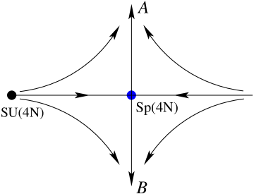
Figure 5: The RG flow when $N<N_{c}=\mathrm{Min}[N_{c1},N_{c2}]$, the horizontal axis is $g_{2}$, and the vertical axis is $\lambda$ in (47). At the Sp(4N) fixed point the order parameters with equally strongest correlations are $\bar{\psi}T^{a}_{\mathrm{sp(2N)}}\psi$ and $\bar{\psi}\mu^{z}\psi$, thus phase $A$ is most likely to be order $\langle\bar{\psi}T^{a}_{\mathrm{sp(2N)}}\psi\rangle$, and phase $B$ is most likely to be $\langle\bar{\psi}\mu^{z}\psi\rangle$. Notice that $\lambda$ is an RG eigenvector at the SU(4N) fixed point but not at the Sp(4N) fixed point, but phase A and B can be driven by $\lambda$ perturbation at the Sp(4N) fixed point.

From the first order $1/N$ expansion, $N_{c}$ is probably larger than 1. In the case of staggered flux state with $N=1$, the theories above show that with the four fermion terms considered so far, the Sp(4N) fixed point is a critical point between a SU(2) symmetry breaking state, and a state which breaks time reversal symmetry, but no spin or lattice translational symmetry is broken. However, the SU(2) symmetry breaking state is not the Neel order. The physical interpretations of these fermion bilinear order parameters can be found in reference Hermele et al. (2005). If the critical number $N_{c}$ is also greater than 2, as in the case of SU(4) $\pi-$flux state, the theory describes a critical point with Sp(8) symmetry between an SO(5) symmetry breaking phase with order parameter $\bar{\psi}\Gamma_{ab}\psi$, and a staggered chiral state which breaks translational symmetry and time reversal symmetry. Here $\Gamma_{ab}=\frac{1}{2i}[\Gamma_{a},\Gamma_{b}]$ are spinor representations of SO(5) (Sp(4)) group, and $\Gamma_{a}$ ($a$ = 1, 2 $\cdots$ 5) are five Gamma matrices.

When any of the fermion bilinear order is developed in the system, the fermionic spectrum is gapped. In the case of gapped matter field, the compact nature of the U(1) gauge boson is no longer negligible, and the monopole proliferation usually opens a gap for the gauge boson, and confine the gapped matter field. However, if the gapped fermions form a topological insulator, the U(1) gauge field is not necessarily confining. For instance, consider a Dirac fermion system with conserved fermion charge coupled with a compact U(1) gauge field, if the fermion gap $\bar{\psi}\psi$ is turned on, the system enters the quantum Hall state of spinons, and the Hall conductivity is half of the number of Dirac nodes. A Chern-Simons term is generated for the compact U(1) gauge field, in which case the monopole effect is suppressed Affleckb et al. (1990). This result can be understood physically as following: a monopole in 2+1 dimensional space-time annihilates/creates $2\pi$ flux of gauge field; however, an adiabatically inserted $2\pi$ gauge flux will trap one spinon due to the quantum Hall physics. And because of the conservation of the spinon number, the $2\pi$ flux cannot be created or annihilated freely.

In the order $\langle\bar{\psi}T^{a}_{\mathrm{sp(2N)}}\psi\rangle$, the sign of the fermion gap, i.e. the sign of the Hall conductivity depends on the Sp(2N) spin component. If a $2\pi-$flux is adiabatically inserted in the system, it will trap nonzero charge of $T^{a}_{\mathrm{sp(2N)}}$. In the past few years the quantum spin Hall effect (QSHE) has attracted a lot of attention, and many versions of QSHE models have been proposed, most of which are two copies of quantum Hall states with opposite Hall conductivities for spin up and down components Kane and Mele (2005a, b). Very recently the QSHE has been observed in experiments Bernevig et al. (2006); Koenig et al. (2007). In our case the state with $\langle\bar{\psi}T^{a}_{\mathrm{sp(2N)}}\psi\rangle$ is actually a Sp(2N) generalization of a quantum spin Hall model coupled with a compact U(1) gauge field. A nonzero Sp(2N) spin will be trapped by an adiabatically inserted $2\pi$ gauge flux due to the QSHE effect. Because of spin conservation, the monopole effect is again suppressed, thus in this state the spinons are gapped but not confined. However, the stability of the spin-filter edge states against the gapless U(1) gauge boson in the bulk requires more careful analysis. This type of states will be studied carefully in future Xu and Senthil (2008). In the order $\langle\bar{\psi}\mu^{z}\psi\rangle$, fermion gaps are opened for two Dirac valleys with opposite signs, i.e. the total charge Hall effect is zero. Also, since the O(2) rotation symmetry of $\mu^{x}$ and $\mu^{y}$ is broken down to $Z_{4}$ on the lattice, $\mu^{z}$ is not precisely a conserved quantity. Therefore the flux tunnelling is allowed, the monopoles are not suppressed, and the spinons are still confined due to the compact nature of the U(1) gauge field.

We want to point out that we have not yet exhausted all the four fermion terms allowed by the physical symmetry $\mathrm{Sp(2N)\times U(1)}$. Terms like $(\bar{\psi}_{\alpha a}\mu^{z}_{ab}\psi_{\alpha b})^{2}$, $\mathcal{J}^{\prime}_{\alpha\gamma}\mathcal{J}^{\prime}_{\beta\sigma}(\bar{\psi}_{\alpha a}\psi_{\beta a})(\bar{\psi}_{\gamma b}\psi_{\sigma b})$ and some others are all allowed. Here $\mathcal{J}^{\prime}$ is the antisymmetric tensor of the Sp(2N) algebra, and in the appendix we will prove that $\mathcal{J}=\mathcal{J}^{\prime}\otimes\mu^{x}$. Different four fermion terms will favor different ordered patterns. For instance, if $\mathrm{Sp(2N)\times U(1)}$ perturbation $\sum_{b}(\bar{\mathrm{\psi}}T^{b}_{\mathrm{sp(2N)}}\otimes\mu^{z}\psi)^{2}-\sum_{a=x}^{y}(\bar{\psi}\mu^{a}\psi)^{2}$ flows to the cut-off energy scale, it will drive a phase transition between the Sp(2N) Neel and VBS order.

III spin liquid with SU(2) gauge field

III.1 The Majorana fermion formalism

The $\pi-$flux state of SU(2) spin system on the square lattice enjoys SU(2) local gauge symmetries. The low energy effective theory of this state is

$$L=\sum_{a=1}^{2}\sum_{l=1}^{3}\bar{\psi}_{a}\gamma_{\mu}(\partial_{\mu}-ia^{l}_{\mu}\sigma^{l})\psi_{a}+\cdots$$ (55)

On the lattice, the variational parameter $U_{ij}$ hopping matrix is chosen to be: $U_{i,i+\hat{x}}=(-1)^{y}i\tau^{0}$, $U_{i,i+\hat{y}}=i\tau^{0}$, and the 2-site unit cell is chosen to be $(i,i+\hat{y})$. For this choice of gauge, the Dirac points are located at $(0,\pi/2)$ and $(\pi,\pi/2)$. We use $a$ and $b$ to denote this two Dirac node valleys. The Dirac gamma matrices are: $\gamma_{0}=\sigma^{2}$, $\gamma_{1}=-\sigma^{1}$, $\gamma_{2}=-\sigma^{3}$. It is believed that when the fermion number is large enough, action (55) describes a conformal field theory; when fermion number is small, the system is instable against confinement due to the antiscreening interaction between SU(2) gauge bosons Appelquist and Nash (1990); Appelquist et al. (1998). In this section we will discuss another type of instability of this conformal field theory driven by four fermion interactions.

The SU(2) gauge field is operating on $\psi=(\psi_{1},\psi_{2})^{T}=(f_{\uparrow},-f_{\downarrow}^{\dagger})^{T}$. However, physical spin SU(2) symmetry is not obvious in action (55). Since the charge density in equation (55) is actually spin density $S^{z}$, the charge current $\bar{\psi}\gamma_{\mu}\psi$ is not a singlet under spin SU(2) transformation. In order to resolve this problem, reference Ran and Wen (2006) enlarged the fermion space. However, after this treatment there is a constraint on the fermionic space: $\psi^{\ast}$ and $\psi$ are related through a unitary transformation, this makes the calculations based on action (55) inconvenient. In this section we will first introduce a Majorana fermion formalism for the $\pi-$flux state. In this Majorana fermion formalism both SU(2) gauge symmetry and SU(2) spin symmetry are both apparent, and there is no constraint on the fermion multiplet.

We define 8 component Majorana fermion multiplet $\chi$:

$$\chi_{111}=\mathrm{Re}(\psi_{1a}),\ \chi_{211}=\mathrm{Im}(\psi_{1a});$$ (56)

(57)

$$\chi_{121}=\mathrm{Re}(\psi_{2a}),\ \chi_{221}=\mathrm{Im}(\psi_{2a});$$ (58)

(59)

$$\chi_{112}=\mathrm{Re}(\psi_{1b}),\ \chi_{212}=\mathrm{Im}(\psi_{1b});$$ (60)

(61)

$$\chi_{122}=\mathrm{Re}(\psi_{2b}),\ \chi_{222}=\mathrm{Im}(\psi_{2b});$$ (62)

Each index of $\chi$ denotes a two-component space. The pauli matrices operating on the first, second and third two component space are denoted by $\tau^{a}$, $\sigma^{a}$ and $\mu^{a}$ respectively. If we ignore gauge fluctuations, this system enjoys an SO(8) symmetry, and all the symmetry transformations including the SU(2) gauge transformations are subgroups of this SO(8) group. We are going to write all the physical order parameters in terms of bilinears of the Majorana fermion $\chi T\chi$, the fermion statistics requires matrix $T$ to be antisymmetric.

Now we try to reformulate this theory in terms of $\chi$. In the Majorana fermion space, the three $\mathrm{SU(2)}_{gauge}$ matrices are

$$G_{3}=\tau^{2}\otimes\sigma^{x}\otimes 1,$$ (63)

(64)

$$G_{1}=\tau^{2}\otimes\sigma^{z}\otimes 1,$$ (65)

(66)

$$G_{2}=-1\otimes\sigma^{y}\otimes 1.$$ (67)

One can check that these three matrices, though mixing two different spaces, still form an SU(2) algebra. All the physical symmetry transformation should commute with this SU(2) algebra.

The bosonic version of our formalism actually realizes the beautiful second Hopf map. One way to study the O(5) Nonlinear Sigma model is to decompose the O(5) vector in terms of bosonic SU(4) spinors as $n^{a}=\Phi^{\dagger}\Gamma_{a}\Phi$, $\Gamma_{a}$ with $a=1$, 2, $\cdots 5$ are five Gamma matrices, and $\Phi$ is a four component complex bosonic spinor Demler and Zhang (1999). After this decomposition there is a redundant SU(2) gauge degrees of freedom, and since the four component complex boson $\Phi$ contains eight real components, the effective field theory of O(5) Nonlinear Sigma model with the Hopf term can be viewed as an O(8) sigma model coupled with SU(2) gauge field. With unit length constraint, the O(8) vector forms a manifold of seven dimensional sphere $\mathrm{S^{7}}$, and the theory describes a mapping: $\mathrm{S^{7}}/\mathrm{S^{3}}\rightarrow\mathrm{S^{4}}$, the $\mathrm{S^{3}}$ manifold is exactly the SU(2) group manifold, and $\mathrm{S^{4}}$ is the manifold formed by O(5) vector. This is a direct generalization of the first Hopf map which gives the $\mathrm{CP(1)}$ model, which is a popular way of rewriting the O(3) Nonlinear Sigma model Senthil et al. (2004a). This second Hopf map has been used to construct the 4 dimensional quantum Hall fluid Zhang and Hu (2001). The Wess-Zumino-Witten term of the O(5) Nonliear sigma model can also be derived from 2+1 dimensional Dirac fermion action Abanov and Wiegmann (2000).

Inspired by the second Hopf map, the flavor symmetry of our theory should be SO(5), in which the spin rotation symmetry should be contained. After some algebras, one can see that the spin transformation SU(2) algebra is

$$S^{z}=-\tau^{2}\otimes 1\otimes 1,$$ (68)

(69)

$$S^{x}=\tau^{1}\otimes\sigma^{y}\otimes 1,$$ (70)

(71)

$$S^{y}=\tau^{3}\otimes\sigma^{y}\otimes 1.$$ (72)

It is straightforward to check that $[S^{a},G_{b}]=0$. The gauge group generators in equation (67) and spin rotation generators in equation (72) together form an SO(4) algebra.

There are in total 10 elements in the SO(8) algebra which commute with the SU(2) gauge algebra, they are

$$S^{z}=-\tau^{2}\otimes 1\otimes 1,\ S^{x}=\tau^{1}\otimes\sigma^{y}\otimes 1,$$ (73)

(74)

$$S^{y}=\tau^{3}\otimes\sigma^{y}\otimes 1;\ -\tau^{2}\otimes 1\otimes\mu^{z},$$ (75)

(76)

$$-\tau^{2}\otimes 1\otimes\mu^{x};\ \tau^{1}\otimes\sigma^{y}\otimes\mu^{z},$$ (77)

(78)

$$\tau^{1}\otimes\sigma^{y}\otimes\mu^{x},\ \tau^{3}\otimes\sigma^{y}\otimes\mu^{z},$$ (79)

(80)

$$\tau^{3}\otimes\sigma^{y}\otimes\mu^{x},\ 1\otimes 1\otimes\mu^{y}.$$ (81)

These matrices are all antisymmetric, and form an SO(5) algebra. Besides these antisymmetric matrices, there are five symmetric matrices which form an vector representation of this SO(5) algebra:

$$\Gamma_{1}=\tau^{1}\otimes\sigma^{y}\otimes\mu^{y},\ \Gamma_{2}=\tau^{3}\otimes\sigma^{y}\otimes\mu^{y},$$ (82)

(83)

$$\Gamma_{3}=-\tau^{2}\otimes 1\otimes\mu^{y},\ \Gamma_{4}=1\otimes 1\otimes\mu^{x},$$ (84)

(85)

$$\Gamma_{5}=1\otimes 1\otimes\mu^{z}.$$ (86)

The first three matrices form a vector representation of spin SU(2) group, and it can be checked that $[G_{a},\Gamma_{i}]=0$ for all $a$ and $i$. Now one can construct fermion bilinears with SO(5) algebra constructed in equation (81) and the Gamma matrices constructed in equation (86). The physical interpretation of all the bilinears are summarized as following

$$\mathrm{Neel},\ n^{a}:\bar{\chi}\Gamma_{a}\chi,\ a=1,2,3;$$ (87)

(88)

$$\mathrm{ferromagnetic\ order},\ m^{a}:\ \bar{\chi}\gamma_{0}S^{a}\chi;$$ (89)

(90)

$$\mathrm{VBS_{x}}:\ \bar{\chi}\mu^{x}\chi,\ \mathrm{VBS_{y}}:\ \bar{\chi}\mu^{z}\chi;$$ (91)

(92)

$$\mathrm{chirality}:\ \bar{\chi}\chi;$$ (93)

(94)

$$\mathrm{staggered}\ \mathrm{chirality}:\ \bar{\chi}\gamma_{0}\mu^{y}\chi;$$ (95)

(96)

$$(-1)^{x}\vec{S}_{i}\times\vec{S}_{i+\hat{y}}:\ \bar{\chi}\gamma_{0}S^{a}\mu^{x}\chi,$$ (97)

(98)

$$(-1)^{y}\vec{S}_{i}\times\vec{S}_{i+\hat{x}}:\ \bar{\chi}\gamma_{0}S^{a}\mu^{z}\chi.$$ (99)

In the above equation, $\bar{\chi}=\chi^{T}\gamma_{0}$. These bilinears have exhausted all the elements in the SO(5) algebra and the $\Gamma_{a}$ matrices. All these fermion bilinears correspond to long wavelength fluctuations of certain order parameters on the lattice. The lattice version of spin chirality is $S_{1}\cdot(S_{2}\times S_{4})+S_{2}\cdot(S_{3}\times S_{1})+S_{3}\cdot(S_{4}\times S_{2})+S_{4}\cdot(S_{1}\times S_{3})$, $1$, $2$, $3$ and $4$ are sites on the four corners of a unit square, ordered clockwise.

The mean field choice of $U_{ij}$ apparently breaks the lattice symmetry, thus the lattice symmetry transformations should be combined with gauge transformations on the fermionic multiplet $\psi$, which is usually called the projective symmetry group (PSG). The complete PSG transformations combined with lattice symmetry are summarized as:

$$\mathrm{T_{x}}:\ 1\otimes 1\otimes\mu^{z},\ \mathrm{T_{y}}:\ 1\otimes 1\otimes\mu^{x},$$ (100)

(101)

$$\mathrm{P_{xs}}:\ \gamma_{1}\otimes\mu^{x},\ \mathrm{P_{xb}}:\ \gamma_{1}\otimes i\mu^{y},$$ (102)

(103)

$$\mathrm{P_{ys}}:\ \gamma_{2}\otimes\mu^{z},\ \mathrm{P_{yb}}:\ \gamma_{2}\otimes i\mu^{y},$$ (104)

(105)

$$\mathrm{P_{xy}}:\ (\gamma_{1}-\gamma_{2})\otimes(\mu^{x}+\mu^{z})/2,$$ (106)

(107)

$$\mathrm{T}:\ \gamma_{0}\otimes i\sigma^{y}\otimes\mu^{y}.$$ (108)

$\mathrm{T_{x}}$ and $\mathrm{T_{y}}$ are translations, $\mathrm{P_{xs}}$ and $\mathrm{P_{ys}}$ are site centered reflections, $\mathrm{P_{xb}}$ and $\mathrm{P_{yb}}$ are bond centered reflections, and $\mathrm{P_{xy}}$ is reflection along the line $x=y$, $\mathrm{T}$ is the time-reversal transformation. The time reversal transformation is an antiunitary operation, which transforms $i\rightarrow-i$. Therefore as long as matrix $T$ between $\chi T\chi$ contains $i$, it always gains an extra minus sign under time-reversal. For all the fermion bilinears in equation (99), Neel order parameter, ferromagnetic order parameter, chirality and staggered chirality are odd under time-reversal; VBS order parameters and staggered triplet bond order $(-1)^{i_{\mu}}\vec{S}_{i}\times\vec{S}_{i+\hat{\mu}}$ are even.

It is interesting to compare the fermion bilinear representations in the Majorana fermion formalism and the formalism in terms of $\psi$. Introducing $\Psi=(\psi,-i\sigma^{2}\psi^{\ast})^{T}$ and $\bar{\Psi}=\Psi^{\dagger}\gamma^{0}$ as in reference Ran and Wen (2006), the comparison between fermion bilinears in the $\chi$ language and $\psi$ language is listed below:

$$2\bar{\chi}\chi=\bar{\Psi}\Psi,\ 2\bar{\chi}\Gamma_{a}\chi=\bar{\Psi}\tilde{\Gamma}_{a}\Psi,$$ (109)

(110)

$$2\bar{\chi}\gamma_{\mu}G_{a}\chi=\bar{\Psi}\gamma_{\mu}\sigma^{a}\Psi,\ 2\bar{\chi}\gamma_{\mu}T^{a}\chi=\bar{\Psi}\gamma_{\mu}\tilde{T}^{a}\Psi,$$ (111)

(112)

$$\bar{\chi}\gamma_{\mu}\chi=\bar{\Psi}\gamma_{\mu}\Psi=0,\ \bar{\chi}G_{a}\chi=\bar{\Psi}\sigma^{a}\Psi=0,$$ (113)

(114)

$$\bar{\chi}T^{a}\chi=\bar{\Psi}\tilde{T}^{a}\Psi=0.$$ (115)

$G_{a}$ with $a=1,2,3$ are three matrices defined in equation (67), and $T^{a}$ are ten SO(5) algebra generators defined in equation (81). Notice that $\psi$ are $-i\sigma^{2}\psi^{\ast}$ both transform as spinors under gauge SU(2) group, $\sigma^{a}$ with $a=1$, 2, 3 are three gauge SU(2) Pauli matrices. The spin SU(2) transformation will mix $\psi$ and $-i\sigma^{2}\psi^{\ast}$, the Dirac node valley space is another direct product space. $\tilde{\Gamma}_{a}$ with $a=1,2,\cdots 5$ are five $4\times 4$ Gamma matrices operating on the spin space and Dirac node valley space:

$$\tilde{\Gamma}_{1}=\tilde{\sigma}^{1}\otimes\mu^{y},\ \tilde{\Gamma}_{2}=\tilde{\sigma}^{2}\otimes\mu^{y},\ \tilde{\Gamma}_{3}=\tilde{\sigma}^{3}\otimes\mu^{y},$$ (116)

(117)

$$\tilde{\Gamma}_{4}=\tilde{1}\otimes\mu^{x},\ \tilde{\Gamma}_{5}=\tilde{1}\otimes\mu^{z},$$ (118)

and $\tilde{T}^{a}$ with $a=1,2,\cdots 10$ are fundamental representations of ten $4\times 4$ $\mathrm{Sp(4)\simeq SO(5)}$ generators, which are also the commutators of $\tilde{\Gamma}_{a}$ matrices. Here $\tilde{\sigma}^{a}$ with $a=1,2,3$ are three spin SU(2) Pauli matrices which mix $\psi$ and $-i\sigma^{2}\psi^{\ast}$; $\mu^{a}$ with $a=x,y,z$ are three Pauli matrices operating on the Dirac node valley space.

Now the field theory of $\pi-$flux state in terms of Majorana fermions can be written as

$$L=\sum_{l=1}^{3}\bar{\chi}\gamma_{\mu}(\partial_{\mu}-ia_{\mu}^{l}G_{l})\chi+\cdots$$ (119)

Here $\bar{\chi}=\chi^{T}\gamma_{0}$. The ellipses should include all the four fermion terms allowed by PSG.

III.2 large-$N$ generalization and RG equations for four-fermion perturbations

The large-$N$ generalization of this problem can be achieved by increasing two-component fermionic spaces. The gauge field always only involves the first two 2-component spaces, and the gauge group is always SU(2). The details of large-$N$ generalization is in the appendix. Basically, for $n$ two-component fermionic spaces, the number of Majorana fermions is $N_{f}=2^{n}$, and the flavor symmetry which commute with the SU(2) gauge algebra is $\mathrm{Sp(4N)}$ with $N=2^{n-3}$. All the matrices in the particular representation of the Sp(4N) algebra are antisymmetric, and there are $8N^{2}-2N-1$ fermion bilinears $\bar{\chi}\Gamma_{a}\chi$ which form a representation of Sp(4N) algebra, $\Gamma_{a}$ are symmetric matrices. In the appendix we also proved that our large-$N$ generalization corresponds to the $\pi-$flux state of Sp(2N) spin system.

At the conformal field theory fixed point, the Majorana fermion propagators are

$$\langle\chi_{i,k}\bar{\chi}_{j,-k}\rangle=\delta_{ij}\frac{ik_{a}\gamma_{a}}{2k^{2}}.$$ (120)

This can be viewed as “half” fermion propagator. The dressed gauge field propagator after integrating out the fermions is

$$\langle a^{b}_{\mu}(q)a^{c}_{\nu}(-q)\rangle=\delta_{bc}\frac{32}{N_{f}q}(\delta_{\mu\nu}-\frac{q_{\mu}q_{\nu}}{q^{2}}).$$ (121)

In our physical situation $N_{f}=8$. The scaling dimensions of some fermion bilinears can be calculated readily:

$$\Delta(\bar{\chi}\chi)=2+\frac{256}{\pi^{2}N_{f}},$$ (122)

(123)

$$\Delta(\bar{\chi}\Gamma_{a}\chi)=2-\frac{128}{\pi^{2}N_{f}},$$ (124)

(125)

$$\Delta(\bar{\chi}\gamma_{\mu}T^{a}\chi)=2.$$ (126)

For all the Majorana fermion bilinears, the matrix between $\chi$ should be antisymmetric. One thing worth notice is that, the SU(2) gauge current $\bar{\chi}\gamma_{\mu}G_{a}\chi$ is no longer gauge invariant and hence has no well-defined scaling dimension. On the contrary, the scaling dimension of SU(2) gauge singlet current $\bar{\chi}\gamma_{\mu}T^{a}\chi$ gains no $1/N_{f}$ corrections.

The four fermion terms in the field theory should be invariant under all the symmetry transformations, thus they should be mixed under RG flow. The simplest four fermion terms are squares of Sp(4N) scalar fermion bilinears. To identify all the terms of this kind, we need to find a symmetric tensor $\mathcal{T}$ or antisymmetric tensor $\mathcal{J}$, which commute with gauge matrices $G^{a}$ and all the Sp(4N) flavor matrices. If these tensors exist, one can write down four fermion terms like

$$(\bar{\chi}\mathcal{T}\chi)^{2},\ (\bar{\chi}\gamma_{\mu}\mathcal{J}\chi)^{2},$$ (127)

(128)

$$\sum_{a=1}^{3}(\bar{\chi}\gamma_{\mu}\mathcal{T}G^{a}\chi)^{2},\ \sum_{a=1}^{3}(\bar{\chi}\mathcal{J}G^{a}\chi)^{2}.$$ (129)

In the physical case with $N=1$, the only symmetric tensor $\mathcal{T}$ one can find is the unit matrix, and there is no satisfactory antisymmetric $\mathcal{J}$. The representation of SO(5) in equation (81) belongs to a vector representation of SO(8) group and hence reducible, i.e. There are non-unit matrices commuting with all the matrices in (81). However, the gauge invariance criterion guarantees only the unit matrix $\mathcal{T}$ is satisfactory. Therefore the only two linear independent four fermion terms of this type are

$$L_{1}=\frac{g_{1}}{N_{f}\Lambda}(\bar{\chi}\chi)^{2},\ L_{1}^{\prime}=\sum_{a=1}^{3}\frac{g_{1}^{\prime}}{N_{f}\Lambda}(\bar{\chi}\gamma_{\mu}G_{a}\chi)^{2}.$$ (130)

In the original $\psi$ language, these two terms are $(\bar{\psi}\psi)^{2}$ and $\sum_{\mu,l}(\bar{\psi}\gamma_{\mu}\sigma^{l}\psi)^{2}$. Gauge singlet Current-current interaction $(\bar{\chi}\gamma_{\mu}\chi)^{2}$ is not allowed because of fermion statistics of $\chi$, i.e. in this theory there is no extra global U(1) symmetry. Both $L_{1}$ and $L_{1}^{\prime}$ are invariant under $\mathrm{SU(2)_{gauge}\otimes Sp(2N)}$ group, and they are mixed under RG flow at the linear order, i.e. the corrections from gauge field fluctuations. The Feynman diagrams that contribute to the anomalous dimensions are the same as the U(1) spin liquid case. The coupled RG equations for $g_{1}$ and $g_{1}^{\prime}$ are

$$\frac{dg_{1}}{d\ln l}=(-\epsilon-\frac{512}{\pi^{2}N_{f}})g_{1}+\frac{384}{\pi^{2}N_{f}}g_{1}^{\prime}-\frac{1}{\pi^{2}}g_{1}^{2},$$ (131)

(132)

(133)

$$\frac{dg_{1}^{\prime}}{d\ln l}=(-\epsilon+\frac{1024}{3\pi^{2}N_{f}})g_{1}^{\prime}+\frac{128}{3\pi^{2}N_{f}}g_{1}+\frac{1}{3\pi^{2}}g_{1}^{\prime 2}.$$ (134)

At the conformal field theory fixed point, the most relevant combination is $\lambda_{1}=0.44g_{1}+g_{1}^{\prime}$, with scaling dimension $-\epsilon+36.5/N_{f}$, with critical $N_{f,c1}=36.5$, which is much higher than the spin liquids with U(1) gauge field fluctuation considered in section II. At the physical case with $N_{f}=8$, this conformal field fixed point is very instable, and no stable fixed point is found at finite four fermion couplings. The irrelevant RG flow eigenvector is $-20.4g_{1}+g_{1}^{\prime}$, thus after long enough RG flow, $g_{1}^{\prime}\simeq 20.4g_{1}$, i.e. $L_{1}^{\prime}$ will dominate $L_{1}$ at low energy and long wavelength, thus the phase driven by these four fermion terms prefers to minimize $L_{1}^{\prime}$. $L_{1}^{\prime}$ is a SU(2) gauge current interaction, and gauge current $\bar{\chi}\gamma_{\mu}G_{a}\chi$ is not gauge invariant. Therefore the order driven by $L_{1}^{\prime}$ can break the SU(2) gauge symmetry. For instance, if the relevant flowing eigenvector $\lambda_{1}$ is negative, it will flow to a state which spontaneously generates a finite SU(2) gauge current on the lattice scale, and this gauge current will break the SU(2) gauge symmetry down to smaller gauge symmetries. If $\lambda_{1}>0$, the possible state driven by $\lambda_{1}$ is a SU(2) gauge singlet fermion paired state. Therefore if the Majorana fermion number $N$ is decreased from large enough value, two different instabilities will compete: the SU(2) gauge boson confinement tends to drive the system to an SU(2) gauge singlet ground state (the nature of this phase is not clear); while the four fermion interaction studied in the current work can drive the system to a state with broken SU(2) gauge symmetry.

When any fermion bilinear order $\langle\bar{\chi}T\chi\rangle$ is developed, the fermion spectrum is gapped. The screening of gapped fermions can no longer overcome the interactions between SU(2) gauge bosons, the gauge coupling flow will confine all the excitations with nonzero SU(2) gauge charge, all the excitations of this phase have to be SU(2) gauge singlet. However, if the SU(2) gauge symmetry is broken spontaneously by the relevant four fermion terms, the residual gauge field fluctuation may or may not be confining, depending on the gauge group. If the residual gauge group is $Z_{2}$, the gapped spinons can be still deconfined; if the residual gauge group is U(1), for instance when a uniform gauge current $\bar{\chi}\gamma_{\mu}G^{a}\chi$ is generated, the monopole fluctuation will confine the spinons, and the specific ground state order pattern is determined by the quantum number of monopoles. Notice that although both $L_{1}$ and $L_{1}^{\prime}$ are SO(5) invariant, the SO(5) symmetry can be broken by the quantum number of proliferating monopoles. A full analysis of the monopole quantum number is not yet accomplished.

In the appendix we showed that the SU(2) gauge invariant formalism is only exact for Sp(2N) Hamiltonian with $J_{2}=0$ in equation (202). When $J_{2}\neq 0$ the system only enjoys the U(1) gauge symmetry, and if $J_{2}=J_{1}$ the spin model becomes SU(2N) invariant, and the $\pi-$flux state is described by QED3. Now let us consider turning on a small $J_{2}$ perturbation on the $\pi-$flux state of Sp(2N) spin Hamiltonian with only $J_{1}$ in equation (202), this perturbation will generate four-fermion perturbation

$$L_{2}=\frac{g_{2}}{N_{f}\Lambda}\{2(\bar{\chi}\gamma_{\mu}G^{3}\chi)^{2}-(\bar{\chi}\gamma_{\mu}G^{1}\chi)^{2}-(\bar{\chi}\gamma_{\mu}G^{2}\chi)^{2}\}.$$ (135)

$L_{2}$ is one component of the $d-$wave vector under gauge SU(2) group. Since $L_{2}$ belongs to a different representation under SU(2) gauge group from $L_{1}$ and $L_{1}^{\prime}$, the linear RG equation of $L_{2}$ will not be mixed with $L_{1}$ and $L_{1}^{\prime}$. Also since $\bar{\chi}G^{a}\chi$ vanishes due to fermion statistics, $L_{2}$ itself is an eigenvector under linearized RG flow to the first order of $1/N$ expansion.

The RG equation for $L_{2}$ reads

$$\frac{dg_{2}}{d\ln l}=(-\epsilon+\frac{256}{3\pi^{2}N_{f}})g_{2}+\frac{1}{3\pi^{2}}g_{2}^{2}.$$ (136)

Now the situation is similar to the $L_{2}$ considered in the U(1) spin liquid case. The scaling dimension of $g_{2}$ is $-\epsilon+256/(3\pi^{2}N_{f})$, and for $N<N_{f,c2}=256/(3\pi^{2})=8.7$, $L_{2}$ will drive the system to a fixed point with a finite $g_{2}$. At the fixed point of finite $g_{2}$, the SU(2) gauge symmetry is broken down to U(1) gauge symmetry generated by $G^{3}$, thus this fixed point is very analogous to the fixed point with finite $L_{2}$ discussed in the section II. The critical value of $N_{f,c2}$ from the first order $1/N_{f}$ expansion is slightly larger than 8, and for the $\pi$-flux state of the Sp(4) spin model with $N_{f}=16$, $L_{2}$ will not bring an instability to the state, and the finite $g_{2}$ fixed point becomes a critical point.

So far we have preserved the Sp(2N) flavor symmetry, which is larger than the physical symmetry. As is discussed in the appendix, our large-$N$ generalization is applicable to the $\pi-$flux state of Sp(2N) spin model with $N=2^{n-1}$. Therefore four fermion terms which break the emergent flavor symmetry down to physical symmetries certainly exist in the field theory. Let us assume the total number of 2-component fermion space is $k+1$, two terms of this kind are

$$L_{3}=\frac{g_{3}}{N_{f}\Lambda}\sum_{a}\{2(\bar{\chi}T^{a}_{k}\otimes\mu^{y}\chi)^{2}-(\bar{\chi}\mu^{x}\chi)^{2}-(\bar{\chi}\mu^{z}\chi)^{2}]\},$$ (137)

(138)

$$L^{\prime}_{3}=\frac{g^{\prime}_{3}}{N_{f}\Lambda}\sum_{a,b}\{2(\bar{\chi}T^{a}_{k}\otimes\mu^{y}\gamma_{\mu}G^{b}\chi)^{2}-\sum_{i=x,z}(\bar{\chi}\mu^{i}\gamma_{\mu}G^{b}\chi)^{2}]\}.$$ (139)

Notice that fermion bilinear $\bar{\chi}T^{a}_{k}\otimes\mu^{y}\chi$ is the large-$N$ analogue of the Neel order parameter, $\bar{\chi}\mu^{x}\chi$ and $\bar{\chi}\mu^{z}\chi$ are the large-$N$ analogue of the VBS order parameters, therefore a relevant $L_{3}$ will favor either Neel or VBS phase depending on the sign. The coupled linear RG equations for $g_{3}$ and $g_{3}^{\prime}$ read

$$\frac{dg_{3}}{d\ln l}=(-\epsilon+\frac{256}{\pi^{2}N_{f}})g_{3}+\frac{384}{\pi^{2}N_{f}}g_{3}^{\prime},$$ (141)

(142)

$$\frac{dg^{\prime}_{3}}{d\ln l}=(-\epsilon+\frac{256}{\pi^{2}N_{f}})g^{\prime}_{3}+\frac{128}{3\pi^{2}N_{f}}g_{3}.$$ (143)

The most relevant eigenvalue of the RG flow is $-\epsilon+38.9/N_{f}$, the critical value of $N_{f,c3}$ is $38.9$, which is slightly higher than the critical value of $N_{f,c1}$ for $L_{1}$ and $L_{1}^{\prime}$ based on our first order $1/N$ expansion. If $N_{f,c3}$ is indeed higher than $N_{f,c1}$, when $N_{f,c1}<N_{f}<N_{f,c3}$ the $\pi-$flux state is a critical point between Neel order $\bar{\chi}T^{a}_{k}\otimes\mu^{y}\chi$ and VBS order. The classification of the four-fermion terms is worked on elsewhere ran (2008).

IV concluding remarks

In this work we studied the effects of four fermion interactions as one type of instabilities on several interesting algebraic spin liquids. The RG calculations show the gauge field fluctuation will generally enhance the relevance of the four fermion interactions, except for one particular pair which preserves the SU(4N) emergent flavor symmetry in the spin liquids with U(1) gauge field. For the $N=1$ U(1) spin liquid, several four fermion terms are relevant at the spin liquid. The four fermion term which breaks the SU(4N) symmetry to Sp(4N) symmetry will likely drive the system to a fixed point with finite coupling which describes a spin liquid with Sp(4N) symmetry, which is a critical point between phases with smaller symmetries. For the $N=2$ case, all the four fermion terms are irrelevant at the first order $1/N$ correction. The $\pi-$flux state with SU(2) gauge field is more vulnerable against four fermion terms, the critical fermion number is much higher compared with U(1) spin liquids. The specific phases driven by relevant four fermion couplings were conjectured in this paper, but more detailed calculation is required to determine which phases are most favorable ones.

Another physical system with low energy Dirac fermion excitations is graphene, where the Dirac nodes locate at the corners of the Brillouin zone. There are two flavors of Dirac fermions coming from the two inequivalent corners of the Brillouin zone, and another two flavors from the spin degeneracy. Thus in this system the total number of Dirac fermions is $N=4$. The difference between this case and our spin liquids is that, there is no fluctuating gauge field in graphene, except for a static Coulomb interaction. Due to the apparent Lorentz symmetry breaking of the Coulomb interaction, the fermi velocity will flow under RG. The effects of four fermion terms in graphene have been studied in reference Drut and Son (2007).

It has been suggested that the deconfine critical point between the Neel and VBS is of enlarged SO(5) symmetry Senthil and Fisher (2006); Sandvik (2007); Melko and Kaul (2007), and the Neel and VBS order parameters together form an SO(5) vector Tanaka and Hu (2005). The deconfined critical point between the Neel and VBS order is conjectured to be a liquid phase of O(5) Nonlinear sigma model with a Wess-Zumino-Witten term. A liquid phase with enlarged SO(5) symmetry can exclude many possible relevant perturbations. In our theory, SO(5) symmetry has appeared here and there, and both in the U(1) spin liquids and the SU(2) spin liquid the Neel and VBS order parameters form a five component SO(5) vector. Although we have not completely identified the deconfine critical point in our theory, our formalism especially the Majorana fermion formalism of SU(2) $\pi-$flux state is still a promising approach to locate the deconfine critical point, simply because of the beautiful second Hopf map. To do this, one needs to find a fixed point with Sp(4) flavor symmetry and only one relevant four fermion interaction which breaks Sp(4) symmetry down to $\mathrm{SU(2)\otimes U(1)}$. The fixed point with Sp(4) symmetry we identified in the U(1) spin liquid section has one extra U(1) gauge symmetry compared with the O(5) Nonlinear sigma model description of the deconfined critical point Senthil and Fisher (2006), which in the dual language corresponds to the conservation of gauge flux.

It is interesting to generalize the field theory of the deconfined critical point to larger spin systems, and one can approach these deconfined critical points from large-$N$ version of the spin liquids studied in this work. First of all, the VBS order can be naturally generalized to systems with Sp(2N) symmetry simply because two Sp(2N) particles with fundamental representation can form a Sp(2N) singlet through antisymmetric matrix $\mathcal{J}$: $\mathcal{J}_{\alpha\beta}\psi^{\dagger}_{\alpha}\psi^{\dagger}_{\beta}$. The Neel order parameter spans an adjoint representation of the Sp(2N) group. The large-$N$ formalism of spin liquids in our current paper shows that the smallest simple group with $\mathrm{Sp(2N)\otimes U(1)}$ subgroup is Sp(4N). Therefore if an unfine-tuned second order transition between Sp(2N) Neel and VBS order exists, this critical point can enjoy enlarged Sp(4N) symmetry.

V Appendix

V.1 Construction of fundamental representations of Sp(4N) algebra with $N=2^{n}$

In this appendix we will construct the fundamental representations of SU(4N) and Sp(4N) algebras with $N=2^{n}$. All the results will be proved by induction, thus we will first present all the results, which are obviously true for $n=0$; later we will assume they are also valid for $n=k$, the same results for $n=k+1$ can be proved directly from our construction of SU(4N) and Sp(4N) algebras.

1st, SU(4N) algebra contains subalgebra $\mathrm{SU(2N)\otimes SU(2)}$, the whole fundamental representation of SU(4N) algebra can be constructed from the fundamental representations of its SU(2N) subalgebra and SU(2) subalgebra. All the SU(4N) algebra elements can be written as

$$T_{a}\otimes\mu^{i},\ T_{a}\otimes 1,\ 1\otimes\mu^{i}.$$ (144)

$T_{a}$ with $a=1$, 2 $\cdots$ $(2N)^{2}-1$ are fundamental representations of all the elements in SU(2N) algebra, and $\mu^{i}$ with $i=1$ 2, 3 are three SU(2) Pauli matrices.

2nd, SU(2N) algebra has an Sp(2N) subalgebra, which satisfy

$$\mathcal{J}_{\mathrm{2N}}T^{a}_{\mathrm{sp(2N)}}\mathcal{J}_{\mathrm{2N}}=(T^{a}_{\mathrm{sp(2N)}})^{t}.$$ (145)

Here $\mathcal{J}_{\mathrm{2N}}$ is a $2N\times 2N$ antisymmetric matrix.

3rd, all the SU(2N) elements in SU(2N)/Sp(2N) satisfy

$$\mathcal{J}_{\mathrm{2N}}T^{a}_{\mathrm{su(2N)/sp(2N)}}\mathcal{J}_{\mathrm{2N}}=-(T^{a}_{\mathrm{su(2N)/sp(2N)}})^{t}.$$ (146)

4th, all the elements in SU(2N)/Sp(2N) form a representation of Sp(2N); or more precisely, fermion bilinear $\bar{\psi}\Gamma^{a}_{\mathrm{su(2N)/sp(2N)}}\psi$ spans a representation of Sp(2N) algebra. To prove this, one has to show that

$$[T^{a}_{\mathrm{sp(2N)}},T^{b}_{\mathrm{su(2N)/sp(2N)}}]\in\mathrm{SU(2N)/Sp(2N)}.$$ (147)

The meaning of the equation above is that, the commutator between any element in SU(2N)/Sp(2N) and any element in Sp(2N) belongs to SU(2N)/Sp(2N).

5th, all the elements in SU(2N) algebra satisfy following relations:

$$[T^{a}_{\mathrm{sp(2N)}},T^{b}_{\mathrm{sp(2N)}}]\in\mathrm{Sp(2N)},$$ (148)

(149)

$$[T^{a}_{\mathrm{sp(2N)}},T^{b}_{\mathrm{su(2N)/sp(2N)}}]\in\mathrm{SU(2N)/Sp(2N)},$$ (150)

(151)

$$[T^{a}_{\mathrm{su(2N)/sp(2N)}},T^{b}_{\mathrm{su(2N)/sp(2N)}}]\in\mathrm{Sp(2N)},$$ (152)

(153)

$$\{T^{a}_{\mathrm{sp(2N)}},T^{b}_{\mathrm{sp(2N)}}\}\in\mathrm{SU(2N)/Sp(2N)},$$ (154)

(155)

$$\{T^{a}_{\mathrm{sp(2N)}},T^{b}_{\mathrm{su(2N)/sp(2N)}}\}\in\mathrm{Sp(2N)},$$ (156)

(157)

$$\{T^{a}_{\mathrm{su(2N)/sp(2N)}},T^{b}_{\mathrm{su(2N)/sp(2N)}}\}\in\mathrm{SU(2N)/Sp(2N)}.$$ (158)

(159)

6th, for the fundamental representations of SU(2N) and Sp(2N) algebras, following identities are satisfied:

$$\sum_{a=1}^{(2N)^{2}-1}T^{a}_{\mathrm{su(2N)},\alpha\beta}T^{a}_{\mathrm{su(2N)},\gamma\sigma}=2N\delta_{\alpha\sigma}\delta_{\beta\gamma}-\delta_{\alpha\beta}\delta_{\gamma\sigma},$$ (160)

(161)

$$\sum_{a=1}^{N(2N+1)}T^{a}_{\mathrm{sp(2N)},\alpha\beta}T^{a}_{\mathrm{sp(2N)},\gamma\sigma}$$ (162)

(163)

$$=N\delta_{\alpha\sigma}\delta_{\beta\gamma}-N\mathcal{J}_{\alpha\gamma}\mathcal{J}_{\beta\sigma},$$ (164)

(165)

$$\sum_{a=1}^{2N^{2}-N-1}T^{a}_{\mathrm{su(2N)/sp(2N)},\alpha\beta}T^{a}_{\mathrm{su(2N)/sp(2N)},\gamma\sigma}$$ (166)

(167)

$$=N\delta_{\alpha\sigma}\delta_{\beta\gamma}+N\mathcal{J}_{\alpha\gamma}\mathcal{J}_{\beta\sigma}-\delta_{\alpha\beta}\delta_{\gamma\sigma}.$$ (168)

All these identities have been used in the main text of our paper.

Now the Sp(4N) algebra which is a subalgebra of SU(4N) can be constructed as

$$T^{a}_{\mathrm{sp(2N)}}\otimes\mu^{x},\ T^{a}_{\mathrm{sp(2N)}}\otimes\mu^{y},\ T^{a}_{\mathrm{sp(2N)}}\otimes 1,$$ (169)

(170)

$$1\otimes\mu^{z},\ T^{a}_{\mathrm{su(2N)/sp(2N)}}\otimes\mu^{z}.$$ (171)

There are in total 2N(4N+1) elements in (171). All these matrices satisfy

$$\mathcal{J}_{\mathrm{4N}}T^{a}_{\mathrm{sp(4N)}}\mathcal{J}_{\mathrm{4N}}=(T^{a}_{\mathrm{sp(4N)}})^{t},$$ (172)

(173)

$$\mathcal{J}_{4N}=\mathcal{J}_{\mathrm{2N}}\otimes\mu^{x}.$$ (174)

Meanwhile, All the elements in SU(4N) constructed in (144) but not in Sp(4N) constructed in equation (171) are

$$1\otimes\mu^{x},\ 1\otimes\mu^{y},$$ (175)

(176)

$$T^{a}_{\mathrm{su(2N)/sp(2N)}}\otimes\mu^{x},\ T^{a}_{\mathrm{su(2N)/sp(2N)}}\otimes\mu^{y},$$ (177)

(178)

$$T^{a}_{\mathrm{su(2N)/sp(2N)}}\otimes 1,\ T^{a}_{\mathrm{sp(2N)}}\otimes\mu^{z}$$ (179)

There are in total $\mathrm{8N^{2}-2N-1}$ elements in equation (179).

All the equations from (168) to (174) are valid for SU(4) and Sp(4) algebras. Let us assume these results are true for $n=k$, then for $n=k+1$, equations (174), (146), (147), (159) and (168) can be checked directly through constructions in equations (144), (171) and (179), and by using the assumptions made for $n=k$. The calculations are tedious but straightforward.

We have proved that the fundamental representation of SU(4N) algebra with $N=2^{n}$ can all be constructed by Pauli matrices, thus $(T^{a}_{\mathrm{su(4N)}})^{2}=1$. Because of this and equation (147), vector $n^{a}=(\bar{\psi}T^{a}_{\mathrm{su(4N)/sp(4N)}}\psi)$ rotates under Sp(4N) group, while keeping the length $\sum_{a}(n^{a})^{2}$ constant.

One can see that the SU(2N) subalgebra of SU(4N) does not completely belong to Sp(4N) constructed in equation (171). Instead, only the Sp(2N) subalgebra is a subalgebra of Sp(4N), and the SU(2N)/Sp(2N) part belongs to SU(4N)/Sp(4N). Meanwhile, the subalgebra SU(2) which commute with SU(2N) is not a subalgebra of Sp(4N) either, only element $\mu^{z}$ which generates U(1) rotation belongs to Sp(4N). Therefore when the $\mathrm{SU(2N)\otimes SU(2)}$ and $\mathrm{Sp(4N)}$ four fermion terms both exist, the symmetry of the system is actually only $\mathrm{Sp(2N)\otimes U(1)}$.

V.2 Large-$N$ generalization of the $\pi-$flux state of SU(2) spin model

In this subsection we will show that for Majorana fermions with $n+1$ two-component space coupled with SU(2) gauge field, the flavor symmetry is Sp(4N) with $N=2^{n-2}$. In our paper we showed that for $n=1$ and $2$, the flavor symmetry is SO(3)$\simeq$Sp(2) and SO(5)$\simeq$Sp(4) respectively, and for $n=2$ there are 5 symmetric matrices which make fermion bilinears $\bar{\chi}\Gamma_{a}\chi$ span a representation of Sp(4). We will try to generalize these results to larger number $n$. For $n=k$, let us first denote the Sp(2N) algebra elements as $T^{a}_{k}$, and denote the space spanned by the symmetric matrices as $\Gamma_{\mathrm{sp(2N),k}}$; and second, assume for $n=k$, following algebra is valid:

$$[T^{a}_{k},T^{b}_{k}]\in\mathrm{Sp(2N)}_{k},\ [\Gamma^{a}_{k},\Gamma^{b}_{k}]\in\mathrm{Sp(2N)}_{k},$$ (180)

(181)

$$[T^{a}_{k},\Gamma^{b}_{k}]\in\Gamma_{\mathrm{sp(2N)},k},\ \{T^{a}_{k},T^{b}_{k}\}\in\Gamma_{\mathrm{sp(2N)},k},$$ (182)

(183)

$$\{\Gamma^{a}_{k},\Gamma^{b}_{k}\}\in\Gamma_{\mathrm{sp(2N)},k},\ \{T^{a}_{k},\Gamma^{b}_{k}\}\in\mathrm{Sp(2N)}_{k}.$$ (184)

These algebras are valid for the simplest case with $n=1$ and $n=2$.

Now we construct Sp(2N) and $\Gamma_{\mathrm{sp(2N)}}$ for $n=k+1$ as following:

$$\mathrm{Sp(2N)}_{k+1}:$$ (185)

(186)

$$T^{a}_{k}\otimes\mu^{x},\ T^{a}_{k}\otimes\mu^{z},\ \Gamma^{a}_{k}\otimes\mu^{y},\ T^{a}_{k}\otimes 1,\ 1\otimes\mu^{y};$$ (187)

(188)

$$\Gamma_{\mathrm{sp(2N)},k+1}:$$ (189)

(190)

$$\Gamma^{a}_{k}\otimes\mu^{x},\ \Gamma^{a}_{k}\otimes\mu^{z},\ T^{a}_{k}\otimes\mu^{y},\ \Gamma^{a}_{k}\otimes 1,$$ (191)

(192)

$$1\otimes\mu^{x},\ 1\otimes\mu^{z}.$$ (193)

$\mu^{a}$ are Pauli matrices in the new two component space. Although for this representation of Sp(2N) algebra there is no antisymmetric matrices $\mathcal{J}$ which satisfies $\mathcal{J}T^{a}\mathcal{J}=(T^{a})^{t}$, the construction in equation (193) is exactly the same as the construction in (171) in the previous section, except for exchanging $\mu^{z}$ and $\mu^{y}$, thus the algebra in equation (193) is Sp(2N). There are in total $N(2N+1)$ elements in Sp(2N), and $2N^{2}-N-1$ elements in $\Gamma_{\mathrm{sp(2N)}}$. The validity of algebra in (184) for $n=k+1$ can be checked directly by using the assumption (184) and construction (193). Notice that all the Sp(2N) elements in this representation are antisymmetric and belong to a vector representation of a larger group $\mathrm{SO}(2^{k+1})$, and the fermion bilinear vector $\bar{\chi}\Gamma_{a}\chi$ rotates under Sp(2N) group, with invariant vector length. The Sp(2N) algebra constructed this way is the largest flavor symmetry commuting with the SU(2) gauge algebra in equation (67).

In our calculation we have generalized the SU(2) $\pi-$flux state to the case with larger number of fermion flavors by increasing the number of 2-component fermion space. What kind of lattice model can the large-$N$ generalization be applied to? Recall that the smallest spin group SU(2)$\simeq$ Sp(2), one way of generalizing SU(2) spin system is to generalize the spin symmetry to Sp(2N), and let us assume $N=2^{n}$. The lattice spin Hamiltonian reads

$$H=\sum_{<i,j>}JS^{a}_{i}S^{a}_{j},$$ (194)

$S^{a}$ are $N(2N+1)$ Sp(2N) Lie Algebra elements. Introducing spinon $f_{\alpha}$ in the usual way $S^{a}=f^{\dagger}_{\alpha}T^{a}_{\alpha\beta}f_{\beta}$ with half-filling constraint $f^{\dagger}_{i,\alpha}f_{i,\alpha}=N$, we can use the fundamental representation constructed in equation (171) in the appendix to rewrite the Hamiltonian (194) as

$$H=\sum_{<i,j>}NJ(f^{\dagger}_{i,\alpha}f_{i,\beta}f^{\dagger}_{j,\beta}f_{j,\alpha}-\mathcal{J}_{\alpha\gamma}\mathcal{J}_{\beta\sigma}f^{\dagger}_{i,\alpha}f_{i,\beta}f^{\dagger}_{j,\gamma}f_{j,\sigma}).$$ (195)

The meanfield variational parameters are defined as

$$\chi_{ij}=\langle f^{\dagger}_{i,\beta}f_{j,\beta}\rangle,\ \eta_{ij}=\mathcal{J}_{\alpha\beta}\langle f_{i,\alpha}f_{j,\beta}\rangle.$$ (196)

In the above Hamiltonian we have performed suitable transformation to make $\mathcal{J}=i\sigma^{y}\otimes 1_{1}\otimes\cdots\otimes 1_{n}$, with $N=2^{n}$. After particle-hole transformation, we define fermion multiplet $\psi_{1,\alpha}=(f_{1},\cdots f_{N})^{T}$, $\psi_{2,\alpha}=(f^{\dagger}_{N+1},\cdots f^{\dagger}_{2N})^{T}$. the meanfield Hamiltonian can be written as

$$H=\sum_{<i,j>}NJ\{\psi^{\dagger}_{i,a,\alpha}U_{ij,ab}\psi_{j,b,\alpha}+H.c.+\frac{1}{2}\mathrm{Tr}[U^{\dagger}_{ij}U_{ij}]\},$$ (197)

(198)

$$U_{ij}=i\mathrm{Re}(\chi)+\mathrm{Im}(\chi)\tau^{3}+\mathrm{Re}(\eta)\tau^{1}+\mathrm{Im}(\eta)\tau^{2}.$$ (199)

The Hamiltonian (199) enjoys a same SU(2) local gauge symmetry as the SU(2) spin meanfield Hamiltonian Wen (2002). The Sp(2N) generalization of the $\pi-$flux state can also be found in reference Ran and Wen (2006), where an opposite logic was taken, the Sp(2N) spin operators were constructed from fermionic spinons.

The meanfield choice of variational parameters is the same as the SU(2) $\pi-$flux state: $U_{i,i+\hat{x}}=(-1)^{y}i\tau^{0}$, $U_{i,i+\hat{y}}=i\tau^{0}$, and the 2-site unit cell is chosen to be $(i,i+\hat{y})$, the rest of the formulation is the same as the SU(2) spin case, and the SU(2) gauge symmetry is preserved in the low energy field theory. The flavor symmetry of the low energy field theory action of the Sp(2N) $\pi-$flux state without four-fermion terms should include the U(1) rotation between the two Dirac nodes. Using the results in appendix $A$, it is straightforward to show that the smallest simple group with $\mathrm{Sp(2N)\otimes U(1)}$ subgroup is Sp(4N) with $N=2^{n}$. Therefore our large-$N$ generalization is applicable to the $\pi-$flux state of Sp(2N) spin system with $N=2^{n}$.

The SU(2) gauge symmetry of (199) is only exact for Sp(2N) spin Hamiltonian (194). However, equation (194) is not the only way to write down a nearest neighbor Sp(2N) Hamiltonian. The general Hamiltonian reads

$$H=\sum_{<i,j>}J_{1}T^{a}_{i}T^{a}_{j}+J_{2}\Gamma^{a}_{i}\Gamma^{a}_{j},$$ (200)

(201)

$$T^{a}\in\mathrm{Sp(2N)},\ \Gamma^{a}\in\mathrm{SU(2N)/Sp(2N)}.$$ (202)

The lattice SU(2) gauge symmetry is only exact when $J_{2}=0$. When $J_{1}=J_{2}$ the system enjoys the SU(2N) spin symmetry, and it is known that the $\pi-$flux state of SU(2N) system only has U(1) gauge symmetry when $N>1$. Thus if we turn on a small $J_{2}$ perturbation at the $\pi-$flux state, it will induce four-fermion terms breaking the SU(2) gauge symmetry.