The Rank of the Covariance Matrix of an Evanescent Field

Abstract

Evanescent random fields arise as a component of the 2-D Wold decomposition of homogenous random fields. Besides their theoretical importance, evanescent random fields have a number of practical applications, such as in modeling the observed signal in the space time adaptive processing (STAP) of airborne radar data. In this paper we derive an expression for the rank of the low-rank covariance matrix of a finite dimension sample from an evanescent random field. It is shown that the rank of this covariance matrix is completely determined by the evanescent field spectral support parameters, alone. Thus, the problem of estimating the rank lends itself to a solution that avoids the need to estimate the rank from the sample covariance matrix. We show that this result can be immediately applied to considerably simplify the estimation of the rank of the interference covariance matrix in the STAP problem.

Keywords: Homogeneous random fields, evanescent random fields, covariance matrix, linear Diophantine equation.

AMS classification: Primary: 60G60; Secondary: 62M20, 62M40, 60G35.

1 Introduction

1.1 The Evanescent Random field

The problem of linear prediction of stationary processes is a classic problem in time-series analysis. One of the most fundamental results in this field is the Wold decomposition [13], that states that a regular one dimensional wide-sense stationary processes indexed by ${\mathbb{Z}}$ may be decomposed into two stationary and orthogonal components: the purely-indeterministic process (that produces the innovations) and the deterministic process. This decomposition can be equivalently reformulated using spectral notations: the spectral measure of the purely-indeterministic process is absolutely continuous with respect to the Lebesgue measure, and the spectral measure of the deterministic process is singular. In other words, the spectral measures of the orthogonal components of Wold decomposition yield the Lebesgue decomposition of the spectral measure of the process.

Homogenous random fields, (also called doubly stationary series), are the two-dimensional (indexed by ${\mathbb{Z}}^{2}$) generalization of one-dimensional wide-sense stationary process. Unfortunately, unlike the one-dimensional case, in multiple dimensions there is no natural order definition and terms such as “past” and “future” are meaningless unless defined with respect to a specific order. Linear prediction of homogenous random fields was first rigorously formulated by Helson and Lowdenslager in [6]. The problem of defining “past” and “future” on the two-dimensional lattice (i.e., ${\mathbb{Z}}^{2}$) was resolved in [6] in terms of “half plane” total-ordering. The trivial example of a half-plane total order on $\mathbb{Z}^{2}$ is a usual lexicographic order: $(k,l)\preceq(n,m)$ iff $k<n$ or ($k=n$ and $l<m$). Lexicographic order can be considered as a linear order induced by Non-Symmetric (delimited by a broken straight line) Half Plane (NSHP), (see Figure 1).

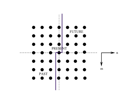
Figure 1: Non-symmetric half plane

Further analysis of the prediction problem led to a generalization of the Wold decomposition [7]. When we consider random processes indexed by a group we obtain a Wold decomposition with respect to any given total order on the group. When the group is not $\mathbb{Z}$ (like $\mathbb{R}$ or $\mathbb{Z}^{2}$) the deterministic process can have as a direct summand a deterministic process of a special type, the evanescent process. In order to provide some intuition on the characteristics of the evanescent process we next state some basic definitions and present an example of an evanescent field defined with respect to a vertical total order, which is simply a lexicographic order on $\mathbb{Z}^{2}$:

A homogeneous random field $\{y(n,m)\}$ is called regular with respect to the lexicographic order if for every $(n,m)$, $E[y(n,m)-\hat{y}(n,m)]^{2}=\sigma^{2}>0$ where $\hat{y}(n,m)$ is the projection of $y(n,m)$ on the $c.l.m.\,\Big{[}\{y(k,l):\,k<n,l\in\mathbb{Z}\}\cup\{y(n,l):\,l<m\}\Big{]}$, where $c.l.m.$ denote a closed linear manifold. Thus, a regular homogeneous random field has a non-zero innovation at every lattice point. A homogeneous random field $\{z(n,m)\}$ is called deterministic with respect to the lexicographic order if it can be perfectly linearly predicted from its past in mean-square sense, i.e., for every $(n,m)$ we have $z(n,m)\in c.l.m.\,\Big{[}{\{z(k,l):\,k<n,l\in\mathbb{Z}\}}\cup\{z(n,l):\,l<m\}\Big{]}$.

Although a deterministic field can be perfectly predicted from its past with respect to lexicographic order, it may still posses a non-zero innovation when prediction is based on samples in previous columns only. We then say that the field $\{z(n,m)\}$ has vertical column-to-column innovations if $I(n,m):=z(n,m)-\hat{z}(n,m)$ (the innovation) is not 0, where $\hat{z}(n,m)$ is the orthogonal projection of $z(n,m)$ on the closed subspace generated by $\{z(k,l):\,k<n,l\in\mathbb{Z}\}$. In other words, if a deterministic field has non-zero column-to-column innovations it cannot be perfectly linearly predicted from previous columns.

When $z(n,m)$ is the deterministic component of the decomposition of a regular random field with respect to a NSHP total-ordering, the vertical evanescent component $z_{e}(n,m)$ is the orthogonal projection of $z(n,m)$ on the closed subspace generated by the (orthogonal) column-to-column innovations $\{I(k,l):\,k\leq n,l\in\mathbb{Z}\}$. Thus, an evanescent field spans a Hilbert space identical to the one spanned by column-to-column innovations. In other words, the evanescent field is a component of the deterministic field which represents column-to-column innovations. Horizontal column-to-column (row-to-row) innovations and evanescent components are similarly defined.

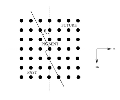
Figure 2: RNSHP support.

Evanescent processes were first introduced in [7] (on ${\mathbb{R}}$). In Korezlioglu and Loubaton [11], “horizontal” and “vertical” total-orders and the corresponding horizontally and vertically evanescent components of a homogeneous random field on ${\mathbb{Z}}^{2}$ are defined. In Kallianpur [9], as well as in Chiang [1], similar techniques are employed to obtain four-fold orthogonal decompositions of regular (non-deterministic) homogeneous random fields. In Francos et. al. [2] this decomposition of random fields on ${\mathbb{Z}}^{2}$ was further extended. This is done by considering all the Rational Non-Symmetrical Half Plane (RNSHP) linear orders, each inducing a different partitioning of the two-dimensional lattice into two sets by a broken straight line of rational slope. Intuitively, the usual lexicographic order is not the only possible order definition of the 2-D lattice. Each RNSHP linear order is induced by a “rotation” of the usual lexicographic order, such that the resulting non-symmetrical half-plane is delimited by a broken straight line with rational slope, and which leads to a different linear order definition. Consequently, terms such as “past” and “future” are redefined with respect to a specific RNSHP linear order (see, for example, Figure 2).

More specifically, each Rational Non Symmetrical Half Plane is defined in terms of two co-prime integers $(a,b)$, such that the past $P_{a,b}$ is defined by

$$P_{a,b}=\{(n,m)\in\mathbb{Z}^{2}:na+mb<0\ \mbox{, or}\ na+mb=0\ \mbox{and}\ m\leq 0\}.$$ (1)

Then $P=P_{a,b}$ satisfies

$$(i)\ P\cap(-P)=\{0\},\quad(ii)\ P\cup(-P)=\mathbb{Z}^{2},\quad(iii)\ P+P\subset P\ (usual\ addition).$$

By (i)-(iii), $P$ induces on $\mathbb{Z}^{2}$ a linear order, which is defined by $(k,l)\preceq(n,m)$ if and only if $(k-n,l-m)\in P$.

Clearly, there are countably many such linear orders. Each such order induces a different definition of the term “column”, and correspondingly different definitions of column-to-column innovations and evanescent field.

The Wold decomposition of a regular random field into purely-indeterministic and deterministic components is invariant to the choice of a RNSHP order. The decomposition in [2] further asserts that we can represent the deterministic component of the field as a mutually orthogonal sum of a “half-plane deterministic” field and a countable number of evanescent fields. The half-plane deterministic field has no innovations, nor column-to-column innovations, with respect to any RNSHP linear order. On the other hand, each of the evanescent fields can be revealed only by using the corresponding RNSHP linear order, i.e., with respect to specific definitions of “columns” and column-to-column innovations. This decomposition yields a corresponding spectral decomposition, i.e., we can decompose the spectral measure of the deterministic part into a countable sum of mutually singular spectral measures, such that the spectral measure of each evanescent component is concentrated on a line with a rational slope.

Based on these results, a parametric model of the homogeneous random field was derived in [2]. The purely-indeterministic component of the field is modeled by a white innovations driven 2-D moving average process with respect to some RNSHP linear order. This component contributes the absolutely continuous part of the spectral measure of the regular field. One of the components of the half-plane deterministic component that is often found in practical applications is the 2-D harmonic random field which is the sum of a countable number of exponential components, each having a constant spatial frequency and random amplitude. This component contributes the 2-D delta functions in the spectral domain. The number of evanescent components of the regular field is countable. The model of the evanescent field with respect to specific order is presented bellow:

Let $(a,b)$ be a pair of co-prime integers ($a\geq 0$) which defines a specific RNSHP linear order according to (1). Then, the model of the evanescent field which corresponds to this order is

$$e_{(a,b)}(n,m)=\sum_{i=1}^{I_{(a,b)}}s_{i}^{(a,b)}(na+mb)\exp\biggl{(}{j{\omega^{(a,b)}_{i}}(nc+md)}\biggr{)}\ ,$$ (2)

where $c$ and $d$ are co-prime integers satisfying $ad-bc=1$. For the case where $(a,b)=(0,1)$ we have $(c,d)=(1,0)$, and for $(a,b)=(1,0)$ we have $(c,d)=(0,1)$. We further note that in this notation $na+mb$ is the “column” index and $nc+md$ defines a “row”. The modulating process $\{s_{i}^{(a,b)}(na+mb)\}$ is a 1-D purely-indeterministic, complex valued processes, and $\omega^{(a,b)}_{i}$ is a modulation frequency. Thus, $e_{(a,b)}$ has no innovations, with respect to “rows”, and has non-zero column-to-column innovation (expressed by the modulating process $s_{i}^{(a,b)}$) with respect to its “columns”. $I_{(a,b)}$ denotes the number of different evanescent components that correspond to the same RNSHP defined by $(a,b)$. The different components are such that their 1-D modulating processes $\{s_{i}^{(a,b)}\}$ and $\{s_{j}^{(a,b)}\}$, are mutually orthogonal and their modulation frequencies are different $\omega^{(a,b)}_{i}\neq\omega^{(a,b)}_{j}$ for all $1\leq i\neq j\leq I_{(a,b)}$.

The “spectral density function” of each evanescent field has the form of a sum of 1-D delta functions which are supported on lines of rational slope in the 2-D spectral domain. The amplitude of each of these delta functions is determined by the spectral density of the 1-D modulating process. Since the spectral density of the modulating process can rapidly decay to zero, so will the “spectral density” of the evanescent field, and hence the name “evanescent”.

1.2 Practical Applications

Besides its fundamental theoretical importance, the Wold decomposition of a regular random field has various applications in image processing and wave propagation problems. For example, the parametric model that results from these orthogonal decompositions, naturally arises as the physical model in problems of texture modeling, estimation and synthesis [3].

Another application is space-time adaptive processing of airborne radar data [4]. Space-time adaptive processing (STAP) is an increasingly popular radar signal processing technique for detecting slow-moving targets. The space dimension arises from the use of array of multiple antenna elements and the time dimension arises from the use of coherent train of radar pulses. The power of STAP comes from the joint processing along the space and time dimensions. Comprehensive analysis of STAP appears in [10, 12].

In [4] it is shown that the same parametric model that results from the 2-D Wold-like orthogonal decomposition naturally arises as the physical model in the problem of space-time processing of airborne radar data. This correspondence is exploited to derive computationally efficient detection algorithms. More specifically, the target signal is modeled as a random amplitude complex exponential where the exponential is defined by a space-time steering vector that has the target’s angle and Doppler. Thus, in the space-time domain the target contribution is the half-plan deterministic component of the observed field. The sum of the white noise field due to the internally generated receiver amplifier noise, and the sky noise contribution, is the purely-indeterministic component of the space-time field decomposition.

The presence of a jammer (a foe interference source, transmitting high power noise aimed at “blinding” the radar system) results in a barrage of noise localized in angle and uniformly distributed over all Doppler frequencies (since the transmitted noise is white). Hence, in the space-time domain each jammer is modeled as an evanescent component with $(a,b)=(0,1)$ such that its 1-D modulating process $s_{i}^{(0,1)}(m)$ is the random process of the jammer amplitudes. The jammer samples from different pulses are uncorrelated. In the angle-Doppler domain each jammer contributes a 1-D delta function, parallel to the Doppler axis and located at a specific angle $\omega_{i}^{(0,1)}$ using the notation of (2).

The ground clutter results in an additional evanescent component of the observed 2-D space-time field. The aircraft platform motion produces a very special structure of the clutter due to the dependence of the Doppler frequency on angle. The clutter’s echo from a single ground patch has a Doppler frequency that linearly depends on its aspect with respect to the platform. As the platform moves, identical clutter observations are repeated by different antenna elements on different pulses, which defines a specific linear locus in the angle-Doppler domain, commonly referred as the “clutter ridge”. Thus, the clutter ridge, which represents clutter from all angles, is supported on a diagonal line (that generally wraps around) in the angle-Doppler domain. Due to the physical properties of the problem the different components of the field are assumed to be mutually orthogonal. In the specific application of airborne radar, the evanescent components (the clutter, and jamming signals) are considered unknown interferences.

Although the data collected by STAP radars for different ranges can be viewed as a sequence of finite-sample realizations from a homogenous field, its is technically more convenient to represent each of the observations in a vector form and to statistically analyze them as multivariate vectors. Thus, if one uses a STAP system with $N$ antenna elements and $M$ pulses, the observed $N\times M$ STAP signal is treated as $NM\times 1$ multivariate random variable. These vectors are commonly called “snapshots”.

The STAP processor goal is to solve a detection problem, i.e., to establish whether a hypothetical target is present or not. It adaptively weights the available data in order to achieve high gain at the target’s angle and Doppler and maximal mitigation along both the jamming and clutter lines. The adaptive weight vector is computed from the inverse of the interference-plus-noise covariance matrix,[10, 12]. It is shown in [5] that the dominant eigenvectors of the space-time covariance matrix contain all the information required to mitigate the interference. Thus, the weight vector is constrained to be in the subspace orthogonal to the dominant eigenvectors. Because the interference-plus-noise covariance matrix is unknown a priori, it is typically estimated using sample covariances obtained from averaging over a few range gates. This is the known as the fully adaptive STAP approach. The major drawback of this approach is its high computational complexity. The final detection of a target is performed by applying either Constant-False-Alarm-Rate (CFAR) detector, or Adaptive-Matched-Filter (AMF) detector, or Generalized-Likelihood-Ratio (GLR) detector. Usually the detector is embedded into the weight computations.

Fortunately, both the clutter and the jammers have low-rank covariance matrices. The clutter covariance matrix has a low rank due to the movement of the platform, as discussed above. The jammer covariance matrix has low rank since the jamming signal is spatially correlated between all antennas at each pulse. The low-rank structure of the interference covariance matrix may be exploited to achieve significant reduction in the adaptive problem dimensionality with little or no sacrifice in performance relative to the fully adaptive case. These methods are referred to as partially adaptive STAP.

Partially adaptive STAP methods require knowledge of the rank of the interference covariance matrix. However, it is a priori unknown, and unfortunately cannot be easily estimated from the sample covariance matrix due to the existence of a noise component which has a full rank covariance matrix. Hence, the problem of estimating the rank of the interference covariance matrix is critical in the implementation of many STAP algorithms.

In this work we consider the problem of determining the rank of the covariance matrix of a vectorized finite dimension sample from an evanescent random field. By using the evanescent field parametric model to model the interferences in the STAP problem, we considerably simplify the solution to the problem of estimating the rank of the low-rank interference covariance matrix. In fact, it turns out that in this parametric framework the well-known Brennan rule [12] for the rank of the clutter covariance matrix, as well as the rank computation of the jammer, become special cases of the general result proved here. Hence, the provided derivation opens the way for new, computationally attractive, methods in parametric and non-parametric estimation of two-dimensional random fields, with immediate applications in partially adaptive space-time adaptive processing of airborne radar data.

The rest of the paper is organized as follows: In Section 2 we formulate the problem we aim to solve. A formula for the rank of the covariance matrix of a complex valued evanescent random field is derived in Section 3. In Section 4 we extend the obtained result to the case of a real valued evanescent random field. Finally, in Section 5 we provide our conclusions.

The following notation is used throughout. Boldface upper case letters denote matrices, boldface lower case letters denote column vectors, and standard lower case letters denote scalars. The superscripts $(\cdot)^{T}$ and $(\cdot)^{H}$ denote the transpose and Hermitian transpose operators, respectively. By ${\bf I}$ we denote the identity matrix and by ${\bf 0}$ a matrix of zeros. The symbol $\odot$ denotes an element by element product of the vectors (Hadamard product). Given a scalar function $f(\cdot)$ and a column vector ${\bf v}$, we denote by $f({\bf v})$ a column vector consisting of the values of function $f(\cdot)$ evaluated for all the elements of ${\bf v}$. Finally $diag({\bf v})$ denotes a square diagonal matrix with the elements of ${\bf v}$ on its main diagonal.

2 Finite Sample of an Evanescent Random Field: Definitions and Problem Formulation

Let $O$ denote the set of all possible pairs of different co-prime integers $(a,b)$, $a\geq 0$, where each pair defines a RNSHP order on the 2-D lattice. Although in the case of an infinite 2-D lattice the number of different RNSHP definitions is infinitely countable, in the finite sample case only a finite number of different linear orders can be defined. Moreover, in practical applications the number of different evanescent components for each order definition is finite as well. Therefore, we assume throughout this paper that $|O|$ and $I_{(a,b)}$ are finite integers.

Let $Q=\sum_{(a,b)\in O}I_{(a,b)}$. Each of the $Q$ evanescent components is uniquely defined by the triple $(a,b,\omega^{(a,b)}_{i})$ where $(a,b)\in O$ and $\omega^{(a,b)}_{i}$ is the frequency parameter. Let us denote the set of all possible triples by $O_{Q}=\{(a_{1},b_{1},\omega_{1}),(a_{2},b_{2},\omega_{2}),\ldots,(a_{Q},b_{Q},\omega_{Q})\}$. All triples are unique: they either have different support parameters $(a_{i},b_{i})\neq(a_{j},b_{j})$, or in case $(a_{i},b_{i})=(a_{j},b_{j})$ they have different frequencies such that $\omega_{i}\neq\omega_{j}$.

Finally, adapting (2) to the finite sample case we have that

$$e(n,m)=\sum_{q=1}^{Q}e_{q}(n,m),$$ (3)

where

$$e_{q}(n,m)=s_{q}(na_{q}+mb_{q})\exp\biggl{(}{j{\omega_{q}}(nc_{q}+md_{q})}\biggr{)}$$ (4)

such that $(a_{q},b_{q},\omega_{q})\in O_{Q}$ and $\{s_{q}\},c_{q},d_{q}$ are defined as above.

We note that since the spectral measure of $\{e_{q}(n,m)\}$ is concentrated on a line (that may wrap around) whose slope is determined by $a_{q}$ and $b_{q}$, we interchangeably refer to $a_{q}$ and $b_{q}$ as either the spectral support parameters of $\{e_{q}\}$ or as the RNSHP slope parameters.

Let $\{e(n,m):(n,m)\in D\}$ where $D=\{(n,m)\in\mathbb{Z}^{2}:0\leq n\leq N-1,\,0\leq m\leq M-1\}$ be the observed finite sample of the random field (3). Let ${\bf e}$ denote an $NM\times 1$ vector form representation of this finite sample:

$${\bf e} = \left[e(0,0),\dots,e(0,M-1),e(1,0),\dots,e(1,M-1),\dots,\right.$$ (5)

$$\left.\dots,e(N-1,0),\dots,e(N-1,M-1)\right]^{T}.$$

This is a multivariate representation of a finite sample of an evanescent random field.

Let $\Gamma$ denote the $NM\times NM$ covariance matrix of the evanescent vector ${\bf e}$,

$${\mbox{\boldmath$\Gamma$}}=E\bigg{[}{\bf e}\left({\bf e}\right)^{H}\bigg{]}.$$ (6)

Due to the special structure of the evanescent field, many of the elements of ${\bf e}$ are linearly dependent, and therefore $\Gamma$ is low-rank. This property is easily demonstrated by considering a single evanescent component that corresponds to the vertical order $(a,b)=(0,1)$ (single jammer source using the STAP nomenclature), with some arbitrary modulation frequency $\omega$ and modulating process $s(m)$. In that case

$$e^{(0,1)}(n,m)=s(m)\exp\biggl{(}{j{\omega}n}\biggr{)}$$ (7)

The vector form representation of the finite sample of this evanescent field is

$${\bf e}^{(0,1)} = \left[s(0),s(1),\dots,s(M-1),s(0)\exp({j{\omega}}),\dots,s(M-1)\exp({j{\omega}}),\dots\right.$$ (8)

$$\left.s(0)\exp({j{\omega}(N-1)})\dots,s(M-1)\exp({j{\omega}(N-1)})\right]^{T}.$$

Since the modulating frequency $\omega$ is a deterministic constant, it is obvious that ${\bf e}^{(0,1)}$ is comprised of only $M$ independent random variables. Therefore, the rank of ${\mbox{\boldmath$\Gamma$}}^{(0,1)}=E\bigg{[}{\bf e}^{(0,1)}\left({\bf e}^{(0,1)}\right)^{H}\bigg{]}$ is also $M$.

The aim of this paper is to derive an expression for the rank of the low-rank covariance matrix $\Gamma$ of the evanescent vector ${\bf e}$, in the general case (3).

3 The Rank of the Covariance Matrix of an Evanescent Field

In this section we derive an expression for the rank of the covariance matrix $\Gamma$. In order to do so, we have to find and quantify the linear dependencies between the samples of ${\bf e}$. Unfortunately, for arbitrary spectral support parameters and multiple evanescent components, this task involves tedious calculations. The results of the entire analysis in this section can be summarized by the following theorem:

Theorem 1.

Let ${\bf e}$ be a vector-form representation of a finite sample from a sum of evanescent random fields, given by (3)-(5). Then, the rank of its covariance matrix, $\Gamma$, is given by

$$rank({\mbox{\boldmath$\Gamma$}})=\min\left(NM,\biggl{[}N\sum_{q=1}^{Q}|a_{q}|+M\sum_{q=1}^{Q}|b_{q}|-\sum_{q=1}^{Q}|a_{q}|\sum_{q=1}^{Q}|b_{q}|\biggr{]}\right).$$ (9)

Even though the evaluations in the next subsections are technical in nature, the obtained result is surprisingly interesting. Hence, before addressing the proof itself let us make some comments. From Theorem 1, it is clear that the rank of the covariance matrix of a finite sample from an evanescent random field is completely determined by the spectral support parameters $(a_{q},b_{q})$ of the different evanescent components, while it is independent of the other parameters of the evanescent fields, such as the parameters of the modulating processes, $\{s_{q}\}$, or the modulation frequencies, $\omega_{q}$.

Moreover, one can easily observe that the well-known Brennan rule for the rank of the low-rank clutter covariance matrix in the STAP framework, [12] as well as the rank of the covariance matrix of the jamming signals are special cases of this theorem. The Brennan rule states that the rank of the clutter covariance ${\mbox{\boldmath$\Gamma$}}_{clut}$ is given by:

$$rank({\mbox{\boldmath$\Gamma$}}_{clut})=\lfloor N+M\beta-\beta\rfloor$$ (10)

where $\beta$ is the slope of the clutter ridge orientation in the angle-Doppler domain, and $\lfloor\rfloor$ denotes rounding to the nearest integer. It is easy to see that this formula is a special case of the above theorem when only a single evanescent field is observed, and its spectral support parameters are $(a,b)=(1,\beta)$. The rank of the jamming covariance matrix is, [12]:

$$rank({\mbox{\boldmath$\Gamma$}}_{jam})=MJ$$ (11)

where $J$ is a number of sources. Since the spectral support of a single jammer in the angle-Doppler domain is a line parallel to the Doppler axis, and since all jammers are mutually orthogonal, they can be modeled as $J$ vertical evanescent components with spectral support parameters $(a,b)=(0,1)$, such that the rank of the covariance matrix of each individual jammer is $M$ as in the above example.

3.1 Rank derivations

In this subsection we prove Theorem 1. The derivation provides an insight into the structure of the covariance matrix, and explains the nature of its low-rank. Moreover, we explicitly show how columns of the covariance matrix that can be represented as linear combinations of other columns are formed, which yields its low-rank.

Rewriting (3) in a vector form we have ${\bf e}=\sum_{q=1}^{Q}{\bf e}_{q}$, where

$${\bf e}_{q} = \left[e_{q}(0,0),\dots,e_{q}(0,M-1),e_{q}(1,0),\dots,e_{q}(1,M-1),\right.$$ (12)

$$\left.\dots,e_{q}(N-1,0),\dots,e_{q}(N-1,M-1)\right]^{T}.$$

Let

$${\mbox{\boldmath$\xi$}}_{q}=\left[s_{q}(0),s_{q}(b_{q}),\dots,s_{q}((M-1)b_{q}),s_{q}(a_{q}),s_{q}(a_{q}+b_{q}),\dots,s_{q}(a_{q}+(M-1)b_{q}),\right.$$

$$\left.\dots,s_{q}((N-1)a_{q}),s_{q}((N-1)a_{q}+b_{q}),\dots,s_{q}((N-1)a_{q}+(M-1)b_{q})\right]^{T}$$ (13)

be the vector whose elements are the observed samples from the 1-D modulating process $\{s_{q}\}$. Define

$${\bf v}_{q} = \left[\ 0,\ d_{q},\dots,\ (M-1)d_{q},\ c_{q},\ c_{q}+d_{q},\dots,\ c_{q}+(M-1)d_{q},\dots,\right.$$ (14)

$$\left.(N-1)c_{q},\ (N-1)c_{q}+d_{q},\ \dots,\ (N-1)c_{q}+(M-1)d_{q}\ \right]^{T}.$$

Let

$${\bf D}_{q}=diag\biggl{(}\exp(-j{\omega_{q}}{\bf v}_{q})\biggr{)}.$$ (15)

be an $NM\times NM$ diagonal matrix. Thus, using (4), we have that

$${\bf e}_{q}={\bf D}_{q}^{H}{\mbox{\boldmath$\xi$}}_{q}\ .$$ (16)

Let ${\bf s}_{q}$ be a $(N-1)|a_{q}|+(M-1)|b_{q}|+1$ dimensional column vector of consecutive samples of the 1-D modulating process $\{s_{q}\}$. For the case in which $a_{q}>0$ and $b_{q}<0$, ${\bf s}_{q}$ is defined as

$${\bf s}_{q} = \left[s_{q}((M-1)b_{q}),\dots,\dots,s_{q}((N-1)a_{q})\right]^{T}\ ,$$ (17)

while for the case in which $a_{q}\geq 0$ and $b_{q}\geq 0$, ${\bf s}_{q}$ is defined as

$${\bf s}_{q} = \left[s_{q}(0),\dots,\dots,s_{q}((N-1)a_{q}+(M-1)b_{q})\right]^{T}\ .$$ (18)

Thus for any $(a_{q},b_{q})$ we have that

$${\mbox{\boldmath$\xi$}}_{q}={\bf A}_{q}^{T}{\bf s}_{q}$$ (19)

and

$${\bf e}_{q}={\bf D}_{q}^{H}{\bf A}_{q}^{T}{\bf s}_{q},$$ (20)

where ${\bf A}_{q}$ is a real-valued $[(N-1)|a_{q}|+(M-1)|b_{q}|+1]\times NM$ rectangular matrix where each of its columns has a single element whose value is “1”, while all the others are zero. Thus, each column of ${\bf A}_{q}$ “chooses” the single element from the vector ${\bf s}_{q}$ that contributes to the corresponding element of the vector ${\mbox{\boldmath$\xi$}}_{q}$ . Due to boundary effects, resulting from the finiteness of the observation, not all of the elements of the vector ${\bf s}_{q}$ contribute to the vector ${\mbox{\boldmath$\xi$}}_{q}$, unless $|a_{q}|\leq 1$ or $|b_{q}|\leq 1$. Hence some rows of the matrix ${\bf A}_{q}$ may contain only zeros. On the other hand, whenever $na_{q}+mb_{q}=ka_{q}+\ell b_{q}$ for some integers $n,m,k,\ell$ such that $0\leq n,k\leq N-1$ and $0\leq m,\ell\leq M-1$, the same sample from the modulating process $\{s_{q}\}$ is duplicated in the elements of ${\mbox{\boldmath$\xi$}}_{q}$. Therefore, the number of distinct columns in ${\bf A}_{q}$ is equal to the number of elements of ${\bf s}_{q}$ that appear in ${\mbox{\boldmath$\xi$}}_{q}$, i.e., the number of distinct samples from the random process $\{s_{q}\}$ that are found in an observed finite sample of an evanescent field of dimensions $N\times M$. The matrix ${\bf A}_{q}$ depends only on $(a_{q},b_{q})$ and is independent of the modulation frequency $\omega_{q}$ or the modulating process $\{s_{q}\}$.

The rank of covariance matrix $\Gamma$ is strongly related to the number of distinct samples from the random processes $\{s_{q}\}$ for all $1\leq q\leq Q$ which can be found in the evanescent vector ${\bf e}$. Therefore, the rank of $\Gamma$ is tightly related to the ranks of the matrices ${\bf A}_{q}$, $1\leq q\leq Q$.

Let ${{\bf R}_{q}}$ be the covariance matrix of the vector ${\bf s}_{q}$ i.e.,

$${{\bf R}_{q}}=E\bigg{[}{\bf s}_{q}\left({\bf s}_{q}\right)^{H}\bigg{]}.$$ (21)

The matrix ${\bf R}_{q}$ is full rank positive definite since the process $\{s_{q}\}$ is purely-indeterministic. Since the evanescent components $\{e_{q}\}$ are mutually orthogonal we conclude that $\Gamma$, the covariance matrix of ${\bf e}$, has the form

$${\mbox{\boldmath$\Gamma$}}=E\bigg{[}{\bf e}\left({\bf e}\right)^{H}\bigg{]}=\sum_{q=1}^{Q}{\mbox{\boldmath$\Gamma$}}_{q}\ ,$$ (22)

where ${\mbox{\boldmath$\Gamma$}}_{q}$ is the covariance matrix of ${\bf e}_{q}$. Using (20) and (21) we find that

$${\mbox{\boldmath$\Gamma$}}_{q} = E\bigg{[}{\bf e}_{q}\left({\bf e}_{q}\right)^{H}\bigg{]}={\bf D}_{q}^{H}{\bf A}_{q}^{T}{\bf R}_{q}{\bf A}_{q}{\bf D}_{q}\ \ .$$ (23)

Finally,

$${\mbox{\boldmath$\Gamma$}}=\sum_{q=1}^{Q}{\bf D}_{q}^{H}{\bf A}_{q}^{T}{\bf R}_{q}{\bf A}_{q}{\bf D}_{q}\ .$$ (24)

One can rewrite the above expression in a block-matrix form

$${\mbox{\boldmath$\Gamma$}}={\bf C}_{Q}^{H}{\bf R}{\bf C}_{Q}$$ (25)

where

$${\bf C}_{Q}=\bigl{[}{\bf D}_{1}^{H}{\bf A}_{1}^{T}\ldots{\bf D}_{Q}^{H}{\bf A}_{Q}^{T}\bigr{]}^{H},$$ (26)

and

$${\bf R}=diag\bigl{(}\bigl{[}{\bf R}_{1}\dots\bf R_{Q}\bigr{]}\bigr{)}.$$ (27)

is a block-diagonal matrix with the matrices ${\bf R}_{q}$, $1\leq q\leq Q$ on its diagonal, and zeros elsewhere.

Since the covariance matrices ${\bf R}_{q}$ are full rank positive definite, the block-diagonal matrix ${\bf R}$ is full rank positive definite as well. Hence by observation 7.1.6 [8] we have

$$rank({\mbox{\boldmath$\Gamma$}})=rank\left({\bf C}_{Q}\right).$$ (28)

The matrix ${\bf C}_{Q}$ has exactly $NM$ columns, such that each one of its columns corresponds to an entry in the evanescent vector ${\bf e}$, or similarly, each one of its columns corresponds to a point on the original $N\times M$ lattice $D=\{(n,m)\in\mathbb{Z}^{2}:0\leq n\leq N-1,\,0\leq m\leq M-1\}$. More specifically, the $n(M-1)+m$ column of ${\bf C}_{Q}$ corresponds to the $n(M-1)+m$ element of ${\bf e}$ which represents the evanescent field sample at the $(n,m)$ lattice point. (Note that we enumerate the columns starting from zero). In the following we will adopt the abbreviation $[n,m]$ for indexing the $n(M-1)+m$ column of a matrix.

To gain more understanding on the structure of ${\bf C}_{Q}$ let us examine the different matrices ${\bf C}_{Q}$ is comprised of. We begin with ${\bf A}_{q}$ for some $1\leq q\leq Q$: By construction (see (20) and the following explanation) all columns of ${\bf A}_{q}$ are unit vectors, where the single “1” entry in each column chooses the single element from the vector ${\bf s}_{q}$ that contributes to $e(n,m)$ - the evanescent field sample at $(n,m)$ . The single non-zero entry in the $[n,m]$ column of ${\bf A}_{q}$ is located in the $k$’th row where $na_{q}+mb_{q}=k$ (we allow negative indexed rows in the case where $b_{q}<0$). For example if $a_{q}>0$ and $b_{q}>0$, the matrix ${\bf A}_{q}$ is given by

$$\begin{array}[]{c}\\ 0\\ \\ k\\ \\ (N-1)a_{q}+(M-1)b_{q}\end{array}\begin{array}[]{c}\begin{array}[]{ccccc}[0,0]&\cdots&[n,m]&\cdots&[N-1,M-1]\end{array}\\ \begin{bmatrix}1&\cdots&\cdots&0&\cdots&\cdots&\cdots&0&\\ \vdots&&&\vdots&&&&\vdots&\\ \vdots&&&1&&&&\vdots&\\ \vdots&&&\vdots&&&&\vdots&\\ 0&\cdots&\cdots&0&\cdots&\cdots&\cdots&1&\\ \end{bmatrix}\\ \end{array}$$ (29)

Let $(n^{*},m^{*})$ be a solution to the linear Diophantine equation $na_{q}+mb_{q}=k$. Then, the equation is also satisfied by $n=n^{*}+tb_{q}$ and $m=m^{*}-ta_{q}$, where $t$ is an arbitrary integer. Since $(a_{q},b_{q})$ are coprime integers these are the only possible solutions. It means that as soon as $(n+tb_{q},m-ta_{q})\in D$, the corresponding $[n+tb_{q},m-ta_{q}]$ column of ${\bf A}_{q}$ will be equal to its $[n,m]$ column. To find the rank of ${\bf A}_{q}$ we have to evaluate the number of linearly independent columns, i.e., the number of distinct elements of $s_{q}(na_{q}+mb_{q})$ $(n,m)\in D$ which contribute to ${\bf e}$.

Since ${\bf D}_{q}$ is a diagonal matrix, the structure of ${\bf A}_{q}{\bf D}_{q}$ is similar to the structure of ${\bf A}_{q}$ with the only difference being that instead “1” in each column, we have the appropriate exponential coefficient. Therefore, each column of the matrix ${\bf C}_{Q}$ has exactly $Q$ non-zero elements.

Next, let us concatenate the matrices ${\bf A}_{p}$ and ${\bf A}_{q}$, where $1\leq p\neq q\leq Q$ and examine the structure of resulting matrix

$$\tilde{\bf C}_{pq}=[{\bf A}_{p}^{T}\ {\bf A}_{q}^{T}\ ]^{T}.$$ (30)

As before, let us consider the structure of some arbitrary $[n,m]$ column of this matrix. It has two non-zero entries: On the $k_{p}$ row of ${\bf A}_{p}$ and on the $k_{q}$ row of ${\bf A}_{q}$, where $(n,m)$ satisfies

$$na_{p}+mb_{p}=k_{p},$$ (31)

and

$$na_{q}+mb_{q}=k_{q}.$$ (32)

Next, we note that the pair $(n+tb_{p},m-ta_{p})$ satisfies the linear Diophantine equation (31) for any integer $t$. Therefore, for $t_{p}$ such that $(n+t_{p}b_{p},m-t_{p}a_{p})\in D$, the $[n+t_{p}b_{p},m-t_{p}a_{p}]$ column of ${\bf A}_{p}$ has a “1” entry, at the same row as the $[n,m]$ column. However, $(n+t_{p}b_{p},m-t_{p}a_{p})$ also satisfies the linear Diophantine equation

$$(n+t_{p}b_{p})a_{q}+(m-t_{p}a_{p})b_{q}=\ell_{q}.$$ (33)

Hence, the $[n+t_{p}b_{p},m-t_{p}a_{p}]$ column of ${\bf A}_{q}$ has a “1” entry on its $\ell_{q}$ row.

Similarly, since $(n+tb_{q},m-ta_{q})$ satisfies the linear Diophantine equation (32) for any integer $t$, for $t_{q}$ such that $(n+t_{q}b_{q},m-t_{q}a_{q})\in D$ we have that the $[n+t_{q}b_{q},m-t_{q}a_{q}]$ column of ${\bf A}_{q}$ has “1” at the same row as the $[n,m]$ column. Since,

$$(n+t_{q}b_{q})a_{p}+(m-t_{q}a_{q})b_{p}=\ell_{p},$$ (34)

the $[n+t_{q}b_{q},m-t_{q}a_{q}]$ column of ${\bf A}_{p}$ has “1” on its $\ell_{p}$ row. Moreover, one can observe that for a pair of integers $(t_{p},t_{q})$ such that $(n+t_{p}b_{p}+t_{q}b_{q},m-t_{p}a_{p}-t_{q}a_{q})\in D$, the pair $(n+t_{p}b_{p}+t_{q}b_{q},m-t_{p}a_{p}-t_{q}a_{q})$ simultaneously satisfies (33) and (34):

$$(n+t_{p}b_{p}+t_{q}b_{q})a_{p}+(m-t_{p}a_{p}-t_{q}a_{q})b_{p} = \ell_{p}$$

$$(n+t_{p}b_{p}+t_{q}b_{q})a_{q}+(m-t_{p}a_{p}-t_{q}a_{q})b_{q} = \ell_{q}$$ (35)

Therefore the $[n+t_{p}b_{p}+t_{q}b_{q},m-t_{p}a_{p}-t_{q}a_{q}]$ column of of ${\bf A}_{p}$ has “1” on its $\ell_{p}$ row, and the same column of ${\bf A}_{q}$ has “1” on its $\ell_{q}$ row.

Finally, we can represent the $[n,m]$ column of $\tilde{\bf C}_{pq}$ by a linear combination of its other columns:

$$[n,m] = [n+t_{p}b_{p},m-t_{p}a_{p}]+[n+t_{q}b_{q},m-t_{q}a_{q}]-$$ (36)

$$[n+t_{p}b_{p}+t_{q}b_{q},m-t_{p}a_{p}-t_{q}a_{q}],$$

or in a more detailed form by

$$\begin{array}[]{c}\\ k_{p}\\ \\ k_{q}\\ \\ \\ \end{array}\left[\begin{array}[]{c}\\ 1\\ \\ 1\\ \\ \\ \end{array}\right]=\begin{array}[]{c}\\ k_{p}\\ \\ \\ \ell_{q}\\ \\ \end{array}\left[\begin{array}[]{c}\\ 1\\ \\ \\ 1\\ \\ \end{array}\right]+\begin{array}[]{c}\\ \\ \ell_{p}\\ k_{q}\\ \\ \\ \end{array}\left[\begin{array}[]{c}\\ \\ 1\\ 1\\ \\ \\ \end{array}\right]-\begin{array}[]{c}\\ \\ \ell_{p}\\ \\ \ell_{q}\\ \\ \end{array}\left[\begin{array}[]{c}\\ \\ 1\\ \\ 1\\ \\ \end{array}\right]$$ (37)

Let $T_{pq}^{(n,m)}$ be the set of all the integer pairs $(t_{p},t_{q})$ such that $(n+t_{p}b_{p},m-t_{p}a_{p}),(n+t_{q}b_{q},m-t_{q}a_{q}),(n+t_{p}b_{p}+t_{q}b_{q},m-t_{p}a_{p}-t_{q}a_{q})\in D$. Clearly, the set $T_{pq}^{(n,m)}$ is non-empty since $(0,0)\in T_{pq}^{(n,m)}$, and it corresponds to a trivial representation of the $[n,m]$ column by itself. If $|T_{pq}^{(n,m)}|>1$ then the $[n,m]$ column has non-trivial linear representation by other columns.

Recall however, that the matrix ${\bf C}_{Q}$ is comprised of blocks where each block is of the form ${\bf A}_{q}{\bf D}_{q}$. Consider next the concatenation of two such blocks ${\bf A}_{p}{\bf D}_{p}$ and ${\bf A}_{q}{\bf D}_{q}$,

$${\bf C}_{pq}=[{\bf D}_{p}^{H}{\bf A}_{p}^{T}\ {\bf D}_{q}^{H}{\bf A}_{q}^{T}\ ]^{H}.$$ (38)

Keeping in mind that by definition $a_{p}d_{p}-b_{p}c_{p}=1$ and $a_{q}d_{q}-b_{q}c_{q}=1$, it is easy to check that the replacement of the “1” in the columns of $\tilde{\bf C}_{pq}$ by exponentials as in (38) will only affect the coefficients of the linear combination. Indeed, the linear combination of columns in this case has the form

$$[n,m] = [n+t_{p}b_{p},m-t_{p}a_{p}]\exp({j\omega_{p}t_{p}})+[n+t_{q}b_{q},m-t_{q}a_{q}]\exp({j\omega_{q}t_{q}})$$ (39)

$$- [n+t_{p}b_{p}+t_{q}b_{q},m-t_{p}a_{p}-t_{q}a_{q}]\exp({j[\omega_{p}t_{p}+\omega_{q}t_{q}]}).$$

One may also notice that if $(a_{p},b_{p})=(a_{q},b_{q})$ we have that $k_{p}=k_{q}=\ell_{p}=\ell_{q}$. However, since in this case $\omega_{p}\neq\omega_{q}$ the linear combination in (39) is still valid and non-trivial.

It is clear that the linear dependencies of columns of ${\bf C}_{Q}$ are governed by the same simple laws: Let $T_{Q}^{(n,m)}$ be a set of all $Q$-tuples of integers $(t_{1},\ldots,t_{Q})$ defined as follows: For any $1\leq q\leq Q$, let $(i_{1},\ldots,i_{q})$ be a set of $q$ indices, such that $1\leq i_{k}\leq Q$ for all $1\leq k\leq q$, and

$$(n+t_{i_{1}}b_{i_{1}}+\ldots+t_{i_{q}}b_{i_{q}},m-t_{i_{1}}a_{i_{1}}-\ldots-t_{i_{q}}a_{i_{q}})\in D.$$

Clearly, the set $T_{Q}^{(n,m)}$ is non-empty since $(0,\ldots,0)\in T_{Q}^{(n,m)}$. Let $(n,m)\in D$ be an arbitrary lattice point and let $[n,m]$ be its corresponding column in ${\bf C}_{Q}$. Then, the $[n,m]$ column can be represented by the linear combination

$$[n,m]=$$

$$\sum_{q=1}^{Q}(-1)^{q-1}\mathop{\underbrace{\sum_{{i_{1}}=1}^{Q-q+1}\ldots\sum_{{i_{q}}={i_{q-1}}+1}^{Q}}}\limits_{\mbox{\emph{q} sums}}[n+t_{i_{1}}b_{i_{1}}+\ldots+t_{i_{q}}b_{i_{q}},m-t_{i_{1}}a_{i_{1}}-\ldots-t_{i_{q}}a_{i_{q}}]\cdot$$

$$\hskip 115.63243pt\cdot\exp\left({j{[\omega_{i_{1}}t_{i_{1}}+\ldots+\omega_{i_{q}}t_{i_{q}}]}}\right),$$ (40)

where $(t_{1},\ldots,t_{Q})\in T_{Q}^{(n,m)}$. The details of this derivation are presented in Appendix A.

Following the foregoing analysis of the linear dependencies between the columns of ${\bf C}_{Q}$, we next count its linearly independent columns in order to derive the rank of ${\bf C}_{Q}$. Let us first count the number of independent columns of ${\bf A}_{q}{\bf D}_{q}$. As mentioned earlier, this number is equal the number of distinct samples from $s_{q}(na_{q}+mb_{q})$, $(n,m)\in D$ that contribute to ${\bf e}$. In other words, this is the number of different indices $k$, such that $na_{q}+mb_{q}=k$ where $(n,m)\in D$, and it can be easily calculated based on the dimensions of $D$ (see Figure 3 for an illustrative example). Indeed, a new sample from the random process $\{s_{q}\}$ may be introduced only on the first $a_{q}$ rows (since $a_{q}\geq 0$) and the last (first) $|b_{q}|$ columns (last if $b_{q}\geq 0$ and first if $b_{q}<0$) of the observed finite dimensional field, while the rest of the field is filled by replicas of these samples. We thus count $Na_{q}$ distinct samples in the first $a_{q}$ rows and $M|b_{q}|$ distinct samples in the first (last) $|b_{q}|$ columns. However, on the intersection of these rows and columns $|a_{q}b_{q}|$ samples are counted twice. Finally, the total number of distinct samples from the random process $\{s_{q}\}$ that are found in an observed field of dimensions $N\times M$ (which is equal to the rank of ${\bf A}_{q}$ and the rank of ${\bf A}_{q}{\bf D}_{q}$) is given by

$$r_{q}=Na_{q}+M|b_{q}|-|a_{q}b_{q}|.$$ (41)

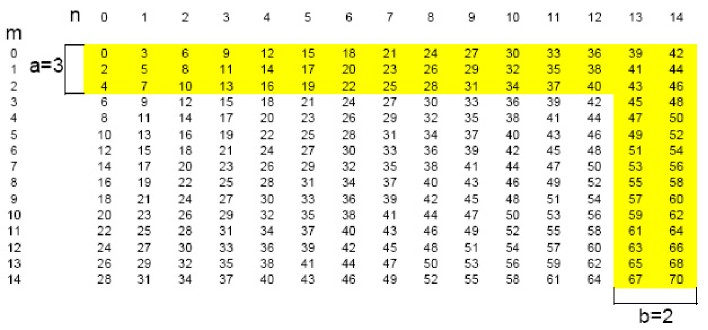
(a)

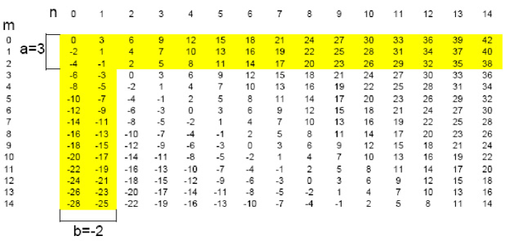
(b)

Figure 3: $N=M=15,a=3,b=\pm 2$: (a) The indices $k=na+mb$ of the observation on $\{s^{(3,2)}(k)\}$; (b) The indices $k=na+mb$ of the observation on $\{s^{(3,-2)}(k)\}$. The sets of distinct indices of $\{s^{(3,2)}(k)\}$ and $\{s^{(3,-2)}(k)\}$ are marked in yellow. Every other sample in the field is identical to some sample in the yellow area.

Similarly, it can be shown that the number of linearly independent columns of ${\bf A}_{p}{\bf D}_{p}$ is $Na_{p}+M|b_{p}|-|a_{p}b_{p}|$. Let us next count the number of linearly independent columns of ${\bf C}_{pq}$.

Since $r_{p}$ columns of ${\bf A}_{p}{\bf D}_{p}$ are linearly independent, the same columns of the concatenated matrix ${\bf C}_{pq}$ are linearly independent as well. The remaining $NM-r_{p}=(N-|b_{p}|)(M-|a_{p}|)$ columns may be considered to correspond to an $(N-|b_{p}|)\times(M-|a_{p}|)$ rectangular sub-lattice $D_{1}=\{(n,m)\in\mathbb{Z}^{2}:0\leq n\leq N-1-|b_{p}|,\,|a_{p}|\leq m\leq M-1\}$ (see Figure 4 as an example), which is a subset of the original rectangular lattice (or similarly, one can define $D_{1}=\{(n,m)\in\mathbb{Z}^{2}:|b_{p}|\leq n\leq N-1,\,|a_{p}|\leq m\leq M-1\}$ which doesn’t change the reasoning of our arguments and only depends on a sign of $b_{p}$). Repeating the same arguments as those made above, one can show that the number of distinct samples from the random process $\{s_{q}\}$ that are found in a sub-lattice $D_{1}$ is

$$\tilde{r_{q}}=(N-|b_{p}|)|a_{q}|+(M-|a_{p}|)|b_{q}|-|a_{q}b_{q}|\ .$$ (42)

This is the number of linearly independent columns which can be found in ${\bf C}_{pq}$ in addition to the first $r_{p}$ columns.

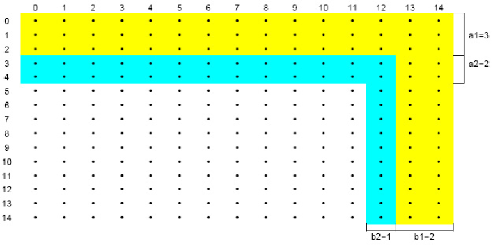
(a)

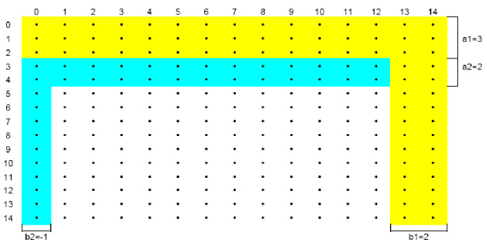
(b)

Figure 4: $N=M=15,a_{1}=3,b_{1}=2,a_{2}=2,b_{2}=\pm 1$. (a): The set of distinct samples of $s^{(3,2)}(n,m)$ (in yellow) and $s^{(2,1)}(n,m)$ (in blue). (b): The set of distinct samples of $s^{(3,2)}(n,m)$ (in yellow) and $s^{(2,-1)}(n,m)$ (in blue). In both cases, every other sample in the field is a linear combination of samples in the colored areas.

Let $D_{2}$ be the set of $NM-r_{p}-\tilde{r}_{q}=(N-|b_{p}|-|b_{p}|)(M-|a_{q}|-|a_{q}|)$ lattice points that remain after the removal from $D$ of the $r_{p}+\tilde{r}_{q}$ points corresponding to the linearly independent columns of ${\bf C}_{pq}$ (for simplicity and without limiting of the generality of the results, we will discuss the case where $b_{p}>0$ and $b_{q}>0$, as illustrated in Figure 2a (uncolored area)). Thus, $D_{2}=\{(n,m)\in\mathbb{Z}^{2}:0\leq n\leq N-1-|b_{p}|-|b_{q}|,\,|a_{p}|+|a_{q}|\leq m\leq M-1\}$. It thus remains to be shown that all columns representing points in $D_{2}$ can be represented by a linear combination of columns that correspond to points in $D\setminus D_{2}$.

Since the “width” of $D\setminus D_{2}$ is $|b_{p}|+|b_{q}|$ along the $n$-axis and $|a_{p}|+|a_{q}|$ along the $m$-axis (colored areas in Figure 4), for every $(n,m)\in D_{2}$ we have $(n+b_{p},m-a_{p}),(n+b_{q},m-a_{q}),(n+b_{p}+b_{q},m-a_{p}-a_{q})\in D$. Thus, $(t_{p},t_{q})=(1,1)\in T_{pq}^{(n,m)}$, and as we have shown above, we can represent $[n,m]$ by the linear combination

$$[n,m] = [n+b_{p},m-a_{p}]\exp({j\omega_{p}})+[n+b_{q},m-a_{q}]\exp({j\omega_{q}})$$ (43)

$$- [n+b_{p}+b_{q},m-a_{p}-a_{q}]\exp({j[\omega_{p}+\omega_{q}]}).$$

Continuing this construction recursively, it is obvious that for each point $(n,m)\in D_{2}$ we can find a pair $(t_{p},t_{q})\in T_{pq}^{(n,m)}$, and $(t_{p},t_{q})\neq(0,0)$ such that $(n+t_{p}b_{p},m-t_{p}a_{p}),(n+t_{q}b_{q},m-t_{q}a_{q}),(n+t_{p}b_{p}+t_{q}b_{q},m-t_{p}a_{p}-t_{q}a_{q})\in D\setminus D_{2}$. On the other hand, for every point $(n,m)\in D\setminus D_{2}$ one can show that $T_{pq}^{(n,m)}=\{(0,0)\}$, i.e., only the trivial linear combination exists. In other words, all the random variables indexed on $D\setminus D_{2}$ correspond to linearly independent columns. Therefore, the number of linearly independent columns in ${\bf C}_{pq}$ is

$$rank(C_{pq})=|D\setminus D_{2}|=r_{p}+\tilde{r_{q}}$$

$$=N(|a_{p}|+|a_{q}|)+M(|b_{p}|+|b_{q}|)-(|a_{p}|+|a_{q}|)(|b_{p}|+|b_{q}|).$$ (44)

The construction described above can be easily extended to the general case where we concatenate all the matrices which ${\bf C}_{Q}$ is comprised of. See Figure 5 for an example of a three component case. If one chooses a subset of the original lattice,

$$D_{Q}=\{(n,m)\in\mathbb{Z}^{2}:0\leq n\leq N-1-\sum_{q=1}^{Q}|b_{q}|,\,\sum_{q=1}^{Q}|a_{q}|\leq m\leq M-1\},$$

which remains after the removal of

$$N\sum_{q=1}^{Q}|a_{q}|+M\sum_{q=1}^{Q}|b_{q}|-\sum_{q=1}^{Q}|a_{q}|\sum_{q=1}^{Q}|b_{q}|$$ (45)

lattice points (similarly to $D_{2}$ which remains after the removal of the $r_{p}+\tilde{r}_{q}$ lattice points corresponding to the independent columns of ${\bf C}_{pq}$), one can repeat the same considerations as above and show that columns of ${\bf C}_{Q}$ that correspond to the lattice points in $D\setminus D_{Q}$ are the only linearly independent columns of ${\bf C}_{Q}$. Thus,

$$rank({\bf C}_{Q})=|D\setminus D_{Q}|=N\sum_{q=1}^{Q}|a_{q}|+M\sum_{q=1}^{Q}|b_{q}|-\sum_{q=1}^{Q}|a_{q}|\sum_{q=1}^{Q}|b_{q}|.$$ (46)

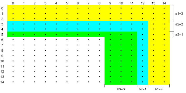
Figure 5: Sets of distinct samples in the case of three evanescent components. $N=M=15,a_{1}=3,b_{1}=2,a_{2}=2,b_{2}=1,a_{3}=1,b_{3}=3$

Finally, Since the rank of $\Gamma$ cannot exceed $NM$ (the dimension of the covariance matrix), $NM$ is an upper bound on the rank of $\Gamma$. Combining this and (46) the rank of $\Gamma$ is given by (9), which completes the proof.

4 The Case of a Real Valued Evanescent Field

In the case where a real valued evanesced field is considered, we have

$$e_{q}(n,m) = s_{q}(na_{q}+mb_{q})\cos({{\omega_{q}}(nc_{q}+md_{q})})$$ (47)

$$+ t_{q}(na_{q}+mb_{q})\sin({{\omega_{q}}(nc_{q}+md_{q})}),$$

where the 1-D purely-indeterministic processes $\{s_{q}\}$, $\{s_{p}\}$, $\{t_{q}\}$, $\{t_{p}\}$ are mutually orthogonal for all $1\leq p\neq q\leq Q$, and for all $q$ the processes $\{s_{q}\}$ and $\{t_{q}\}$ have an identical autocorrelation function. Let ${\bf t}_{q}$ be defined similarly to ${\bf s}_{q}$ in (18). Using similar notations as in (20) we have

$${\bf e}_{q}={\cal R}({\bf D}_{q}^{H}){\bf A}_{q}^{T}{\bf s}_{q}+{\cal I}({\bf D}_{q}^{H}){\bf A}_{q}^{T}{\bf t}_{q},$$ (48)

where ${\cal R}$ and ${\cal I}$ denote real and imaginary parts respectively. Finally, since the processes $\{s_{q}\}$ and $\{t_{q}\}$ are mutually orthogonal and have an identical autocorrelation function we find that

$${\mbox{\boldmath$\Gamma$}}_{q}=E\bigg{[}{\bf e}_{q}\left({\bf e}_{q}\right)^{T}\bigg{]}={\cal R}({\bf D}_{q}^{H}){\bf A}_{q}^{T}{\bf R}_{q}{\bf A}_{q}{\cal R}({\bf D}_{q})+{\cal I}({\bf D}_{q}^{H}){\bf A}_{q}^{T}{\bf R}_{q}{\bf A}_{q}{\cal I}({\bf D}_{q})$$ (49)

where

$${\bf R}_{q}=E\bigg{[}{\bf s}_{q}\left({\bf s}_{q}\right)^{T}\bigg{]}=E\bigg{[}{\bf t}_{q}\left({\bf t}_{q}\right)^{T}\bigg{]}$$ (50)

is positive definite since $\{s_{q}\}$ and $\{t_{q}\}$ are purely-indeterministic.

Similarly to the case of a complex valued evanescent field, the covariance matrix $\Gamma$ is given by

$${\mbox{\boldmath$\Gamma$}}=\sum_{q=1}^{Q}{\mbox{\boldmath$\Gamma$}}_{q}\ .$$ (51)

The derivation of the rank of the covariance matrix (51) follows exactly the same lines as in the previous section, and the next corollary is immediate:

Corollary 1.

Let ${\bf e}$ be a vector-form representation of a finite sample from a sum of real-valued evanescent random fields, given by (3),(47) and (5). Then, the rank of its covariance matrix, $\Gamma$, is given by

$$rank({\mbox{\boldmath$\Gamma$}})=\min\left(NM,\biggl{[}N\sum_{q=1}^{Q}2|a_{q}|+M\sum_{q=1}^{Q}2|b_{q}|-\sum_{q=1}^{Q}2|a_{q}|\sum_{q=1}^{Q}2|b_{q}|\biggr{]}\right).$$ (52)

5 Conclusion

We have considered the problem of evaluating the rank of the covariance matrix of a finite sample from an evanescent random field. We have analytically derived the rank formula and have shown that the rank of the covariance matrix of this finite sample from the evanescent random field is completely determined by the evanescent field spectral support parameters and is independent of all other parameters of the field. Thus, for example, the problem of evaluating the rank of the low-rank covariance matrix of the interference in space time adaptive processing (STAP) of radar data may be solved as a by-product of estimating only the spectral support parameters of the interference components, when we employ a parametric model of the STAP data which is based on Wold decomposition, [4]. Thus , this formula generalizes a well known result known as the Brennan rule for the rank of the clutter covariance matrix in space-time adaptive processing of airborne radar data. The derived rank formula may be employed in a wide range of applications in radar signal processing as well as in other areas of signal and image processing.

6 Appendix A

To derive (40) let us choose an arbitrary lattice point $(n,m)\in D$, and hence a corresponding column $[n,m]$. Exactly as in the two component case, this column is associated with the random variable $e(n,m)$. In fact we are looking for a representation of this random variable by a linear combination of other random variables indexed on $D$.

The first term in the desired linear combination is a sum of $Q$ columns

$$\sum_{i=1}^{Q}[n+t_{i}b_{i},m-t_{i}a_{i}]\exp(j\omega_{i}t_{i}).$$ (53)

This sum creates a new column vector. Similarly to the two component case, this vector is composed of the $Q$ non-zero elements of the $[n,m]$ column (similarly to the elements in rows $k_{p}$ and $k_{q}$ of ${\bf C}_{pq}$), but in addition it includes the undesired elements (similar to the elements in rows $\ell_{p}$ and $\ell_{q}$). The total number of contributed undesired elements is $Q(Q-1)$. Each two pairs $(a_{i},b_{i})$ and $(a_{j},b_{j})$, $i\neq j$, contribute a pair of undesired elements (one in ${\bf A}_{i}{\bf D}_{i}$ and one in ${\bf A}_{j}{\bf D}_{j}$), which can be eliminated by subtraction of the $[n+t_{i}b_{i}+t_{j}b_{j},m-t_{i}a_{i}-t_{j}a_{j}]$ column multiplied by the appropriate exponential coefficient, since

$$(n+t_{i}b_{i})a_{j}+(m-t_{i}a_{i})b_{j}=(n+t_{i}b_{i}+t_{j}b_{j})a_{j}+(m-t_{i}a_{i}-t_{j}a_{j})b_{j}$$

$$(n+t_{j}b_{j})a_{i}+(m-t_{j}a_{j})b_{i}=(n+t_{i}b_{i}+t_{j}b_{j})a_{i}+(m-t_{i}a_{i}-t_{j}a_{j})b_{i}$$ (54)

(See also (35) for the equivalent scenario in the two component case).

To eliminate all these undesired elements we subtract from the vector in (53) the sum of $\binom{Q}{2}$ such columns (half the number of contributed undesired elements), and the result is

$$\sum_{i=1}^{Q}[n+t_{i}b_{i},m-t_{i}a_{i}]\exp({j{\omega_{i}t_{i}}})-$$

$$\sum_{i=1}^{Q-1}\sum_{j=i+1}^{Q}[n+t_{i}b_{i}+t_{j}b_{j},m-t_{i}a_{i}-t_{j}a_{j}]\exp\left({j{[\omega_{i}t_{i}+\omega_{j}t_{j}]}}\right)$$

However, the resulting column now contains a new kind of undesired elements. Substraction of the $[n+t_{i}b_{i}+t_{j}b_{j},m-t_{i}a_{i}-t_{j}a_{j}]$ column has eliminated $2$ undesired elements in ${\bf A}_{i}{\bf D}_{i}$ and ${\bf A}_{j}{\bf D}_{j}$, but at the same time has created a new undesired element in every ${\bf A}_{k}{\bf D}_{k}$, such that $i\neq j\neq k$. A total of $Q-2$ new undesired elements have been created. Clearly, these elements are negative and their total number is $\binom{Q}{2}(Q-2)=3\binom{Q}{3}$. To eliminate the contribution of these elements we add the $[n+t_{i}b_{i}+t_{j}b_{j}+t_{k}b_{k},m-t_{i}a_{i}-t_{j}a_{j}-t_{k}a_{k}]$ column with an appropriate exponential coefficient which eliminates the undesired element from ${\bf A}_{k}{\bf D}_{k}$. At the same time this action is also canceling the undesired result of subtracting $[n+t_{i}b_{i}+t_{k}b_{k},m-t_{i}a_{i}-t_{k}a_{k}]$ that appears in ${\bf A}_{j}{\bf D}_{j}$, and the undesired result of subtracting $[n+t_{j}b_{j}+t_{k}b_{k},m-t_{j}a_{j}-t_{k}a_{k}]$ in ${\bf A}_{i}{\bf D}_{i}$. This is because it can be easy verified that indeed

$$(n+t_{i}b_{i}+t_{j}b_{j})a_{k}+(m-t_{i}a_{i}-t_{j}a_{j})b_{k}=$$

$$\hskip 28.90755pt(n+t_{i}b_{i}+t_{j}b_{j}+t_{k}b_{k})a_{k}+(m-t_{i}a_{i}-t_{j}a_{j}-t_{k}a_{k})b_{k},$$

$$(n+t_{i}b_{i}+t_{k}b_{k})a_{j}+(m-t_{i}a_{i}-t_{k}a_{k})b_{j}=$$

$$\hskip 28.90755pt(n+t_{i}b_{i}+t_{j}b_{j}+t_{k}b_{k})a_{j}+(m-t_{i}a_{i}-t_{j}a_{j}-t_{k}a_{k})b_{j},$$

$$(n+t_{j}b_{j}+t_{k}b_{k})a_{i}+(m-t_{j}a_{j}-t_{k}a_{k})b_{i}=$$

$$\hskip 28.90755pt(n+t_{i}b_{i}+t_{j}b_{j}+t_{k}b_{k})a_{i}+(m-t_{i}a_{i}-t_{j}a_{j}-t_{k}a_{k})b_{i}.$$ (56)

To eliminate all undesired elements we add to the vector in (6), $\binom{Q}{3}$ such columns, and the result is

$$\sum_{i=1}^{Q}[n+t_{i}b_{i},m-t_{i}a_{i}]\exp({j{\omega_{i}t_{i}}})-$$

$$\sum_{i=1}^{Q-1}\sum_{j=i+1}^{Q}[n+t_{i}b_{i}+t_{j}b_{j},m-t_{i}a_{i}-t_{j}a_{j}]\exp\left({j{[\omega_{i}t_{i}+\omega_{j}t_{j}]}}\right)+$$

$$\sum_{i=1}^{Q-2}\sum_{j=i+1}^{Q-1}\sum_{k=j+1}^{Q}[n+t_{i}b_{i}+t_{j}b_{j}+t_{k}b_{k},m-t_{i}a_{i}-t_{j}a_{j}-t_{k}a_{k}]\cdot$$

$$\hskip 79.49744pt\cdot\exp\left({j{[\omega_{i}t_{i}+\omega_{j}t_{j}+\omega_{k}t_{k}]}}\right)$$ (57)

The last action canceled $\binom{Q}{2}(Q-2)=3\binom{Q}{3}$ undesired elements and created once again new $\binom{Q}{3}(Q-3)=4\binom{Q}{4}$ undesired elements. We repeat this procedure $Q$ times and in each step $k$, $1\leq k\leq Q$, we subtract/add $\binom{Q}{k}$ columns for canceling $k\binom{Q}{k}$ undesired elements created in the previous step. Due to this substraction/addition new $\binom{Q}{k}(Q-k)=(k+1)\binom{Q}{k+1}$ undesired elements are created. Clearly, when we subtract/add $\binom{Q}{Q-1}$ columns exactly $Q=Q\binom{Q}{Q}$ undesired elements are created. These may be canceled by substraction of a single vector. By substraction/addition of the last vector, $[n+t_{1}b_{1}+\ldots+t_{Q}b_{Q},m-t_{1}a_{1}-\ldots-t_{Q}a_{Q}]$ the process terminates, since we are canceling the last $Q$ undesired elements and remain with $Q$ elements – exactly those of the $[n,m]$ column, i.e.,

$$[n,m]=\sum_{i=1}^{Q}[n+t_{i}b_{i},m-t_{i}a_{i}]\exp({j{\omega_{i}t_{i}}})-$$

$$\sum_{i=1}^{Q-1}\sum_{j=i+1}^{Q}[n+t_{i}b_{i}+t_{j}b_{j},m-t_{i}a_{i}-t_{j}a_{j}]\exp\left({j{[\omega_{i}t_{i}+\omega_{j}t_{j}]}}\right)+\ldots$$

$$(-1)^{Q-1}[n+t_{1}b_{1}+\ldots+t_{Q}b_{Q},m-t_{1}a_{1}-\ldots-t_{Q}a_{Q}]\exp\left({j{[\omega_{1}t_{1}+\ldots+\omega_{Q}t_{Q}]}}\right)=$$

$$\sum_{q=1}^{Q}(-1)^{q-1}\mathop{\underbrace{\sum_{{i_{1}}=1}^{Q-q+1}\ldots\sum_{{i_{q}}={i_{q-1}}+1}^{Q}}}\limits_{\mbox{\emph{q} sums}}[n+t_{i_{1}}b_{i_{1}}+\ldots+t_{i_{q}}b_{i_{q}},m-t_{i_{1}}a_{i_{1}}-\ldots-t_{i_{q}}a_{i_{q}}]\cdot$$

$$\hskip 108.405pt\cdot\exp\left({j{[\omega_{i_{1}}t_{i_{1}}+\ldots+\omega_{i_{q}}t_{i_{q}}]}}\right)$$ (58)

Clearly, this linear combination will be meaningful only if $(t_{1},\ldots,t_{Q})\in T_{Q}^{(n,m)}$, i.e., $(n+t_{i_{1}}b_{i_{1}}+\ldots+t_{i_{q}}b_{i_{q}},m-t_{i_{1}}a_{i_{1}}-\ldots-t_{i_{q}}a_{i_{q}})\in D,$ for any $1\leq q\leq Q$, and where $(i_{1},\ldots,i_{q})$ is such that $1\leq i_{k}\leq Q$ for all $1\leq k\leq q$.

References

- [1] T. P. Chiang, “The Prediction Theory of Stationary Random Fields III, Fourfold Wold Decompositions,” Jou. Multivariate Anal., vol. 37, pp. 46-65, 1991.
- [2] J. M. Francos, A. Z. Meiri, and B. Porat, “A Wold-like decomposition of 2-D discrete homogenous random fields,” Ann. Appl. Prob., vol. 5, pp. 248-260, 1995.
- [3] J. M. Francos, A. Narashimhan, and J. W. Woods, “Maximum-Likelihood Estimation of Textures Using a Wold Decomposition Model,” IEEE Trans. Image Process., vol. 4, pp. 1655-1666, 1995.
- [4] J. M. Francos and A. Nehorai, “Interference Mitigation in STAP Using the Two-Dimensional Wold Decomposition Model,” IEEE Tran. Signal Proces., vol. 51, pp. 2461-2470, 2003.
- [5] A. Haimovich, “The Eigencanceler: Adaptive radar by eigenanalysis methods,” IEEE Trans. Aeor. Elect. Syst., vol. 32, pp. 532-542, 1996.
- [6] H. Helson and D. Lowdenslager, “Prediction Theory and Fourier Series in Several Variables,” Acta Mathematica., 99, pp. 165-201, 1958.
- [7] H. Helson and D. Lowdenslager, “Prediction Theory and Fourier Series in Several Variables II,” Acta Mathematica, vol. 106, pp. 175-213, 1961.
- [8] R. A. Horn and C. R. Johnson, Topics in Matrix Analysis, Cambridge University Press, 1991.
- [9] G. Kallianpur , A. G. Miamee and H. Niemi, “On the Prediction Theory of Two-Parameter Stationary Random Fields,” Jou. Multivariate Anal., vol. 32, pp. 120-149, 1990.
- [10] R. Klemm, Principles of Space Time Adaptive Processing, IEE Publishing, London, 2002.
- [11] H. Korezlioglu and P. Loubaton, “Spectral Factorization of Wide Sense Stationary Processes on ,” Jou. Multivariate Anal., vol. 19, pp. 24-47, 1986.
- [12] J. Ward, Space-Time Adaptive Processing for Airborne Radar. Technical Report 1015, Lincoln Laboratory, MIT, 1994.
- [13] H. Wold, The Analysis of Stationary Time Series, 2nd ed, Almquist and Wicksell, Upsala, Sweden, 1954 (originally published in 1938).