Galaxy Clusters in the Line of Sight to Background Quasars:
I. Survey Design and Incidence of Mg II Absorbers at Cluster Redshifts

Abstract

Quasar absorption line systems are redshift-independent sensitive mass tracers. Here we describe the first optical survey of absorption systems associated with galaxy clusters at $z=0.3-0.9$. We have cross-correlated quasars from the third data release of the Sloan Digital Sky Survey with high-redshift cluster/group candidates from the Red-Sequence Cluster Survey. In a common field of $\approx 20$ square degrees, we have found $442$ quasar-cluster pairs for which the Mg II $\lambda\lambda 2796,2803$ Å doublet might be detected at a transverse (physical) distance $<2$ $h^{-1}_{71}$ Mpc from the cluster centers. In addition, we have found 33 other pairs in the literature and we have discovered 7 new quasars with foreground clusters. To investigate the incidence $(dN/dz)$ and equivalent-width distribution $n(W)$ of Mg II systems at cluster redshifts, two statistical samples were drawn out of these pairs: one made of high-resolution spectroscopic quasar observations (46 pairs), and one made of quasars used in Mg II searches found in the literature (375 pairs). The total redshift path from an ad-hoc definition of ’cluster redshift path’ is $\Delta$$z_{\rm cluster}$ $=6.3$ and $\Delta$$z_{\rm cluster}$ $=57.0$ for the two samples, respectively. We estimate the completeness level to be nearly 100 % for $W$ detection thresholds of $W_{0}^{2796}>0.05$ and $W_{0}^{2796}>1.0$ Å in the two samples, respectively.

The results are: (1) the population of strong Mg II systems ($W_{0}^{2796}>2.0$ Å) near cluster redshifts shows a significant ($>3\sigma$) overabundance (up to a factor of $15$) when compared with the ’field’ population; (2) the overabundance is more evident at smaller distances ($d<1$ $h^{-1}_{71}$ Mpc) than larger distances ($d<2$ $h^{-1}_{71}$ Mpc) from the cluster center; and, (3) the population of weak Mg II systems ($W_{0}^{2796}<0.3$ Å) near cluster redshifts conform to the field statistics. Unlike in the field, this dichotomy makes $n(W)$ in clusters appear flat and well fitted by a power-law in the entire $W$-range. We assess carefully all possible selection and systematic effects, and conclude that the signal is indeed due to the presence of clusters. In particular, a sub-sample of the most massive clusters yields a stronger and still significant signal. Since either the absorber number density or filling-factor/cross-section affects the absorber statistics, an interesting possibility is that we have detected the signature of truncated halos due to environmental effects. Thus, we argue that the excess of strong systems is due to a population of absorbers in an overdense galaxy environment, and the lack of weak systems to a different population, that got destroyed in the cluster environment.

Finally, comparison with models of galaxy counts show that there is proportionally less cold gas in more massive clusters than in low-mass systems, and two orders of magnitude less Mg II cross-section due to weak systems than due to stronger systems.

1 Introduction

Galaxy clusters trace the densest environments in the Universe. They thus constitute the best laboratories to study galaxy evolution since (1) they contain a large number of galaxies at essentially the same cosmic time, (2) their environment is extreme compared to the field so galaxy transformations are constantly present, and (3) they can be traced to large lookback times. Yet the baryon budget in clusters is not all that well constrained mainly because it is not clear whether all baryonic constituents have been identified and quantified (e.g., Ettori 2003; McCarthy, Bower, & Balogh 2007). According to Ettori (2003) these constituents are: hot baryons (intracluster medium, 70%), cold baryons (galaxies, stars and gas, 13%), and warm baryons (unknown, 17 %).

In addition to detecting galaxies and the intracluster medium in emission, clusters have recently been probed through absorption by metals in x-ray spectra of background AGNs (Takei et al. 2007). However, this absorption is rather associated with the hot intracluster gas and not with the cluster galaxies. Since gas associated with field galaxies is known to produce detectable EUV absorption in background quasar spectra, one could in principle probe the cold-warm ($T<10^{5}$ K) gas associated with cluster galaxies using this quasar absorption line (QAL) technique. One great advantage of the QAL technique is that it provides a sensitive measure of the gas that is independent of redshift and host-galaxy brightness.

In this paper we present the first spectroscopic survey of background quasars having foreground clusters in the line of sight. The survey is aimed at probing metal absorbers possibly associated with the cluster galaxies. We concentrate on the incidence of the redshifted Mg II $\lambda\lambda 2796,2803$ Å doublet, an excellent tracer of high-redshift galaxies (Bergeron & Stasinska 1986; Petitjean & Bergeron 1990; Steidel & Sargent 2002; Churchill et al. 2000; Zibetti et al. 2007) for which extensive field surveys exist. The Mg II doublet has been used extensively in spectroscopic quasar surveys because it is a strong and an easy-to-find transition, and has a redshift coverage from the ground of $z_{\rm abs}$$\gtrsim 0.2$, matching imaging studies. Redshifted metal absorption lines in a quasar spectrum appear together with absorption by neutral hydrogen in what is called ’absorption systems’. The incidence of absorption systems, $dN/dz$, i.e., the probability of line-of-sight (LOS) intersection per unit redshift, and its equivalent width distribution, $\frac{d^{2}N}{dWdz}$, are important observables as they depend both on the absorbing cross-section and number density of the absorbers. More importantly, these quantities can be measured without previous knowledge of the nature and environment of the absorbers, i.e., galaxies, Ly$\alpha$  forest, etc.

Early Mg II surveys (e.g., Lanzetta, Turnshek, & Wolfe 1987, Tytler et al. 1987, Steidel & Sargent 1992), sensitive to a rest-frame equivalent width (rEW) threshold of $W_{0}^{2796}>0.3$ Å, established a population of non-evolving absorbers up to $z=2$ with signs of clustering on scales $<500$ km s^-1 (Petitjean & Bergeron 1990; Steidel & Sargent 1992). More recent surveys (Churchill et al. 1999 [hereafter CRCV99]; Nestor, Turnshek & Rao. 2005 [NTR05]; Nestor, Turnshek & Rao 2006 [NTR06], Narayanan et al. 2007, Lynch, Charlton & Kim 2006; Prochter, Prochaska, & Burles 2006 [PPB06]) have shown a clear dichotomy between strong and weak absorbers: the equivalent width distribution is steeper for weak systems than for strong ones, with a transition around $W_{0}^{2796}\approx 0.3$ Å. This has led some authors to propose different populations/environments for these two classes of systems (NTR06).

On the other hand, surveys of galaxies selected by Mg II-absorption have shown a population of normal morphology, bright galaxies, with absorption cross sections that range from a few to several tens of $h^{-1}_{71}$ kpc depending on rEW. Mg II was linked to bright galaxies early in the 90’s thanks to the work by Steidel & Sargent (1992), Bergeron & Boissé (1991), Lanzetta & Bowen (1990), Le Brun et al. (1993), among others, and more recently to rotating disks (Steidel et al. 2002), neutral gas (Ellison et al. 2004a; Rao, Turnshek & Nestor 2006), and also to large-scale structure (Williger et al. 2002). Although it seems clear that Mg II absorption arises in galaxies of a wide range of morphologies and luminosities (Kacprzak et al. 2007), the majority of the strong systems could be associated with blue, starburst galaxies (Zibetti et al. 2007) with high metallicties (Ellison, Kewley, & Mallén-Ornelas 2005). However, none of these identifications tells us where and through which processes the absorption occurs in these galaxies. If the Mg II occurs in extended halos, the covering factor may be less than unity, so the halos must be patchy (Churchill et al. 2005; Churchill et al. 2007). Indeed, this “patchiness” may point out to alternative explanations like Mg II systems being the high-redshift analogs of local HVCs; i.e., warm ($10^{4}$ K), massive ($10^{6}$ M_☉) and compact, pressure-confined clouds embedded in a hot halo but still virialized (e.g., Maller & Bullock 2004), or, alternatively, part of cool galactic outflows (Bouche et al. 2006 [BMPCW06]). In any case, and despite a yet unclear origin, there is overall consensus that Mg II flags star-forming regions in a variety of galaxies.

Do cluster galaxies host Mg II absorbers? This question motivates the present paper. Cluster galaxy properties are essentially different from field galaxies due to environmental effects. While the general galaxy population shows a wide range of mass, morphology, gas and stellar content, and halo sizes, some of these properties have been found to depend strongly on their local galaxy density. For instance, in the morphology-density relation (Dressler 1980) early-type galaxies are concentrated toward the cores of the galaxy clusters, while late-type galaxies are found mainly in the lower density environments (’cluster suburbs’ or the ’field’). Similarly, the increasing fraction of blue galaxies in clusters with increasing redshift –the Butcher-Oemler effect (Butcher and Oemler 1984)– was the first indication that the population of galaxies evolved.

Thus, clearly, detecting and studying Mg II absorption in overdense regions like cluster galaxies has a twofold potential. It provides constraints to fundamental field properties of the absorption systems (clustering, halo masses, and the absorber-IGM connection); on the other hand, it also provides independent clues to galaxy accretion and evolution in clusters, which may become a key complement to radio observations of cold gas in local and low-redshift cluster galaxies (Chung et al. 2007; Vollmer et al. 2007; Verheijen et al. 2007).

Our paper is organized as follows: we first describe the quasar-cluster correlations in § 2, then we describe the spectroscopic quasar observations in § 3. In § 4 we define the samples and explain the method to get the Mg II statistics in clusters, while in § 5 we present the results. An assessment of survey completeness and biases is presented in § 6. Finally, we summarize the results in § 7 and discuss the implications in § 8. Throughout the paper we use a cosmology with $(\Omega_{M},\Omega_{\Lambda})=(0.27,0.73)$ and $H_{0}\equiv 71~{}h_{71}$ km s^-1/Mpc.

2 Selection of quasar-cluster pairs

Our primary goal is to study the incidence of Mg II absorbers in galaxies associated with cluster galaxies, and this over an as wide as possible range of line strengths. To this aim a sample must be built that includes bright quasars (suitable for high-resolution spectroscopy) close in projection to and at higher redshifts than the clusters.

We searched for potential quasar-cluster pairs in three ways: (1) search for known Sloan Digital Sky Survey (SDSS) quasars in fields of cluster candidates from the Red-Sequence Cluster Survey (RCS); (2) search for known or new quasars in fields of clusters from the Chandra database; (3) search in the NASA/IPAC Extragalactic Database (NED) for quasars close in projection to objects labeled as clusters or groups.

In the search we have imposed two broad criteria: (1) for each quasar-cluster pair we require $0.2\leq z_{\rm cluster}\leq z_{\rm quasar}$, i.e., the redshifted Mg II doublet may be detected at the cluster redshift, $z_{\rm cluster}$, and is observable from the ground; and (2) at $z_{\rm cluster}$ the quasar line of sight (LOS) lies within a transverse (physical) distance of $d=2$ $h^{-1}_{71}$ Mpc of cluster coordinates (this distance was considered enough to probe well beyond the virial radius). We will refer to these criteria as the “quasar-cluster” criteria.

2.1 Cross-correlation of SDSS quasars and RCS clusters

We describe the cross-correlation of cluster candidates from the RCS with quasars from the SDSS data release three (SDSS-DR3; Schneider et al. 2005). We do not use a later release because most of the extant Mg II statistics were obtained using DR3 data.

The RCS (Gladders & Yee 2005) is a $\sim 100$ square degree optical survey conducted at CFHT and CTIO, aimed at finding galaxy clusters up to redshift of one with some sensitivity to massive clusters to $z\sim 1.4$. This survey has been carried out with observations in two bands, $R$ and $z^{\prime}$, to obtain galaxy colors and thus to enhance the contrast between cluster and field galaxies (Gladders & Yee 2000). The main goal of the survey is to measure cosmological parameters through the evolution of the cluster mass function (Gladders et al. 2007).

The clusters have been selected from an overdensity in position, color and magnitude, and their redshifts have been determined from the loci of the red-sequence in the color-magnitude diagram. The redshifts were estimated from Simple Stellar Population codes and then calibrated through the comparison with spectroscopic redshifts for a sample at a wide range of redshifts (Gilbank et al. 2007). Masses for the different clusters were determined by using the optical richness measured by the $B_{gc}$ parameter (Yee & Ellingson 2003), and the relationship between $B_{gc}$ and $M_{200}$ (the mass interior to $r_{200}$, where the average mass density is $200\rho_{c}$) in Yee & Ellingson (2003; see also Gladders et al. 2007). Spectroscopy shows that the contamination of the RCS cluster sample, even at $z\sim 1$, is less than 10% (Gilbank et al. 2007; Barrientos et al., in prep.), and as low as 3% at lower redshifts (Blindert et al., in prep.).

Note that the RCS cluster sample we use is an inclusive sample of all RCS cluster candidates with no redshift restrictions (other than the natural ones imposed by the survey design) and no richness cuts. Thus, it is likely less clean than the restricted best sample used in the analysis of Gladders et al. (2007); however, the inclusion of all candidates maximises possible overlap with the SDSS quasar sample.

Although covering basically different areas, the cross-correlation of RCS clusters with SDSS quasars from DR3 yielded 442 quasar-cluster pairs that met the quasar-cluster criteria (113 for $d<1$ $h^{-1}_{71}$ Mpc and 36 for $d<0.5$ $h^{-1}_{71}$ Mpc). These quasar-cluster pairs are distributed in a common area of $\approx 20$ square degrees. We will refer to this sample as the “SDSS-RCS sample”. This sample contributes the vast majority of pairs used in the present study. Later in this paper we select quasar-cluster pairs from a sub-sample of rich clusters.

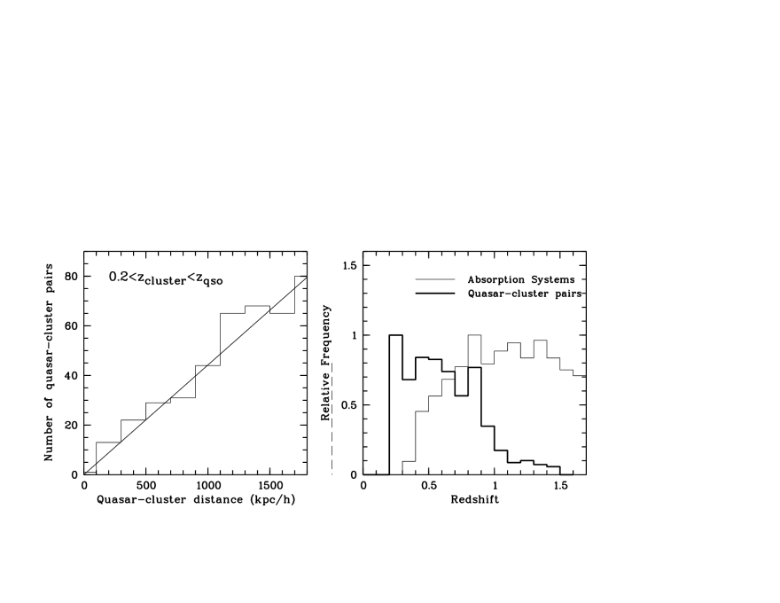
Figure 1: Left: Number of quasar-cluster pairs in the SDSS-RCS sample as a function of the projected physical distance between cluster and quasar line-of-sight at cluster redshift. The line is the expectation for constant projected number density of pairs. Right: Redshift distribution (normalized to maximum frequency) of clusters in the SDSS-RCS sample and of Mg II absorbers in Prochter, Prochaska & Burles (2006).

Fig. 1 shows the transverse-distance and cluster-redshift distributions of the SDSS-RCS sample. In the first one we plot the number of pairs found to have a given quasar-cluster distance. To see that this distribution results from a random distribution of clusters and quasars, we calculate the expected distribution (the stright line in the Figure) defining a mean density as the total number of pairs divided by the area of a circle of radius $2\,000$ $h^{-1}_{71}$ kpc. This comparison shows that all distances are well represented and that they roughly follow a uniform distribution, which is important for the homogeneity of the survey. The righthand panel of the Figure shows that the redshift distribution of Mg II systems found in SDSS quasar spectra (thin line; PPB06) and that of the SDSS-RCS sample have considerable overlap, meaning that our cross-correlation is well suited for searches of Mg II in cluster galaxies.

The SDSS-RCS sample of 442 quasar-cluster pairs is composed of 190 quasars and 368 clusters. Therefore, there are on average $\approx 2$ clusters per LOS, and $\approx 20$ % of the clusters are crossed by more than one LOS. Regarding observability, roughly $80$ % of the quasars are brighter than $g=20$ mag, and $\approx 50$ % of them are observable from Southern facilities.

2.2 New x-ray selected quasars

Since both galaxy clusters and quasars are ubiquitous x-ray emitters, using archival Chandra observations proved to be a successful way of selecting further targets for our study.

From the Chandra database we selected all public observations under the science category ‘Galaxy Clusters’. We imposed a maximum declination of $+20$ degrees, and a Chandra exposure time $\gtrsim 25$ ksec to ensure significant detections of the quasar candidates. The clusters also had to have a determined redshift above $z=0.2$. A final list of 29 observations that met these criteria were retrieved from the archive.

Next, we identified point-like sources in the x-ray data. We looked for candidate quasars located within a radius of $\lesssim 5\arcmin$ from the cluster central position. Since the observations were aimed at the cluster centers, we did not have to worry about the degradation of the Chandra point spread function with increasing off-axis distances. We then searched for optical point-like counterparts to the x-ray sources in SDSS images and obtained their $R$ and $B$ magnitudes from the APM catalog. Imposing the criteria $R>16$ and $B-R\lesssim 2.0$, a total of 49 candidate quasars were selected in 23 of the Chandra clusters. We will refer to this sample as the “x-ray sample”.

2.3 Pairs from the literature

A search in the NED was performed of quasars near RCS coordinates. Out of 7263 searches, 28 yielded quasars not found by the SDSS, that met the quasar-cluster criteria. We will refer to this sample as the “literature sample”. In addition, 5 other quasar-cluster pairs found in the literature were added to this sample. It is important to note that SDSS clusters are not well suited for our study due to their lower redshift ($z<0.3$; Koester et al. 2007).

3 Observations

3.1 Low-resolution spectroscopy

Low resolution optical spectroscopic follow-up observations of the quasar candidates from the x-ray sample were carried out with the Wide Field Reimaging CCD Camera in long-slit grism mode on the du Pont telescope at Las Campanas Observatory on March 30 and September 15-16, 2006. We used the blue grism, which gives a resolution of $\sim 3$Å and a wavelength range of $\sim 4700$Å.

Sixteen candidates were observed with enough signal-to-noise ratio to determine emission redshifts, and out of these, 7 quasars were confirmed. Other counterparts corresponded to Seyfert and star-forming galaxies, and a few stars (probably due to chance alignments). Therefore, the technique of using x-ray data to find quasars gave a success rate of $\approx 45$ %.

3.2 High-resolution spectroscopy

Echelle spectra were obtained using the MIKE spectrograph on the Las Campanas Clay 6.5m telescope. We obtained 18 quasar spectra in three runs on March 18-19 and September 23-24 and 29-30, 2006. Twelve of the quasars are from the SDSS-RCS, 2 from the x-ray, and 4 from the literature samples. The target selection was based only on airmass and brightness, i.e., without consideration of cluster redshifts. The observed sample represents $\approx 15$ % of the total number of available targets in the three samples.

Weather conditions were good but quite variable for two of the runs. Seeing ranged from good ($1\arcsec$) to excellent ($0.6\arcsec$). We made best efforts to obtain a S/N ratio as homogeneous as possible throughout the sample.

MIKE is mounted on the Nasmyth port and the slit orientation on the plane of the sky is fixed. For long exposures, and despite a low airmass, this requires manual corrections to keep the object centered on the slit, a task that proved feasible in general but difficult to carry out for some mag $\approx 20$ targets. For five of our targets we used integration times in excess of 4 hours. All spectra were taken with a $1\arcsec$ slit and an on-chip binning of $2\times 3$ pixels. With this setup the final spectral resolution of our spectra was $\approx 12.0$ and $\approx 13.5$ km s^-1 (FWHM) for the blue and red arms, respectively.

To extract the spectra we used our own pipeline running on MIDAS. The two-dimensional echelle spectra were flat-fielded (using star spectra taken with a diffusor) and extracted optimally (fitting the seeing profiles and taking into account the spatial tilts introduced by the cross-dispersing prisms). The orders were then calibrated with spectra of a Thorium-Argon lamp (using typically 15-20 lines per echelle order) and the different exposures co-added using a vacuum-heliocentric scale with $\Delta\lambda=0.067565$ and $0.1447107$ Å for the blue and red orders, respectively. Finally, the orders were normalized and merged. The spectral coverage of each spectrum is $\lambda=3\,350$ to $7\,480$ Å. Table 1 summarizes the echelle observations.

4 Sample Definitions and Redshift Path Density

In what follows we describe the various statistical samples drawn from the data. These samples were derived from the data on absorbers (see Table 2) and clusters (Table 3). We define the ’cluster redshift-path’ of the survey and the sample of ’hits’, or absorption systems found in the cluster redshift-path (summarized in Tables  4 and 5).

4.1 Sample of Mg II Absorption Systems

4.1.1 Mg II in High-resolution Spectra (Sample ’S1’)

The 18 MIKE spectra along with one UVES spectrum from the Literature Sample define what we shall call the ’high-resolution sample’, hereafter ’S1’. As in previous high-resolution surveys (e.g., Narayanan et al. 2007), we searched visually for Mg II systems in S1 by carefully scanning redshift chunks all along the range of Mg II detectability, each time plotting in velocity both doublet lines. We considered lines detected at the $3\sigma$ level or higher in both doublet lines.

Table 2 presents the absorption line data (LOS up to entry 19 in S1). Absorption redshifts are determined to within $\delta z_{\rm abs}\sim 10^{-4}$. rEW were calculated using pixel integrations with $1\sigma$ errors from propagated pixel variances. Lines within a velocity window of $500$ km s^-1 were considered one system, to conform to previous QAL surveys. Column ’$z_{\rm EW}$’ displays the minimum redshift at which a line with $W_{0}=0.05$ Å can be detected at the $3\sigma$ significance level. This value was computed assuming the error in the observed rEW is given by $\sigma_{W}={\rm FWHM}/\langle S/N\rangle$ (Caulet 1989), which holds when the spectral resolution dominates over the line width, as is our case. Since the spectra have increasing S/N with wavelength, there is no need to define a maximum redshift for the sake of the rEW threshold.

We found a total of $44$ systems with $0.015<W_{0}(2796)<2.028$ Å, $4$ of them with $W_{0}(2796)>1$ Å (LOS 5, 6, 15, and 18). Out of these 4, two are reported in the Mg II survey by PPB06 (see below), and two are new.

4.1.2 Mg II in Low-resolution Spectra (Sample ’S2’)

Out of the 190 quasars in the SDSS-RCS sample, 144 form 375 pairs where a Mg II system with $0.35<$$z_{\rm abs}$$<0.9$ can be found. We shall call these quasars the ’low-resolution sample’, hereafter ’S2’. Note that S1 and S2 are not disjoint, since several quasars in S2 were observed at high resolution.

To find Mg II absorbers in S2 we cross-correlated the sample with two extant SDSS Mg II samples: the sample by PPB06, comprising 7421 absorbers with $W_{0}(2796)>1.0$ Å, and the sample by BMPCW06, made of 1806 absorbers with $W_{0}>0.3$ Å. PPB06 surveys the redshift range $z_{\rm abs}$$\sim 0.35-2.3$ and BMPCW06 has $z_{\rm abs}$$\sim 0.37-0.8$. Both samples resulted from searches in DR3 spectra. In the cross-correlation we imposed the criteria $z_{\rm abs}$ $\leq 1.42$. This limit is given by the highest cluster redshift in the SDSS-RCS sample (but note that we will later restrict the statistical samples to much lower redshifts).

Out of the 144 quasars in S2, 22 are reported in PPB06 to show at least one strong ($W_{0}(2796)>1$ Å) Mg II system in the SDSS spectrum. Out of these, one is in a quasar that is paired with a cluster at too low a redshift and was therefore excluded. Out of the remaining 21 quasars in PPB06, two were observed at high resolution and therefore are also included in S1. The remaining 19 quasars show 21 systems that are listed in Table 2 along with absorption redshifts and rEW from PPB06 (LOS 20 and beyond). Let us emphasize that the two systems in LOS 15 and 18 of S1 are reported also by PPB06, so there is a total of 23 Mg II systems with $W_{0}>1$ Å in S2 (in the LOS 15, 18, 20 and beyond) that were reported by PPB06. The two other $W_{0}>1$ Å systems in S1 (LOS 5 and 6) are not reported in PPB06.

Out of the 144 quasars in S2, 5 are reported in BMPCW06 to show at least one Mg II system with $W_{0}>0.3$ Å in the SDSS spectrum. Out of these, 4 with $W_{0}>1$ Å are in the PPB06 sample (though 2 of these, 092746.94+375612 and 141635.78+525649, with rEW differing by $\approx 30$ %) and only one has $0.8<W_{0}<1.0$ Å. We decided not to include this latter system into our statistics because the redshift range surveyed by BMPCW06 is shorter than we can probe with our quasar-redshift pairs. Therefore, only the PBB06 results were used in our statistics. However, after calculating rEW values for the two systems with disagreeging rEW in the two surveys, we decided —for these two particular systemsç— to use the values reported by BMPCW06, which better match ours (this choice has consequences for the rEW distribution below).

4.2 Sample of Clusters and Survey Redshift Path

4.2.1 Cluster Redshift Intervals

Table 3 displays the cluster data for each LOS that contains absorption systems (same numbering as in Table 2). The 19 quasar spectra in S1 define a sample of 46 clusters with redshifts between $z_{\rm cluster}$$=0.173$ and $1.085$. Out of these, 37 are drawn from the SDSS-RCS sample, 2 from the x-ray sample and 7 from the literature sample. In S2 all clusters come from the RCS.

RCS cluster redshifts are photometric and estimated to within $\delta z=0.1$ in this redshift range (Gilbank et al. 2007). The other 9 clusters have spectroscopic redshifts and we will assume $\delta z=0.01$, which corresponds to $\Delta v=2\,000$ km s^-1 at $z_{\rm cluster}$$\sim 0.5$. Since we will analyze absorption systems with $z_{\rm abs}$$\sim$$z_{\rm cluster}$, our survey’s redshift path will be defined by what we shall call ’redshift intervals’ around each quasar-cluster pair. These are in turn defined as $[z_{\rm min},z_{\rm max}]$, with $z_{\rm min}=$$z_{\rm cluster}$$-\delta z$ and $z_{\rm max}=$$z_{\rm cluster}$$+\delta z$, unless $z_{\rm min}<z_{\rm EW}$, in which case we set $z_{\rm min}=z_{\rm EW}$. This choice implies that every redshift interval in S1 permits a $>3\sigma$ detection of a system with $W_{0}>0.05$ Å (this choice has also consequences on survey completeness as explained below in § 6.2). No cluster has $z_{\rm max}<z_{\rm EW}$, so no redshift interval was excluded from S1. Recall that, in general, the number of redshift intervals is not equal to the number of clusters, since some clusters are crossed by more than one LOS.

For redshift intervals associated with S2 we set $z_{\rm EW}=0.35$, which defines a rEW threshold of $W_{0}^{\rm min}=1.0$ Å. With this cut, out of the 442 quasar-cluster pairs in the SDSS-RCS sample, 375 remain in S2. These pairs are associated with 144 LOS. In Table 3 (LOS 20 and beyond) we show only clusters associated with the 19 quasars in S2, besides LOS 15 and 18, that show a Mg II system with $W_{0}>1$ Å.

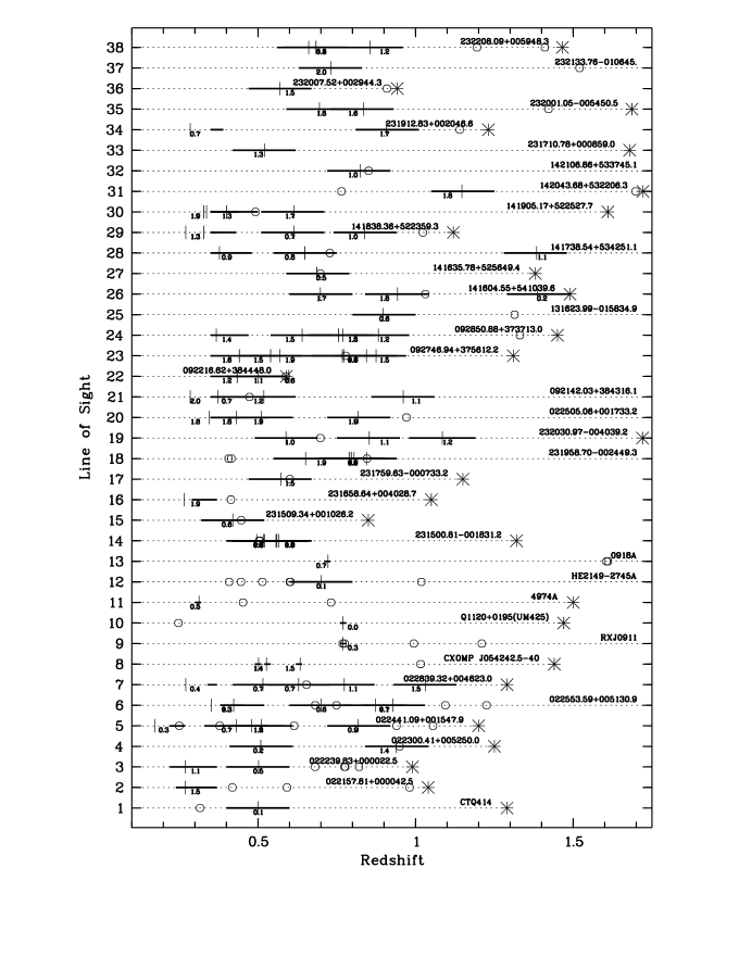
Figure 2: Diagram of the subset of lines of sight (LOS) toward which Mg II absorption systems were found. The LOS numbering is the same one used in Tables 2 and 3. LOS up to 19 belong to sample S1; LOS 20 to 38 to sample S2. Quasar emission redshifts are labeled with asterisks, Mg II absorption systems with circles, and clusters with vertical lines. The thick lines despict the redshift intervals [$z_{\rm min},z_{\rm max}$] around cluster redshifts. These intervals permit a $3\sigma$ detection of Mg II $\lambda 2796$ lines with $W_{0}>W_{0}^{\min}=0.05$ Å in S1 and with $W_{0}>W_{0}^{\min}=1.0$ Å in S2. The numbers below the thick lines are the projected LOS-cluster distance in $h^{-1}_{71}$ Mpc at cluster redshift.

Fig. 2 shows a diagram of redshift intervals in each of the LOS. The LOS numbering is the same used in Tables 2 and 3. Quasar emission redshifts are labeled with asterisks, Mg II absorption systems with circles, and clusters with vertical lines. The thick lines depict the cluster redshift intervals. The numbers below the thick lines are the LOS-cluster distance (at $z_{\rm cluster}$) in $h^{-1}_{71}$ Mpc. LOS up to 19 belong to sample S1; LOS 20 to 38 to sample S2.

4.2.2 A New Definition of Redshift Path Density

In order to calculate the incidence of Mg II absorbers at cluster redshifts, $z_{\rm cluster}$, a function must be defined that accounts for the probability of detecting the doublet at a given redshift. In QAL surveys such a function is the Redshift Path Density $g(W_{\rm min},z_{i})$, which gives the number of sightlines (quasar spectra) in which an absorption system with rEW $W_{0}>W_{0}^{\rm min}$ might have been detected at redshift $z=z_{i}$ (see, for instance, Eq. [1] in Ellison et al. 2004a). Thus, in QAL surveys, $g(W_{\rm min},z_{i})$ provides the redshift path sensitivity of the survey and the total redshift path surveyed is given by:

$$\Delta z=\int_{0}^{\infty}g(W_{\rm min},z_{i})dz.$$ (1)

Since in the present analysis we are interested in the incidence of absorbers at cluster redshifts, the following conceptual modification has to be introduced: the redshift intervals defined in § 4.2.1, $[z_{\rm min},z_{\rm max}]$, will be treated as if they were ‘quasar spectra’, regardless of how many of them are present in one LOS. The reason for this choice is that having more than one cluster in the same LOS and at similar redshifts (overlapping clusters) increases the a priori probability of detecting an absorber in that particular LOS. Similarly, two different LOS through the same cluster add twice to the overall redshift path.

We therefore define a ‘cluster redshift path density’, $g_{c}(W_{0}^{\rm min},z_{i},d)$, as the function that gives the number of cluster redshift intervals within a LOS-cluster distance $d$, in which a $W_{0}>W_{0}^{\rm min}$ Mg II system at redshift $z_{i}$ might have been detected. The cluster redshift-path $\Delta$$z_{\rm cluster}$ between any two redshifts $z_{1}$ and $z_{2}$ is thus

$$\Delta z_{\rm cluster}(W_{0}^{\rm min},z_{1},z_{2},d)=\int_{z_{1}}^{z_{2}}g_{c}(W_{0}^{\rm min},z,d)dz.$$ (2)

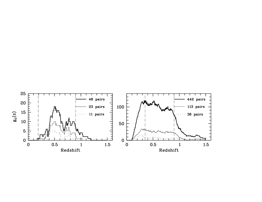
Figure 4: Cluster redshift-path density, $g_{c}(W_{0}^{\rm min},z_{i})$ of the high-resolution sample (S1, $W_{0}^{\rm min}=0.05$ Å, lefthand panel) and low-resolution sample (S2, $W_{0}^{\rm min}=1.0$ Å). The thick line is for LOS-cluster distances $d<2$, the thin line for $d<1$, and the dotted line for $d<0.5$ $h^{-1}_{71}$ Mpc. The vertical dashed lines depict the redshift defined by the rEW detection thresholds. See § 4.2.2 for more details.

In Fig. 4 we show $g_{c}(z)$ for the two samples. Note that $g_{c}(z)$ is not only different for each of the samples (because of different rEW thresholds) but also for each cut in distance. Sample S1 provides a cluster redshift path between $z=0.2$ and $z=0.9$ of $\Delta$$z_{\rm cluster}$$=6.3$ for $d<2$ $h^{-1}_{71}$ Mpc. This is the longest path available for searches of lines as weak as $W_{0}=0.05$ Å. In the redshift interval [0.35,0.90] and for $W_{0}>1$ Å, sample S2 provides a redshift path of $\Delta$$z_{\rm cluster}$$=57.0$ for $d<2$ $h^{-1}_{71}$ Mpc. Overlaps represent $\approx 40$ % of the total redshift path for clusters at $d<2$ but only $\approx 10$% for $d<1$ $h^{-1}_{71}$ Mpc. These numbers are summarized in Table 4.

4.3 Sample of Mg II absorbers at cluster redshifts: ’hits’

We shall call an absorber a ‘hit’ when $z_{\rm abs}$ is in a cluster redshift interval. The function $N_{\rm hit}$=$N_{\rm hit}$$(z_{1},z_{2},W_{0},d)$ is defined as the number of hits between redshifts $z_{1}$ and $z_{2}$ with a given cut in rEW and distance. $N_{\rm hit}$ enters in the definition of $dN/dz$ below. We recall that (1) there may be more than one hit in one redshift interval (two absorbers in the same LOS through the same cluster); (2) there may be more than one hit in one cluster (two absorbers in different LOS through the same cluster); and (3) redshift intervals may overlap (thus increasing the probability of getting a hit). Table 5 summarizes the hits for the two samples and various cuts in rEW and $d$.

The following caveat must be considered: overlapping redshift intervals have no one-to-one correspondence with hits; in other words, we lack information as of which one of the overlapping clusters is responsible for the absorption. This degeneracy, however, has a minor effect on the results by cluster impact parameter, since there are only two cases in the whole sample (LOS 5 and LOS 14) where a hit occurs in two overlapping intervals, with one being at $d<1$ and the other one being at $1<d<2$ $h^{-1}_{71}$ Mpc. These particular hits were assigned to both statistics: $d<1$, and $d<2$ $h^{-1}_{71}$ Mpc.

4.4 Redshift Number Density of Absorbers in Galaxy Clusters

To study the incidence of Mg II in cluster galaxies we define — similarly to an unbiased QAL survey defined by $W_{0}^{\rm min}$ — the redshift number density of absorbers in galaxy clusters, $(dN/dz)_{c}$, as the number of hits per unit cluster redshift:

$$(dN/dz)_{c}(W_{0},z_{1},z_{2})\equiv\frac{N_{\rm hits}(W_{0},z_{1},z_{2})}{\Delta z_{c}(W_{0},z_{1},z_{2})},$$ (3)

and its rEW distribution, $n_{c}(W_{0})\equiv\frac{d^{2}N}{dWdz}$, as the number of hits per unit cluster redshift per unit EW, such that:

$$\int_{W1}^{W2}n_{c}(W_{0},z_{1},z_{2})dW=(dN/dz)_{c}.$$ (4)

The errors are calculated assuming Poisson statistics, for which we use the tables in Gehrels (1986).

These two observational quantities, $(dN/dz)_{c}$ and $n_{c}(W_{0})$ must be proportional to the average number density of absorbers in a cluster, $n_{c}(z)$, and their cross-section, $\sigma_{c}(z)$:

$$(dN/dz)_{c}\propto n_{c}(z)~{}\sigma_{c}(z)~{}.$$ (5)

Although in general $(dN/dz)$ has been used to study how absorbers evolve, our samples are rather small and we just focus on a possible overdensity $\delta$ of absorbers with respect to the field. We define

$$\delta\equiv(dN/dz)_{c}/(dN/dz)_{f}~{},$$ (6)

where $(dN/dz)_{f}$ is the incidence of systems in the field. We compare the two distributions measured in clusters with the following field Mg II surveys: NTR06 (MMT telescope spectroscopy, spectral resolution FWHM $\approx 2.2$ Å; rEW threshold $W_{0}^{min}=0.1$ Å), NTR05 (SDSS EDR, FWHM $\approx 4$ Å, $W_{0}^{min}=0.3$ Å), CRCV99 (Keck HIRES, FWHM $\approx 0.15$ Å, $W_{0}^{min}=0.02$ Å), and Narayanan et al. (2007; VLT UVES, FWHM $\approx 0.15$ Å, $W_{0}^{min}=0.02$ Å). Other surveys have redshift intervals that do not match ours (Lynch, Charlton & Kim 2006).

These surveys have found (1) that weak and strong systems show different rEW redshift distributions: weaker systems are fitted by a power-law while stronger systems are better described by an exponential, with the transition at $W_{0}\approx 0.3$ Å. This effect would hint at two distinct populations of absorbers (e.g., NTR05); (2) little evolution of any of the populations between $z\approx 1.4$ and $0.4$ (Narayanan et al. 2007; Lynch, Charlton & Kim 2006). The nature of weak ($W_{0}<0.3$ Å) Mg II is not clear yet. It has been suggested that single-cloud systems may have an origin in dwarf galaxies due to their abundances (Rigby et al. 2002) or to their statistics (Lynch, Charlton & Kim 2006); they might also be the high-redshift analogs to local HVCs (Narayanan et al. 2007, and references therein). Unfortunately, there exist only few QAL surveys of weak Mg II systems, mainly due to the more scarce high-resolution data.

5 Results: The Incidence of Mg II in Galaxy Clusters

In this section we present the results on $(dN/dz)_{c}$ and $n_{c}(W_{0})$ as observed in S1 (for systems having $W_{0}<1.0$ Å) and S2 ($W_{0}>1.0$ Å). For both samples we analyze pairs with $d<2$ and $<1$ $h^{-1}_{71}$ Mpc separately, and we restrict the statistics to $z<0.9$, where the cluster sample is more reliable. Finally, we re-analize S2 taking into account two refinements of the method, namely selection by cluster richness and the redshift-dependence of $\delta z$.

5.1 $W_{0}<0.3$ Å  systems

The parameterization by CRCV99 of their Keck HIRES data implies $(dN/dz)_{f}=1.41$ at $\langle z\rangle=0.65$ for field systems with $0.02<W_{0}<0.3$ Å at $0.4<z<1.4$. This is consistent with the results by Narayanan et al. (2007) at that redshift and in the same rEW interval using UVES data.

For our redshift intervals having $d<1$ $h^{-1}_{71}$ Mpc we find $(dN/dz)_{c}=1.20$ ([0.37 2.70] $1\sigma$ c.l.) for $0.05<W_{0}<0.3$ Å and binning in the range $0.2<z<0.9$. Given that our data are complete only down to $W_{0}=0.05$ Å, we cannot compare directly with the value by CRCV99. Therefore, we apply a downward correction to this value of $23.3$ %, which is the fraction of systems with $0.02<W_{0}<0.05$ Å in the CRCV99 sample. After this correction, the field value is $(dN/dz)_{f}=1.09$, which is in good agreement with $(dN/dz)_{c}$. For the $d<2$ $h^{-1}_{71}$ Mpc sample we find a somewhat smaller value of $(dN/dz)_{c}=0.79$ ([0.29 1.64] $1\sigma$ c.l.) that is however still consistent with the field measurement.

5.2 $W_{0}>0.3$ Å  systems

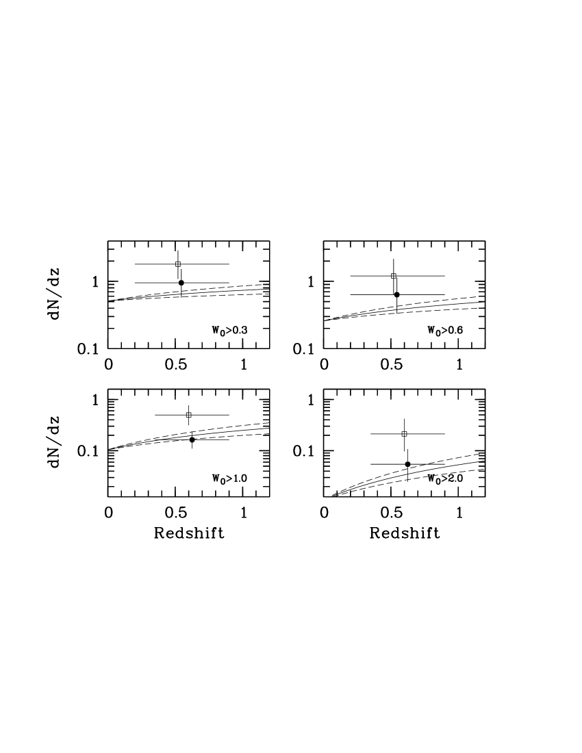
Figure 5: Mg II redshift number density binned in the entire range of cluster redshifts for various $W_{0}^{2796}$ lower limits. The filled circles are from clusters with LOS-cluster distances $d<2$ $h^{-1}_{71}$ Mpc and the open squares from clusters with $d<1$ $h^{-1}_{71}$ Mpc (symbols slightly shifted in the x-axis for more clarity). The errors bars correspond to $1\sigma$. The curves correspond to the fit by NTR05 to their SDSS EDR data of field absorbers along with $1\sigma$ limits. The top panels show results from sample S1 only (high-resolution spectra; 46 pairs, $\langle z\rangle$$=0.550$), while points in the bottom panels were calculated using only the S2 sample (375 pairs; $\langle z\rangle$$=0.625$).

Figure 5 shows the cumulative values of $(dN/dz)_{c}$ (and their $1\sigma$ errors) for systems with $W_{0}>0.3$ Å. We bin in the ranges $0.2<z<0.9$ (top panels) and $0.35<z<0.9$ (bottom panels). The top panels show results from sample S1 only (46 quasar-cluster pairs, $\langle z\rangle$$=0.550$), while points in the bottom panels were calculated using sample S2 (375 pairs; $\langle z\rangle$$=0.625$). The filled circles are for clusters at distances $d<2$ $h^{-1}_{71}$ Mpc from quasar LOS and the open squares represent clusters with $d<1$ $h^{-1}_{71}$ Mpc (symbols are slightly shifted in the x-axis for more clarity). The curves correspond to the fit by NTR05 to their EDR data of field absorbers with $1\sigma$ limits calculated as described in the Appendix of their paper. These fits are in excellent agreement with the SDSS data of field Mg II absorbers.

There is an overdensity of hits per unit redshift in clusters compared with the field population for $d<1$ $h^{-1}_{71}$ Mpc clusters; the $d<2$ $h^{-1}_{71}$ Mpc sub-samples instead, are consistent with the field statistics. In addition, the data show that $\delta$ is larger for stronger systems ($W_{0}>2.0$ Å) than for weaker systems. These two trends are more clearly seen in Table 5, where we compare the measured value of $(dN/dz)_{c}$ with the field, for various rEW ranges (using cosmic averages from different authors). Note that the confidence limits listed in the Table for $(dN/dz)_{c}$ are $2\sigma$ only. The overdensity effect for $d<1$ $h^{-1}_{71}$ Mpc ($W_{0}>1$ and $W>2$ Å cuts) is significant at the 99% level or slightly higher. For $d<0.5$ $h^{-1}_{71}$ Mpc we also note the overdensity of stronger systems, though the effect here is only $1\sigma$ due to the small number of hits.

5.3 Mg II $\lambda 2796$ equivalent width distribution

5.3.1 Stronger (Weaker) Systems in Clusters are (not) Overdense

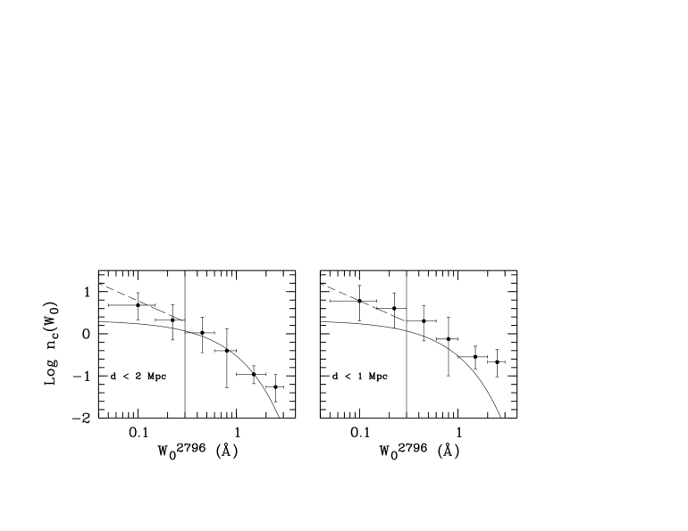
Figure 6: Equivalent width distribution of Mg II absorbers in clusters (corrected by the cluster redshift path) vs. Mg II $\lambda 2796$ rest-frame equivalent width for LOS-cluster distances $d<2$ $h^{-1}_{71}$ Mpc (lefthand panel) and $d<1$ $h^{-1}_{71}$ Mpc. The errors bars correspond to $1\sigma$. Data points with $W_{0}<1.0$ Å resulted from sample S1 only (high-resolution spectra), while points at $W_{0}>1.0$ Å resulted from sample S2. The lines are the field expectations. The solid line is the exponential distribution fitted by NTR06 to their MMT data having $W_{0}>0.3$ Å, and the dashed curve is the power-law fited by CRCV99 to their HIRES data having $W_{0}<0.3$ Å. The vertical line at $W_{0}=0.3$ Å marks the transition in $n(W)$ pointed out by NTR06.

Fig. 6 summarizes our main result. It shows $n_{c}(W_{0})$ and $1\sigma$ errors for Mg II systems at $d<1$ and $d<2$ $h^{-1}_{71}$ Mpc from a cluster. Data points with $W_{0}<1.0$ Å result from sample S1 only, while points at $W>1$ Å are calculated using S2 only. The solid curve is the exponential distribution $n(W_{0})=N^{*}/W^{*}\exp{-W_{0}/W^{*}}$ fitted by NTR06 to their MMT data for $W_{0}>0.3$ Å (114 Mg II systems, $\langle z\rangle$$=0.589$). The parameters are $W^{*}=0.511$ and $N^{*}=1.071$ and the fit is in excellent agreement with their data having $0.5\lesssim W_{0}\lesssim 3.0$ Å (see their Fig. 2). The dashed curve is the power-law fit, $n(W_{0})=0.55~{}W_{0}^{-1.04}$ fitted by CRCV99 to their Keck HIRES data. The power-law is in excellent agreement with their $W_{0}\lesssim 0.3$ Å data and also with data by Steidel & Sargent (1992), but clearly overestimates the MMT and SDSS/ERD data for larger $W_{0}$.

Fig. 6 confirms the excess of strong ($W_{0}\gtrsim 1.0$ Å) Mg II systems near cluster redshifts, when compared with the field population. On the contrary, the weaker systems ($W_{0}\lesssim 0.3$ Å) conform to the field statistics. Furthermore, this effect seems more conspicuous for the $d<1$ $h^{-1}_{71}$ Mpc sample than for the $d<2$ $h^{-1}_{71}$ Mpc sample, which shows a slight overdensity only for stronger systems. The weak systems are also consistent with other QAL surveys. For instance, the results by Narayan et al. (2006) for the $0.4<z<1.4$ range are in good agreement with ours (their Fig. 7) even for our $d<1$ $h^{-1}_{71}$ Mpc sample, considering a $29.3$ % downward correction to their $n(W_{0})$ values due to our smaller rEW range of [0.05,0.3] Å. On the contrary, for $d<1$ $h^{-1}_{71}$ Mpc, $n_{c}(W_{0})$ is overabundant by a factor of $\approx 3$ in the [1.0,2.0] bin and $\approx 15$ in the [2.0,3.0] bin (note Table 5 shows a comparison with NTR05). The latter result is significant at the $>3\sigma$ level (assuming no errors in the field average).

Summarizing, stronger systems ($W_{0}\gtrsim 1.0$ Å) are overdense in clusters; weaker systems ($W_{0}\lesssim 0.3$ Å) are not. This makes $n_{c}(W_{0})$ appear flatter than $n(W_{0})$ (on a log-log plot) and much better fitted by a power-law, also in the large-rEW end, than by an exponential.

5.3.2 Is the Effect Real?

The different behaviour of strong and weak systems cannot be due to the different redshift paths $\Delta z_{c}$ of S1 and S2. If this were the case, the offset in $(dN/dz)_{c}$ should be equal in the entire rEW range; however, we see that the statistics is affected differentially.

Another possible caveat is that an incomplete survey in the small-rEW end would as well have an effect on the differential behaviour of $n(W_{0})$ between weak and strong systems (weaker lines are more difficult to find). However, the [0.05,0.3] bin has 4 absorbers in S1, meaning that to get a factor of say $10$ more systems per unit rEW in that bin we should have missed 36 hits, which is quite unlikely ($10^{-12}$ for a Poisson distribution).

The stronger effect seen for $d<1$ when compared with $d<2$ $h^{-1}_{71}$ Mpc is clearly influenced by the shorter redshift path in the former selection. Indeed, from Table 5 we see that the transition from $d<2$ to $d<1$ $h^{-1}_{71}$ Mpc, is more or less governed by the change in $\Delta$$z_{\rm cluster}$ (i.e., the number of hits do not change much). We take this as a possible evidence that the data is sensitive to a typical cluster only at distances below $1$ $h^{-1}_{71}$ Mpc. Further support for this idea is that the $d<0.5$ $h^{-1}_{71}$ Mpc overdensities, though at low significance, do not scale with $\Delta$$z_{\rm cluster}$.

Finally, let us note that our definition of $\delta$ and the large radial distances implied by the photometric redshift accuracy ($\delta z$) imply that $\Delta z_{\rm cluster}$ may (and probably does) include some level of contamination by field absorbers. Consequently, what the present cluster data allows us to state is that regions that contain a cluster do show more strong absorbers than the cosmic average, while for weak systems those regions are indistinguishable from the field.

5.4 Refinements

5.4.1 Selecting by Cluster Richness

In the current analysis we have included all the objects in our RCS catalog, constraining its significance to be greater than $3\sigma$ (Gladders and Yee 2000). This threshold is low enough to detect almost all the clusters in the RCS areas, but presumably it also includes low mass groups and even some spurious detections. On the other hand, this selection has the great feature that allows us to cross correlate a large number of objects, but also it has the drawback that any signal we detect in the absorption systems might be diluted by low mass objects or spurious clusters.

In order to quantify the extent of this ’dilution’ we have selected a subsample of clusters with a more stringent criteria given by a minimum richness (that translates into a minimum mass). So far we have used sample S2 that has a median $B_{gc}$ of 263 that translates into a mass of $\approx 2.4\times 10^{13}M_{\odot}$ (Blindert et al., in prep.). Similar values are obtained for the subsample having $d<1$ $h^{-1}_{71}$ Mpc.

The more restricted sample, which we call ’S2-best’ is required to have only clusters with $B_{gc}\geq 350$. This selection includes only 125 quasar-cluster pairs for an impact parameter of at least 2 $h^{-1}_{71}$ Mpc, and a median $B_{gc}$ of 488 that translates into a mass of $8.8\times 10^{13}~{}M_{\odot}$. Similarly, we find a median $B_{gc}$ of 478 for a $d<1$ $h^{-1}_{71}$ Mpc. As shown in Table 5, repeating the analysis of hits using S2-best yields higher overdensities —by $\sim 50$%— than for S2 for the same rEW ranges. Most importantly, despite a much lower redshift path, the significance of the result is still high ($>3\sigma$).

Sample S1 has fewer quasar-cluster pairs and only a few of the clusters come from the RCS sample. For these objects we find a median $B_{gc}$ of 327 for an impact parameter of 2 Mpc and 258 for the smaller aperture, i.e., consistent with the larger sample. Therefore, a similar analysis for S1 was considered not worth performing due to the few clusters in that sample. However, we note that the median $B_{gc}$ is not particularly low, so this sample is also representative of more massive clusters (i.e., the lack of overdensity is not due to a chance conjunction of low mass systems).

Concluding, finding a significantly stronger signal in clusters selected by a mass proxy gives strong support to both the method and the reliability of the systems used in the analysis. In fact, the richness selection not only provides more galaxies per clusters but also picks up larger clusters. Both selection effects are expected to increase the a priori hit probability.

5.4.2 Cluster Redshift Accuracy

Since our comparison between cluster and field Mg II statistics depends on the definition of redshift intervals, we have to consider what effect the cluster redshift accuracy may have on our results. For clusters with spectroscopic redshifts we have assumed $\delta z=0.01$. If due to the Hubble flow, this translates into a radial distance of $67$ comoving Mpc; therefore, one might want to shorten $\delta z$ to overcome the problem of contamination by field absorbers. Unfortunately, the redshift path provided by the pairs with spectroscopic cluster redshifts represents only $\approx 2$ % of $\Delta z_{\rm cluster}$. Since shortening to $\delta z=0.005$ does not exclude the only hit (LOS 9) at a spectroscopic $z_{\rm cluster}$, $(dN/dz)_{c}$ remains practically unchanged.

The vast majority of our clusters have photometric redshifts and our analysis assumes $\delta z=0.1$ for those ones. This is indeed an over-estimate for the lower-redshift clusters, $z_{\rm cluster}$$\lesssim 0.5$, where the accuracy can be as good as $\delta z\approx 0.04$. In order to see whether a smaller $\delta z$ would affect the results on $(dN/dz)_{c}$ we use the parameterization $\delta z=0.04(1+z_{\rm cluster})$ and re-compute $g_{c}(z)$ and $N_{\rm hits}$. Restricting the analysis to $d<1$ $h^{-1}_{71}$ Mpc pairs in S2 (where the overdensity signal is most evident), we find that out of $7$ hits with $W_{0}>1$ Å only one hit (LOS 28, $W_{0}=1.58$ Å) is ruled out due to the shorter redshift intervals. Since the new $\delta z$ makes the total redshift path between $z=0.35$ and $z=0.9$ decrease to $\Delta z_{\rm cluster}=9.18$, we find actually a higher overdensity of $\delta\approx 4$ and $\delta\approx 10$ for $W_{0}>1.0$ and $1.0<W_{0}<2.0$ Å, respectively. We conclude that our result is indeed affected by a more precise parameterization of the RCS redshifts but such refinement makes the signal even stronger. In order to avoid fine-tuning too many variables, we continue the analysis of the results using a constant $\delta z$.

6 Statistical Significance, Possible Biases, and Caveats

Despite the strong test provided by the mass selection, our method might still suffer from possible systematics and biases hidden in the statistical properties of the various samples. We analyze these in what follows.

6.1 Statistical Significance

We start by asking whether the detected overdensity might be due to chance alignments. To assess the statistical significance of the observed number of hits one might want to run Monte Carlo simulations by creating samples of random cluster redshifts. However, this is equivalent to calculating $dN/dz$ from random sub-samples drawn from the parent quasar sample (i.e., creating random RCS-SDSS samples). Such kind of simulations must, by definition, yield the cosmic value obtained by QAL surveys, a number against which we have compared our resuls. To see whether we recover the expected number of field absorbers, we calculate $(dN/dz)_{f}$ in the complementary redshift path of our quasar-cluster sample, that is, the path that does not include clusters. If our sample is biased toward an overdensity of absorbers for reasons other than the presence of clusters we should get an overdensity here too; if it is not, we should recover the field value. We analyze quasars in sample S2, the one that yields the overdensity, and split it into two redshift ranges: $z=$[0.35,0.9], the one used to get $(dN/dz)_{c}$, and $z=$[0.9,1.4]. The latter was not used in the analysis of cluster absorbers but may be a useful check for unbiased LOS.

There are $85$ quasars in S2 that provide cluster redshift intervals at $d<1$ $h^{-1}_{71}$ Mpc, where $W_{0}>1$ Å Mg II systems may be detected. Between $z=0.35$ and $0.9$ the total quasar redshift path of this sample is $\Delta z_{\rm quasar}=45.15$, so the complementary redshift path is $\Delta z_{\rm field}=\Delta z_{\rm quasar}-\Delta z_{\rm cluster}=45.15-14.13=31.02$, where we have subtracted the cluster path $\Delta$$z_{\rm cluster}$$=14.13$ (see Table 5).

The expected number of $W_{0}>1.0$ Å systems along $\Delta z_{\rm field}$ is thus $5_{-2.2}^{+3.4}$ and the expected number of systems with $2.0<W_{0}<3.0$ Å is $0_{-0}^{+1.9}$ ($1\sigma$ errors). From Tables 2 and 5, the observed number of systems along $\Delta z_{\rm field}$ in this redshift range is: [# systems in RCS-SDSS] $-$ $N_{\rm hits}$ = $10-7=3$ for $W_{0}>1.0$ Å and $3-3=0$ for $2.0<W_{0}<3.0$ Å systems (i.e., no system with $2.0<W_{0}<3.0$ Å was expected in the field and no system was observed in the field, with the 3 other systems all being hits). These values are in agreement with the field expectation.

Repeating the above analysis for the $z=$[0.9,1.4] range, we get: $\Delta z_{\rm quasar}=31.38$, $\Delta$$z_{\rm cluster}$$=3.00$, number of expected field absorbers: $7_{-2.6}^{+3.8}$, number of detected field absorbers: 8 (total) - 1 (hit) = 7, i.e., again within the field expectation. We conclude that the observed overabundance of strong Mg II systems is not due to chance alignments and must reflect real overdensities. In other words, sample S2 of quasars is biased only by the presence of clusters. The bias vanishes at redshifts other than $z_{\rm cluster}$, where we recover the cosmic statistics obtained in QAL surveys (the presence of clusters in these surveys has negligible influence on such statistics).

6.2 Yet More Possible Biases and Caveats

6.2.1 Clusters and Quasars

Besides the obvious fact that the completeness of our cluster sample — drawn mainly from the RCS — depends on the RCS algorithm, it is important to stress that the parent cluster and quasar samples are totally independent each from the other. The RCS sample is certainly not complete for S2 (particularly at higher redshifts), which includes low mass systems, but it is for S2-best up to $z\lesssim 1$, which includes moderately massive clusters. On the other hand, the SDSS quasar sample should be $\sim 90$ % complete (York et al. 2000). These and the arguments given in § 2.1 lead us to conclude that the SDSS-RCS sample, and thus also sample S2-best of pairs, is complete and homogeneous, at least at the same level as their parent surveys.

Another obvious strength of the quasar-cluster sample is that the search of absorbers in S2 (PBB06; BMPCW06) was performed independently of our selection. This is not completely true for S1 since those quasars were selected for follow-up spectroscopy after the quasar-cluster selection. However, at the telescope, the targets were selected without prior knowledge of cluster redshifts; moreover, even if this had been the case, the low-resolution spectra provided by the SDSS do not permit an a priori selection of weak systems. Therefore, there was no way to prefer quasars with absorbers. We discuss this further below in the context of absorber statistics.

Finally, the following caveat must be mentioned: brighter quasars are chosen for spectroscopy, which might be amplified by gravitational lensing by the absorber host galaxies (see discussion in § 8).

6.2.2 Absorbers

Surveys of quasar absorption-line systems assess the completeness of the samples via cumulative $\Delta z$ as a function of rEW threshold (Steidel et al. 1992). Since we have chosen our redshift path to include only spectral regions sensitive to $W_{0}>0.05$ Å, we consider the sample S1 of absorbers to be nearly 100% complete. Similarly, we assume that S2 is statistical in the sense that all Mg II systems with $W_{0}>1.0$ Å were listed in PPB06, who argue that their search is $>95$ % complete.

As for the homogeneity of the samples, we have kept S1 and S2 carefully separated. Again, out of the 4 $W_{0}>1$ Å systems found in S1, we have considered in S2 only those two found by PBB06 (including the remaining two would increase $\delta$ since one system is a hit).

Admittedly, one concern is that detecting an overdensity in one sample and not in the other may reflect a hidden systematic. We do not have at this time the means of testing such possible systematics. If we use only S1 in the $W_{0}>1$ Å range we also find an overdensity with respect to the field, although with low significance: $1$ hit is expected while $2$ are found. However, as pointed out above, these statistics may be influenced by the fact that quasars in S1 were selected as having a cluster in the LOS, and strong systems are readily seen in the SDSS spectra. However, weak systems are not seen in the SDSS and we know they do not cluster around stronger systems (CRCV99). In addition, if there were in fact such hidden systematics, why is not the supposedly biased sample (S1) the one that shows the overdensity? In other words, despite an obvious selection effect toward targets with clusters, S1 does yield the field statistics for weak absorbers.

Finally, note that the significance of our result for strong absorbers could increase if a larger cluster redshift path were surveyed. Tables 4 and  5 show that only roughly $3-4$% of the quasar-cluster pairs results in hits. This explains why an earlier attempt failed to detect strong Å Mg II systems in a sample of 6 Abell clusters (Miller, Bregman & Knezek 2002).

7 Summary of the Results

We have cross-correlated candidate galaxy clusters from the RCS at $z_{\rm cluster}$$=0.3$–$0.9$ with background quasars from the SDSS DR3 to investigate the incidence $(dN/dz)_{c}$ and rEW distribution $n_{c}(W_{0})$ of Mg II absorption systems associated with cluster galaxies. We have found 442 quasar-cluster pairs at impact parameters $d<2$ $h^{-1}_{71}$ Mpc from cluster coordinates, where Mg II might be detected in redshift regions $\pm 0.1$ from a cluster. The cluster sample contains all systems in the RCS, and is dominated by low-mass clusters and groups with $\langle M\rangle\sim 2\cdot 10^{13}$ M_☉ cluster candidates. We have defined a cluster redshift-path density in terms of the quasar-cluster pairs. Using extant surveys of strong Mg II systems in DR3 quasar spectra and our own follow-up high-resolution spectroscopy, we calculated $(dN/dz)_{c}$ and $n_{c}(W_{0})$ for the rEW range $0.05<W_{0}<3.00$ Å. The results were:

1. There is an excess of strong ($W_{0}^{2796}>1.0$ Å) Mg II absorbers near —i.e., at similar redshift of and close in projection to— galaxy clusters when compared to surveys in the field. The effect is significant at the $2\sigma$ level. This overdensity, $\delta\equiv(dN/dz)_{c}/(dN/dz)_{f}$, is also more pronounced at smaller distances ($d<1$ $h^{-1}_{71}$ Mpc) than at larger distances ($d<2$ $h^{-1}_{71}$ Mpc) from the cluster, which we interprete as a dilution of the effect in the field. On the other hand, the excess is also more pronounced for stronger systems. For $d<1$ $h^{-1}_{71}$ Mpc and $W_{0}=$ [2.0,3.0] Å, we measure $\delta\approx 6$–$15$ (depending on the field survey used for comparison), and the significance increases to $3\sigma$.

2. If we select the sample third with most massive (and significant) cluster candidates, we find the excess of absorbers increases by 50% for the sub-sample dominated by $\langle M\rangle\sim 10^{14}$ M_☉ clusters. The effect becomes also more significant, rendering reliability to our detection.

3. The weak population of Mg II systems ($W_{0}<0.3$ Å) in clusters conform to the field statistics. The absence of an overdensity is not due to lack of sensitivity. This effect and the excess of strong systems make $n_{c}(W_{0})$ appear flatter on a log-log scale, so —contrary to the field— it can be fitted by a power-law over the whole range of rEW.

8 Discussion

The most obvious interpretation for the observed overdensity of strong absorbers is that clusters represent a much denser galaxy environment than the field: an overdensity is expected if field and cluster galaxies share the same properties responsible for the Mg II absorption. Below we discuss this possibility and then hypothesize on why this trend is seen only for the strong cluster absorbers (thus producing a flatter rEW distribution than in the field). Finally, we assess the implications for the fraction of cold gas in galaxy clusters.

One evident caveat to have in mind in comparing cluster and field properties of Mg II is that possible correlations between rEW and galaxy properties (colors, absorber halo mass, dust redenning and gravitational lensing) all have been studied in the framework of the overall population of absorption systems. Such field properties do not necessarily hold for clusters, and any departure due to cluster environments may have not been detected in the field studies.

8.1 Galaxy Overdensity

In order to see whether the observed overdensity of strong absorbers, $\delta$, is consistent with a model of evolution of structure a detailed numerical simulation is necessary, which is out of the scope of the present paper and will be presented elsewhere (Padilla et al., in prep.). However, a crude estimate of the expected $(dN/dz)_{c}$ can be obtained from semi-analytical models. We start assuming field and cluster absorbers share the same Mg II cross section, $\sigma$. In this case, from Eq. 5, $\delta$ is proportional to the average volume overdensity of galaxies in a cluster, $\delta_{g}$. To calculate $\delta_{g}$, we assume that galaxies are spatially distributed in the same way as the dark matter, and therefore adopt a NFW density profile (Navarro, Frenk & White, 1997), which depends on the total mass of the cluster of galaxies. We then calculate $\delta_{g}$ within $1$ and $2$ $h^{-1}_{71}$ Mpc from the cluster center, for masses corresponding to the range present in the RCS sample. Given that the LOS will actually cross different density amplitudes as it passes through a cluster, we simply make an order of magnitude approximation and take half the actual overdensity at the impact parameter. The number density of galaxies within a cluster of galaxies is obtained assuming a Halo Occupation number corresponding to a magnitude limit of $M_{r(AB)}=-17$, which states that the number of galaxies populating dark-matter halos of a given mass is (Cooray 2006)

$$N=\frac{1}{\exp(\beta*(M_{min}-M))+1}+10^{\alpha*(M-M_{1})},$$ (7)

whith $M_{min}=10^{11.77}h^{-1}M_{\sun}$, $M_{1}=10^{12.96}h^{-1}M_{\sun}$, $\alpha=1.04$, and $\beta=99$. We then calculate the average density of galaxies above the same magnitude limit by populating all haloes in the Millenium simulation (Croton et al. 2006) using this same prescription, and then counting the total number of galaxies and dividing this by the total volume of the simulation.

The results for later-type galaxies are displayed in Table 6. Note that this estimate for $\delta_{g}$ includes only the cluster region; thus, it is to be compared with $\delta-1$, i.e., the overdensity of absorbers after subtracting the field contribution.

8.2 $W_{0}\gtrsim 1.0$ Å Absorbers

8.2.1 Absorber Overdensity

If we first concentrate on moderate mass clusters, $M\sim 2\cdot 10^{13}M_{\sun}$, which vastly dominate sample S2, we see the expected overdensity of cluster galaxies is quite in line with $\delta-1$, the observed absorber enhancement, for $d<1$ and $d<2$ $h^{-1}_{71}$ Mpc (using for S2 fiducial values of $\delta=2$ and $\delta=10$ for the two apertures, respectively; see Table 5). In other words, the probability of hitting a Mg II galaxy in a cluster is the same as in the field. Note that this does not imply that quasar LOS do not ’see’ the foreground clusters but rather that this probability scales with galaxy overdensity. The observed match between $\delta_{g}$ and $\delta-1$ supports the hypothesis that strong absorbers in less masive clusters and in the field share similar properties.

The situation seems different for sample S2-best, which is dominated by more massive, $M\sim 10^{14}M_{\sun}$, clusters. There we find that the absorber overdensity is enhanced by a factor of $\lesssim 2$ with respect to that one in less massive clusters. On the other hand, from Table 6 we see that the more massive clusters provide a factor of 5 more galaxies than less massive ones. Therefore, the overdensity of galaxies in massive clusters overpredicts the overdensity of strong absorbers by a factor of $\approx 2$-$3$. We infer that —on average and neglecting other effects, see next Section— the total cross-section of strong absorbers must be smaller in more massive clusters than in the field by a factor of $\approx 2$-$3$.

It is tempting to draw conclusions also for $d<0.5$ $h^{-1}_{71}$ Mpc, despite the less significant signal observed in the absorber statistics. For both mass ranges, the expected overdensity of galaxies increases by a factor of $\approx 4$ comparing the $<1$ $h^{-1}_{71}$ Mpc and the $<0.5$ $h^{-1}_{71}$ Mpc apertures. Again assuming same properties as in the field, the absorbers statistics fails to reproduce such increase by that same factor of 4 (since roughly the same $\delta$ is observed for $d<1$ and $d<0.5$ $h^{-1}_{71}$ Mpc). This could indicate the gas cross section is even smaller at distances closer than half Mpc to the cluster center (although the factor $4$ is still within $95\%$ confidence limits).

8.2.2 Gravitational Lensing

Although we will present elsewhere a study of gravitational lensing by the cluster galaxies in our sample, this effect deserves a few words here since it may have direct implications for $(dN/dz)_{c}$. We are particularly interested in lensing magnification by the RCS galaxies and the possible bias it may have introduced in the SDSS sample used here. Inclusion of magnified quasars in magnitude-limited surveys like the SDSS might increase the number of (lens) absorbers per unit redshift (1997 Bartelmann & Loeb 1996; Smette, Claeskens & Surdej).

Lensing magnification has been reported not to induce a significant effect on the field statistics of strong Mg II systems (as observed in SDSS quasar spectra; Menard et al. 2007). However, in our case the probability of strong lensing might be greatly enhanced due to not only the quasar light crossing the densest galaxy environments, but also to a possible combination of cluster/quasar redshift ratios of 1:2 that maximizes the probability of strong lensing for $z_{\rm em}\sim 1$ (indeed, that probability is maximal at $z_{lens}\sim 0.7$ for $z_{\rm em}\gtrsim 2$). Statistical overdensities of bright background quasars (or paucity of faint quasars) associated with foreground clusters or large structure have been already detected (Myers et al. 2003; Scranton et al. 2005; but see Boyle, Fong & Shanks 1988). However, when searching for the lensing galaxies, one finds that the majority of them are early-type (e.g., Fassnacht et al. 2006) which are not expected to host strong Mg II absorbers (Zibetti et al. 2007). We conclude that a great impact of lensing on $\delta$ should not be expected. Nevertheless, if a fraction of these lensing galaxies indeed does act as strong Mg II absorbers, then $(dN/dz)_{c}$ observed in our sample might be partly due to lensing. In such a case, the values quoted in § 8.2.1 for the fractions of Mg II cross section that is expected from galaxy counts but not observed in absorption must be seen as upper limits, since they result from a sample that is biased toward more lensing absorbers.

8.3 $W_{0}\lesssim 0.3$ Å Absorbers

8.3.1 A flatter rEW Distribution for clusters

In contrast with strong systems, we do not detect an overdensity of weak absorbers in clusters, although our survey is sensitive enough in the $W_{0}<0.3$ Å range. As already stated, this dichotomy induces a flatter, more uniform, rEW distribution than what is observed in the field, where weak absorbers have a much steeper distribution than strong absorbers. Does this mean that neither gravitational lensing nor galaxy overdensity influence the weak absorber statistics? Since lensing magnification is a strong function of Mg II rEW (Bartelmann & Loeb 1996), $(dN/dz)_{c}$[$W_{0}<0.3$Å] is perhaps insensitive to lensing. However, it would be unlikely that also the galaxy excess that clusters represent had no influence on the incidence of the weak absorbers. This would require a physically distinct population of cluster absorbers, detached from the strong absorbers, that does not scale with galaxy overdensities.

Alternatively, since either the absorber number density or filling-factor/cross-section affect the $(dN/dz)_{c}$ statistics, an interesting possibility is that we have detected the signature of processes giving rise to Mg II absorption (gas outflows or extended halos, the two current compelling scenarios) that are at play in clusters in a different way than in the field. For instance, if we consider the extended halo hypothesis (Churchill et al. 2005), the low rate of weak Mg II absorbers we observe in clusters might be due to truncated halos due to environmental effects. Such an effect is expected if cluster galaxies lose their gas after a few orbits in processes like galaxy harassment and/or ram pressure stripping (Mayer et al. 2006), and it has actually been observed in 21cm observations of low-redshift (Giovanelli & Haynes 1983; Chung et al. 2007; Verheijen et al. 2007) and local (Bravo-Alfaro et al. 2000) clusters. Interestingly, ram pressure affects mostly less-massive galaxies; on the other hand, according to some authors weaker systems seem to arise in under-luminous, less-massive galaxies (Churchill et al. 2005; Steidel et al. 1992). All this fits well with the lack of absorbing cross-section observed here for cluster galaxies associated with weak Mg II absorption.

If we instead consider the weak absorbers to be individual, small ’clouds’ that are distributed more densely toward the centers of galaxies, then weak Mg II arises in sightlines through the outer parts of a galaxy (e.g. Ellison et al. 2004b). This is supported by the typical sizes of strong/weak Mg II which are an order of magnitude different (Ellison et al. 2004b). If the strong Mg II systems arise in the centers of galaxies, then the cluster environment does not affect them, so that their observed overdensity traces the overdensity of cluster galaxies (with gas). However, the weak Mg II population get destroyed in the cluster environment, and the fact that we do not detect an overdensity for them simply reflects that the field contamination dominates in our redshift path.

Our observations allow us to put limits on the shortage of total cross-section for weak systems. If the flat rEW distribution is due to truncated halos, the excess of galaxy counts in Table 6 correspond to the missing fraction in absorbing cross section. We then conclude that there is between one and two orders of magnitude less total cross-section of Mg II gas having $W_{0}<0.3$Å.

8.4 Clustering

Several studies have shown that strong ($W_{0}\gtrsim 1.0$) Mg II absorbers trace overdense regions. For example, Cooke et al. (2006) found that damped Ly$\alpha$  (DLA) systems cluster like LBGs, which themselves have a non-negligible clustering signal. DLA systems also cluster around quasars (Ellison et al. 2002; Russell, Ellison & Benn 2006; Prochaska, Hennawi & Herbert-Fort 2007), just as galaxies cluster around QSOs, and also around themselves possibly revealing large-scale structure (Lopez & Ellison 2003; Ellison & Lopez 2002). More recently, Bouche et al. (2007) have found clustering of strong Mg II systems around luminous red galaxies (LRGs).

At first glance our interpretation of gas truncation affecting only weak absorbers seems to go in the opossite direction of the results by Bouche et al. (2007). These authors find that LRGs correlate more strongly with weak Mg II systems ($W_{0}\lesssim 1$ Å) than with strong ($W_{0}\gtrsim 2$ Å) systems. From their bias ratio they derive absorber masses, and find that stronger systems occur in galaxies associated with less massive dark-matter halos ($M\sim 10^{11}M_{\sun}$) than weaker systems ($M\sim 10^{12}M_{\sun}$). The Bouche et al. (2007) data, however, reaches only $W_{0}=0.3$ Å, while with our technique we probe much deeper in rEW. In fact, from our results it follows just the opposite, namely that the stronger systems correlate more strongly with galaxies: strong systems in our sample show more clustering with clusters than weak systems. This apparent contradiction becomes even more evident if one considers that LRG should flag clusters. But, as already stated, $W_{0}<0.3$ Å systems, might occur in much less massive (dwarf) galaxies that were not probed in that study. Certainly a natural follow-up of the present study will be to indentify the absorbing galaxies from the RCS images and look for $W_{0}-L$ correlations.

Finally, let us note that rEW is basically a measure of the velocity spread (Ellison 2006). One possible contribution to the overdensity of strong systems observed in clusters could be that cluster absorbers have larger spreads due to galaxy interactions, which is much more probable than for the field absorbers. Indeed this effect has been proposed for ’ultra-strong’ absorbers ($W_{0}>2.7$ Å; Nestor et al. 2007). In addition, a mild correlation between absorber assymetries and rEW has been found in the field (Kacprzak et al. 2007) that could be strenghtened in our sample due to galaxy interactions. The few cases in our high-resolution sample S1 that show resolved systems separated by several 100 km s^-1, all are weak systems. On the other hand, the few strong systems that are both in S1 and S2 do not show particular kinematics when observed at high resolution (e.g., velocity spans of several 100 km s^-1). Clearly, a larger sample of strong cluster absorption systems must be analyzed at high spectral resolution.

8.5 Limits on the fraction of neutral gas in clusters

Regardless of what produces the observed overdensity of Mg II in clusters, we can put constraints on the contribution of the absorbing gas to the budget of cold baryons in clusters. With its low ionization potential of $15$ eV, Mg II is a good tracer of neutral gas. Indeed, several surveys have shown that $W_{0}>0.6$ Å Mg II systems frequently occur in DLA and sub-DLA systems, i.e., in gas that is predominantly neutral (Rao & Turnshek 2000; Rao, Turnshek & Nestor 2006). Since ionization corrections are negligible and since column densities in excess of $10^{20.3}$ cm^-2 (the definition threshold of a DLA system) can be obtained easily in low-resolution spectra, measurements of the incidence of DLA systems have led to robust estimates of the cosmological mass density of neutral gas, $\Omega_{\rm DLA}$. At low redshift ($z_{abs}<1.6$), where confirmation of the DLA troughs at $\lambda=1215$ Å requires space-based observations, Rao, Turnshek & Nestor (2006) have searched for DLA systems using Mg II (redshifted to optical wavelengths) as a signpost. By measuring H I column densities directly, these authors have found that $\approx 50$% of Mg II systems with $2<W_{0}^{2796}<3$ Å are DLA systems (with average column densities $\langle N($H I$)\rangle=3.5\pm 0.7\times 10^{20}$ cm^-2). According to these surveys (see also Rao & Turnshek 2000), the mass density provided by DLA systems at $\langle z\rangle=0.5$ is similar to the high redshift value, $\Omega_{\rm DLA}=1\times 10^{-3}$. For a universal baryon density of $\Omega_{b}=0.044$ (Spergel et al. 2006), $2.3$ % of the baryons in the Universe at $z=0.5$ is in DLA systems (at $z=0$ this fraction falls down to $1$%; Zwaan et al. 2003).

An overabundance of strong Mg II systems of $\approx 10$, as observed in our cluster sample, with a 50% chance of being a DLA system implies a factor of $5$ more neutral gas than the cosmic average. However, assuming overdensities (by mass) of over two orders of magnitude at the typical cluster radii probed here, $r_{200}$, yields a tiny 0.1% of the cluster baryons in form of neutral gas. This small amount of neutral gas seems more consistent with that in present-day groups according to H I 21 cm surveys (e.g., Pisano et al. 2007; Zwaan et al. 2003; Sparks, Carollo, & Macchetto 1997). If, as argued for DLA systems (e.g., Wolfe et al. 2004), the neutral gas has served as fuel for star formation, then the small fraction of neutral gas in the RCS clusters probed here may be taken as evidence that star-formation either occurred at much earlier epochs than probed here $\langle z\rangle=0.6$ or it was suppressed by the cluster environment early in the accretion stage.

8.6 Speculations

The flattening of the rEW distribution we observe in clusters represents a qualitative difference with the field in terms of absorber populations. This difference strongly suggests that it is the cluster environment that drives the morphological evolution of cluster galaxies, and not the field population accreted by the clusters. If not, clusters would be more efficient in accreting strong absorbers, which seems unlikely. Instead, it is more likely that galaxies giving rise to weak absorbers have lost gas due to the cluster environement.

The differing rEW distribution we observe in clusters could be also partly due to a mix of evolutionary and morphological effects. Studies using imaging stacking have shown (Zibetti et al. 2007) that strong absorbers arise in bluer, later-type galaxies and weaker systems in red passive galaxies. If this holds in our sample, it also fits well with our finding of a flat rEW-distribution, considering that early-type galaxies in clusters evolve less rapidly than later-type ones (Dressler et al. 1997).

As already stated, local cluster galaxies show a deficit of H I as a function of distance to the cluster centers. Already at $d\sim 1$ Mpc, H I disks do not exceed the optical radii (e.g., Bravo-Alfaro et al. 2000). If our sample includes the high-redshift counterparts to these galaxies, the lack of weak Mg II overdensity may indicate that the processes giving rise to the stripping of gas were already in place at $z\approx 0.6$. On the other hand, the denser gas (including molecular gas; Vollmer et al. 2005) survives the passages through the cluster center. Using the above argument again, this gas, more internal to the galaxies, may host the strong absorbers we believe track the galaxy overdensities.

9 Outlook

We believe the present work opens a couple of important prospects, both from the absorption-line and the host-galaxy perspectives. First, the high-resolution data can be used to perform further tests for the cluster environment. Are the ionization conditions the same as in field Mg II systems? Does the kinematics of strong absorbers give any hint of galaxy-galaxy interactions? Indeed, higher-ionization species such as C IV and O VI would perhaps be better suited for such tests (Mulchaey 1996), but they require space-based observations. Secondly, the galaxies giving rise to the observed Mg II in clusters must be identified and their properties compared with the field. Such a comparison should give important clues about the location of field Mg II absorbers.

Our experiment can be repeated with RCS-2, which will provide $10\times$ more clusters, and also better photometric redshifts. With a larger sample one could study possible evolutionary effects. For instance, is there an absorption-line equivalent of the Butcher-Oemler effect? And, last but not least, the role of gravitational lensing must be further explored, specially its possible effect on the quasar luminosity function of cluster-selected samples.

Table 1: High-resolution spectroscopic quasar observations.

Quasar	$g$-mag	Exposure Time	S/N	Date
CTQ414	17.0	4500	19	Sept. 29 2006
022157.81+000042.5	18.7	7200	19	Sept. 24 2006
022239.83+000022.5	18.5	7200	20	Sept. 23 2006
022300.41+005250.0	18.7	4500	24	Sept. 24 2006
022441.09+001547.9	18.9	7200	15	Sept. 29 2006
022553.59+005130.9	19.1	3400	10	Sept. 30 2006
022839.32+004623.0	19.0	9900	10	Sept. 30 2006
CXOMP J054242.5-40	18.9	16200	13	March 18,19 2006
RXJ0911	18.8	43200	51	UVES Archive
Q1120+0195(UM425)	15.7	12900	107	March 18,19 2006
4974A	19.3	11600	8	Sept. 23, 24 2006
HE2149-2745A	16.8	5400	35	Sept. 29 2006
0918A	18.2	7200	15	Sept. 23 2006
231500.81-001831.2	18.9	7200	18	Sept. 29 2006
231509.34+001026.2	17.7	7200	33	Sept. 24 2006
231658.64+004028.7	18.7	7200	13	Sept. 29 2006
231759.63-000733.2	19.2	7200	10	Sept. 24 2006
231958.70-002449.3	18.6	7200	15	Sept. 23 2006
232030.97-004039.2	18.9	9000	8	Sept. 30 2006

Table 2: Mg II  Systems.

LOS	Quasar	$z_{\rm em}$	$z_{\rm EW}$	$z_{\rm abs}$	$W_{0}^{2796}$ [Å]	$\sigma_{W_{0}^{2796}}$ [Å]
(1)	(2)	(3)	(4)	(5)	(6)	(7)
1	CTQ414	1.29	0.224	0.3162	0.484	0.022
2	022157.81+000042.5	1.04	0.237	0.5919	0.069	0.008
		*	*	0.9812	0.076	0.009
		*	*	0.4190	0.030	0.009
3	022239.83+000022.5	0.99	0.221	0.6815	0.695	0.010
		*	*	0.8207	0.118	0.024
		*	*	0.7768	0.122	0.008
		*	*	0.7746	0.150	0.008
4	022300.41+005250.0	1.25	0.212	0.9493	0.043	0.010
5	022441.09+001547.9	1.20	0.224	1.0554	0.881	0.036
		*	*	0.9395	0.080	0.020
		*	*	0.6146	0.181	0.016
		*	*	0.3785	1.181	0.043
		*	*	0.2503	0.732	0.037
6	022553.59+005130.9	1.82	0.383	1.2253	0.177	0.032
		*	*	1.0945	1.685	0.065
		*	*	0.7494	0.159	0.015
		*	*	0.6816	0.333	0.019
7	022839.32+004623.0	1.29	0.340	0.6542	0.597	0.016
8	CXOMP J054242.5-40	1.44	0.353	1.0160	0.414	0.055
9	RXJ0911.4+0551	2.80	0.190	0.7684	0.020	0.002
		*	*	0.7747	0.033	0.002
		*	*	0.9946	0.052	0.002
		*	*	1.2100	0.126	0.002
10	Q1120+0195(UM425)	1.47	0.203	0.2476	0.540	0.005
11	4974A	1.50	0.415	0.7320	0.388	0.027
		*	*	0.4527	0.115	0.023
12	HE2149-2745A	2.03	0.211	0.6008	0.175	0.006
		*	*	0.6028	0.015	0.004
		*	*	0.4460	0.016	0.005
		*	*	0.4086	0.228	0.008
		*	*	0.5139	0.028	0.003
		*	*	1.0184	0.219	0.013
13	0918A	1.94	0.237	1.6055	0.661	0.021
		*	*	1.6105	0.050	0.010
14	231500.81-001831.2	1.32	0.225	0.5068	0.063	0.009
		*	*	0.5040	0.148	0.009
15	231509.34+001026.2	0.85	0.209	0.4470	1.758	0.009
16	231658.64+004028.7	1.05	0.286	0.4142	0.137	0.015
17	231759.63-000733.2	1.15	0.382	0.6010	0.109	0.016
18	231958.70-002449.3	1.89	0.228	0.4154	0.192	0.021
		*	*	0.4067	0.151	0.017
		*	*	0.8460	2.028	0.024
19	232030.97-004039.2	1.72	0.355	0.6980	0.313	0.012
20	022505.06+001733.2	2.42	0.350	0.9710	1.610	0.100
21	092142.03+384316.1	2.34	0.350	0.4730	1.760	0.100
22	092216.62+384448.0	0.59	0.350	0.5880	1.080	0.100
23	092746.94+375612.2	1.31	0.350	0.7780	2.370	0.100
24	092850.88+373713.0	1.45	0.350	1.3310	3.320	0.100
25	131623.99-015834.9	3.00	0.350	1.3140	1.170	0.100
26	141604.55+541039.6	1.49	0.350	1.0310	1.790	0.100
27	141635.78+525649.4	1.38	0.350	0.6980	2.640	0.100
28	141738.54+534251.1	2.58	0.350	0.7280	1.580	0.100
29	141838.36+522359.3	1.12	0.350	1.0230	1.470	0.100
30	141905.17+522527.7	1.61	0.350	0.4920	1.120	0.100
31	142043.68+532206.3	1.72	0.350	0.7650	1.570	0.100
		*	*	1.6980	1.900	0.100
32	142106.86+533745.1	1.86	0.350	0.8510	1.800	0.100
33	231710.78+000859.0	1.68	0.350	1.7970	2.140	0.100
34	231912.83+002046.6	1.23	0.350	1.1400	1.560	0.100
35	232001.05-005450.5	1.69	0.350	1.4220	2.440	0.100
36	232007.52+002944.3	0.94	0.350	0.9090	1.240	0.100
37	232133.76-010645.	1.98	0.350	1.5200	1.220	0.100
38	232208.09+005948.3	1.47	0.350	1.1950	2.480	0.100
		*	*	1.4100	2.520	0.100

Note. — Table columns: (1) Line-of-sight Numbering [LOS 1–19: Absorbers found in sample S1; LOS 20–31: Absorbers found in sample S2]; (2) Quasar Name; (3) Emission redshift; (4) Minimum redshift for a $3\sigma$ detection of the Mg II $\lambda 2796$ line with $W>W_{0}^{min}$; (5) Mg II absorption redshift; (6) and (7) Rest-frame equivalent width of Mg II $\lambda 2796$ in Å  and $1\sigma$ error.

Table 3: Galaxy Clusters.

LOS	Cluster	$z_{\rm cluster}$	$z_{\rm min}$	$z_{\rm max}$	$d$ [arcmin]	$d$ [$h^{-1}_{71}$ kpc]
(1)	(2)	(3)	(4)	(5)	(6)	(7)
1	group/cluster	0.500	0.400	0.600	0.19	69.6
2	RCS022200+0000.1	0.270	0.237	0.370	5.99	1475.5
3	RCS022239+0001.7	0.502	0.402	0.602	1.37	499.6
	RCS022221+0001.1	0.270	0.221	0.370	4.59	1130.9
4	RCS022302+0052.9	0.509	0.409	0.609	0.56	208.1
	RCS022253+0055.1	0.939	0.839	1.039	2.93	1390.2
5	RCS022443+0017.6	0.431	0.331	0.531	1.96	656.4
	RCS022436+0014.2	0.173	0.224	0.273	1.88	328.2
	RCS022431+0018.0	0.480	0.380	0.580	3.33	1188.6
	RCS022449+0016.2	0.818	0.718	0.918	2.07	941.3
	RCS022454+0013.3	0.511	0.411	0.611	4.07	1503.6
6	RCS022546+0050.0	0.873	0.773	0.973	2.27	1052.1
	RCS022556+0052.7	0.928	0.828	1.028	1.48	700.6
	RCS022553+0052.5	0.423	0.383	0.523	1.00	332.6
	RCS022602+0055.5	0.352	0.383	0.452	4.57	1349.7
	RCS022558+0051.8	0.701	0.601	0.801	1.30	557.7
7	RCS022828+0044.9	1.032	0.932	1.132	2.98	1450.7
	RCS022829+0045.8	0.774	0.674	0.874	2.51	1118.7
	RCS022832+0046.5	0.629	0.529	0.729	1.82	743.8
	RCS022841+0044.9	0.271	0.340	0.371	1.50	371.7
	RCS022844+0047.7	0.516	0.416	0.616	1.85	685.6
8	054240.1-405503	0.634	0.624	0.644	3.70	1519.8
	[BGV2006] 015	0.502	0.492	0.512	3.70	1353.1
	[BGV2006] 018	0.527	0.517	0.537	2.90	1088.4
9	RX J0911+05	0.769	0.759	0.779	0.70	311.3
10	UM425	0.770	0.760	0.780	0.10	44.5
11	MS2137.3-2353	0.313	0.303	0.323	1.95	532.6
12	group/cluster	0.700	0.600	0.800	0.18	77.2
13	CLJ2302.8+0844	0.722	0.712	0.732	1.50	651.1
14	RCS231515-0015.6	0.566	0.466	0.666	4.58	1782.4
	RCS231506-0018.1	0.560	0.460	0.660	1.59	614.2
	RCS231501-0013.6	0.557	0.457	0.657	4.92	1901.2
	RCS231515-0015.8	0.496	0.396	0.596	4.49	1631.9
	RCS231459-0018.9	0.522	0.422	0.622	0.52	195.3
	RCS231512-0020.1	0.517	0.417	0.617	3.43	1275.2
15	RCS231509+0012.1	0.420	0.320	0.520	1.77	583.3
16	RCS231725+0036.6	0.266	0.286	0.366	7.70	1876.6
17	RCS231755-0011.3	0.573	0.473	0.673	3.92	1536.7
18	RCS231947-0028.3	0.651	0.551	0.751	4.52	1879.1
	RCS231944-0027.0	0.805	0.705	0.905	4.28	1934.4
	RCS231944-0026.8	0.844	0.744	0.944	4.01	1840.3
	RCS231958-0023.2	0.796	0.696	0.896	1.59	716.9
	RCS231958-0025.1	0.789	0.689	0.889	0.31	141.1
19	RCS232028-0043.0	1.085	0.985	1.185	2.51	1234.6
	RCS232029-0038.1	0.589	0.489	0.689	2.50	990.7
	RCS232027-0042.7	0.853	0.753	0.953	2.30	1060.0
20	RCS022443+0017.6	0.431	0.350	0.531	5.43	1820.9
	RCS022527+0015.2	0.345	0.350	0.445	6.07	1770.4
	RCS022454+0013.3	0.511	0.411	0.611	5.01	1850.0
	RCS022449+0016.2	0.818	0.718	0.918	4.18	1902.4
21	RCS092148+3841.2	0.961	0.861	1.061	2.35	1123.3
	RCS092130+3843.8	0.373	0.350	0.473	2.33	714.1
	RCS092123+3836.3	0.285	0.350	0.385	7.82	1999.0
	RCS092131+3845.6	0.519	0.419	0.619	3.13	1165.5
22	RCS092223+3842.0	0.501	0.401	0.590	3.05	1115.5
	RCS092219+3846.1	0.598	0.498	0.590	1.40	559.5
	RCS092222+3841.4	0.434	0.350	0.534	3.57	1201.1
23	RCS092809+3754.8	0.441	0.350	0.541	4.73	1607.4
	RCS092753+3755.5	0.844	0.744	0.944	1.41	647.6
	RCS092811+3756.3	0.569	0.469	0.669	4.82	1881.5
	RCS092743+3800.2	0.540	0.440	0.640	4.08	1548.8
	RCS092742+3759.2	0.875	0.775	0.975	3.22	1495.2
	RCS092731+3754.3	0.768	0.668	0.868	3.61	1605.9
	RCS092740+3756.9	0.773	0.673	0.873	1.49	665.0
24	RCS092901+3738.6	0.882	0.782	0.982	2.48	1157.5
	RCS092843+3741.7	0.368	0.350	0.468	4.74	1440.7
	RCS092905+3739.5	0.640	0.540	0.740	3.65	1507.0
	RCS092843+3734.6	0.755	0.655	0.855	2.93	1295.9
	RCS092851+3733.7	0.769	0.669	0.869	3.43	1525.7
25	RCS131627-0157.6	0.897	0.797	0.997	1.18	550.8
26	RCS141601+5410.4	1.387	1.287	1.487	0.48	244.6
	RCS141617+5407.3	0.943	0.843	1.043	3.78	1795.4
	RCS141546+5407.8	0.698	0.598	0.798	3.87	1658.0
27	RCS141627+5256.8	0.687	0.587	0.787	1.19	504.6
28	RCS141749+5341.4	1.384	1.284	1.484	2.18	1112.3
	RCS141756+5344.3	0.378	0.350	0.478	3.06	946.6
	RCS141724+5342.7	0.649	0.549	0.749	2.04	844.8
29	RCS141803+5223.1	0.271	0.350	0.371	5.40	1333.4
	RCS141838+5225.7	0.614	0.514	0.714	1.72	695.8
	RCS141824+5228.0	0.328	0.350	0.428	4.52	1273.7
	RCS141840+5221.8	0.838	0.738	0.938	2.22	1018.8
30	RCS141946+5223.3	0.337	0.350	0.437	6.72	1930.6
	RCS141923+5228.5	0.400	0.350	0.500	4.11	1317.9
	RCS141838+5225.7	0.614	0.514	0.714	4.09	1653.9
	RCS141824+5228.0	0.328	0.350	0.428	6.65	1873.0
31	RCS142018+5322.3	1.147	1.047	1.247	3.70	1841.2
32	RCS142111+5339.8	0.825	0.725	0.925	2.23	1014.9
33	RCS231711+0012.5	0.521	0.421	0.621	3.51	1309.6
34	RCS231924+0023.1	0.908	0.808	1.008	3.64	1713.1
	RCS231923+0020.5	0.285	0.350	0.385	2.58	658.9
35	RCS232013-0053.2	0.835	0.735	0.935	3.54	1619.9
	RCS232016-0056.7	0.695	0.595	0.795	4.23	1807.4
36	RCS231952+0028.4	0.569	0.469	0.669	3.94	1539.8
37	RCS232148-0104.1	0.732	0.632	0.832	4.57	1994.4
38	RCS232158+0100.3	0.684	0.584	0.784	2.58	1096.0
	RCS232157+0100.2	0.856	0.756	0.956	2.57	1187.7
	RCS232206+0101.6	0.661	0.561	0.761	1.86	780.1

Note. — Table displays only lines-of-sights with detected absorption.

Note. — Table columns: (1) Line-of-sight Numbering (same as in Table 2); (2) Cluster Name; (3) Cluster Redshift [references other than the RCS are: ^aFaure et al. (2004), ^bBarkhouse et al. (2006), ^cKneib, Cohen & Hjorth (2000), ^dGreen et al. (2005), ^eStocke et al. (1991), ^fPerlman et al. (2002)]; (4) and (5) Minimum and Maximum redshift surveyed, respectively; (6) and (7) Projected distance in arcminutes and physical distance at $z_{\rm cluster}$, respectively, from quasar line-of-sight to cluster coordinates.

Table 4: Statistical Samples.

			Quasars		Clusters			Pairs			Absorbers
	$z_{\rm min}$	$z_{\rm max}$	#		#	$\langle B_{gc}\rangle$		#	$\Delta$$z_{\rm cluster}$		$W_{0}^{\rm min}$[Å]	#
SDSS-RCS	0.20	…	190		368	…		442	…		…	…
S1	0.20	0.90	19		46	327		46	6.32		0.05	37
S2	0.35	0.90	144		255	263		375	57.01		1.0	23
S2-best	0.35	0.90	88		104	488		125	18.06		1.0	14

Table 5: Redshift Path Density of Mg II in Clusters at $\langle z\rangle=0.6$.

Sample	$\Delta$$z_{\rm cluster}$	$W_{0}^{2796}$ [Å]	$N_{\rm hits}$	$(dN/dz)_{c}$	$(dN/dz)_{f}$	Overdensity $\delta$
$d<2$ $h^{-1}_{71}$ Mpc
S1	6.32	$[0.05,0.3]$	5	0.79(0.31,1.67)	1.09	0.7
S1	6.32	$>0.3$	6	0.95(0.41,1.88)	0.68	1.4
S1	6.32	$>0.6$	4	0.63(0.22,1.45)	0.42	1.5
S2	57.01	$>1.0$	9	0.16(0.09,0.29)	0.16	1.0
S2	57.01	$>2.0$	3	0.05(0.02,0.14)	0.040	1.3
S2	57.01	$[2.0,3.0]$	3	0.053(0.015,0.141)	0.033	1.6
S2-best	18.06	$>1.0$	5	0.28(0.11,0.58)	0.16	1.8
S2-best	18.06	$>2.0$	2	0.11(0.02,0.35)	0.040	2.8
$d<1$ $h^{-1}_{71}$ Mpc
S1	3.33	$[0.05,0.3]$	4	1.20(0.41,2.75)	1.09	1.1
S1	3.33	$>0.3$	6	1.80(0.75,3.51)	0.68	2.6
S1	3.33	$>0.6$	4	1.20(0.41,2.75)	0.42	2.9
S2	14.13	$>1.0$	7	0.50(0.23,0.93)	0.16	3.1
S2	14.13	$>2.0$	3	0.21(0.06,0.55)	0.040	5.3
S2	14.13	$[2.0,3.0]$	3	0.212(0.058,0.549)	0.033	6.4
S2-best	5.51	$>1.0$	4	0.73(0.25,1.66)	0.16	4.5
S2-best	5.51	$>2.0$	2	0.36(0.06,1.14)	0.040	9.1
$d<0.5$ $h^{-1}_{71}$ Mpc
S1	1.45	$[0.05,0.3]$	3	2.07(0.57,5.35)	1.09	1.9
S1	1.45	$>0.3$	2	1.38(0.25,4.35)	0.68	2.0
S1	1.45	$>0.6$	2	1.38(0.25,4.35)	0.42	3.3
S2	3.72	$>1.0$	1	0.27(0.01,1.28)	0.16	1.7
S2	3.72	$>2.0$	1	0.27(0.01,1.28)	0.040	6.8
S2	3.72	$[2.0,3.0]$	1	0.269(0.014,1.275)	0.033	8.2
S2-best	0.79	$>1.0$	0

Table 6: Expected Galaxy Overdensity.

$\log_{10}(M/M_{\sun})$	$d<2$ $h^{-1}_{71}$ Mpc	$d<1$ $h^{-1}_{71}$ Mpc	$d<0.5$ $h^{-1}_{71}$ Mpc
13	1.7	8.2	34.0
14	10.0	40.0	132.0

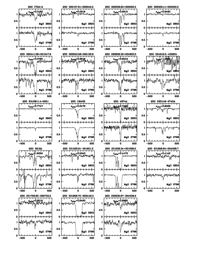
Figure 3: Selected Mg II absorption line systems in each of the 19 spectra comprising the high-resolution sample, S1. Each panel (normalized flux vs. rest-frame velocity in km s^-1) shows the strongest Mg II doublet in the spectrum, unless an absorption redshift is within [$z_{\rm min},z_{\rm max}$] of a cluster in the same LOS, in which case that latter system is plotted. Associated systems ($z_{\rm abs}\sim z_{\rm em}$) were not considered

References

- (1) Barkhouse, W. A., Green, P. J., Vikhlinin, A., et al. 2006, ApJ, 645, 955
- (2) Bartelmann, M., & Loeb, A. 1996, ApJ, 457, 529
- (3) Bergeron, J., & Stasinska, G. 1986, A&A, 169, 1
- (4) Bergeron, J., & Boissé, P. 1991, A&A, 243, 344
- (5) Bouche, N., Murphy, M. T., Peroux, C., Csabai, I., & Wild, V. 2006, MNRAS, 371, 495 (BMPCW06)
- (6) Boyle, B. J., Fong, R., & Shanks, T. 1988, MNRAS, 231, 897
- (7) Bravo-Alfaro, H., Cayatte, V., van Gorkom, J. H., & Balkowski, C. 2000, AJ, 119, 580
- (8) Butcher, H. & Oemler, G. 1984, ApJ, 285, 426
- (9) Caulet, A. 1989, ApJ, 340, 90
- (10) Chung, A., van Gorkom, J. H., Kenney, J. D. P. & Vollmer, B. 2007, ApJ, 659, 115
- (11) Churchill, C. W., Rigby, J. R., Charlton, J. C., & Vogt, S. S. 1999, ApJS, 120, 51 (CRCV99)
- (12) Churchill, C.W., Mellon, R.R., Charlton, J.C., Jannuzi, B.T., Kirhakos, S., Steidel, C.C., & Schneider, D.P. 2000, ApJ, 543, 577
- (13) Churchill, C. W., Vogt, S. S., & Charlton, J. C. 2003, ApJ, 125, 98
- (14) Churchill et al. 2005, IAU Conference 199, Shangai
- (15) Churchill, C. W., Kacprzak, G. G., Steidel, C. C., & Evans, J. L. 2007, ApJ, arXiv:astro-ph/0612560
- (16) Cooke, J., Wolfe, A. M., Gawiser, E. & Prochaska, J. X. 2006, ApJ, 636, 9
- (17) Cooray, A, 2006, MNRAS, 365, 842
- (18) Croton, D., et al., 2006, MNRAS, 365, 11
- (19) Dressler, A. 1980, ApJ, 236, 351
- (20) Ellison, S. L. & Lopez, S., 2001, A& A, 380, 117
- (21) Ellison, S. L., Yan, L., Hook, I. M., Pettini, M., Wall, J. V. & Shaver, P. 2002, A&A 383, 91
- (22) Ellison, S. L., Churchill, C. W., Rix, S. A., & Pettini, M. 2004a, ApJ, 615, 118
- (23) Ellison, S. L., Ibata, R., Pettini, M., Lewis, G. F., Aracil, B., Petitjean, P. & Srianand, R. 2004b A&A, 414, 79
- (24) Ellison, S. L., Kewley, L. J., & Mallén-Ornelas, G., 2005, MNRAS, 357, 354
- (25) Ellison S. L., 2006, MNRAS, 368, 335
- (26) Ettori, S. 2003, MNRAS, 344, L13
- (27) Fassnacht, C. D., et al. 2006, ApJ, 651, 667
- (28) Faure, C., Alloin, D., Kneib, J. P., & Courbin, F., 2004, A&A, 428, 741
- (29) Gehrels, N., 1986, ApJ, 303, 336
- (30) Gilbank, D., Yee, H. K. C., Ellingson, E., Gladders, M. D., Barrientos, L. F. & Blindert, K. 2007, AJ, 134, 282
- (31) Giovanelli, R. & Haynes, M. P. 1983, AJ, 88, 881
- (32) Gladders, M. D., Yee, H. K. C., Majumdar, S., Barrientos, L. F., Hoekstra, H., Hall, P. B., & Infante, L. 2007, ApJ, 655, 128
- Gladders & Yee (2005) Gladders, M. D., & Yee, H. K. C. 2005, ApJS, 157, 1
- Gladders & Yee (2000) Gladders, M. D., & Yee, H. K. C. 2000, AJ, 120, 2148
- (35) Green, P. J., Infante, L., Lopez, S., Aldcroft, T. L., & Winn, J. N. 2005, ApJ, 630, 142
- (36) Kacprzak, G. G., Churchill, C. W., Steidel, C. C., Murphy, M. T., & Evans, J. L. 2007, ApJ, 662, 909
- (37) Kneib, J.-P., Cohen, J. G., & Hjorth, J. 2000, ApJ, 544, L35
- (38) Koester, B. P. et al. 2007, ApJ, 660, 239
- (39) Lanzetta, K.M., Turnshek, D.A., & Wolfe, A.M. 1987, ApJ, 322, 739
- (40) Lanzetta, K.M., & Bowen, D. 1990, ApJ, 357, 321
- (41) Le Brun, V., Bergeron, J., Boisse, P., & Deharveng, J. M. 2001, A&A, 321, 733
- (42) Lopez, S. & Ellison, S. L., 2003, A& A, 403, 573
- (43) Lynch, R. S., Charlton, J. C., & Kim, T. S. 2006, ApJ, 640, 81
- (44) Maller A. H. & Bullock J. S., 2004, MNRAS, 355, 694 McCarthy, I. G., Bower, R. G., & Balogh, M. L. 2007, MNRAS, arXiv:astro-ph/0609314
- (45) Ménard, B., Nestor, D., Turnshek, D., Quider, A., Richards, G., Chelouche, D., & Rao, S. 2007, ApJ (arXiv:0706.0898)
- (46) Miller, E. D., Bregman, J. N., & Knezek, P. M. 2002, ApJ, 569, 134
- (47) Myers, A. D., Outram, P. J., Shanks, T., Boyle, B. J., Croom, S. M., Loaring, N. S., Miller, L., & Smith, R. J. 2003, MNRAS, 342, 467
- (48) Narayanan, A., Misawa, T., Charlton, J. C. & Kim, T.-S. 2007, ApJ, 660, 1093
- (49) Navarro, J. F., Frenk, C. S., & White, S. D. M. 1997, ApJ, 490, 493
- (50) Nestor, D. B., Turnshek, D. A., & Rao, S. M. 2005, ApJ, 628, 637 (NTR05)
- (51) Nestor, D. B., Turnshek, D. A., & Rao, S. M. 2006, ApJ, 643, 75 (NTR06)
- (52) Nestor, D. B., Turnshek, D. A., Rao, S. M. & Quider, A. M., 2007, ApJ, 658, 185
- (53) Perlman, E. S.. Horner, D. J., Jones, L. R., Scharf, C. A., Ebeling, H., Wegner, G., & Malkan, M. 2002, ApJS, 140, 265
- (54) Petitjean P., & Bergeron J., 1990, A&A, 231, 309
- (55) Pisano, D. J., Barnes, D. G., Gibson, B. K., Staveley-Smith, L., Freeman, K., & Kilborn, V. A., 2007, ApJ (arXiv:astro-ph/0703279)
- (56) Prochaska, J. X., & Herbert-Fort, S. 2004, PASP, 116, 622
- (57) Prochaska, J. X., Hennawi, J. F. & Herbert-Fort, S. 2007, arXiv:astro-ph/0703594
- (58) Prochter, G. E., Prochaska, J. X., & Burles, S. M. 2006, ApJ, 639, 766 (PPB06)
- (59) Rao, S.M., & Turnshek, D.A. 2000, ApJS, 130, 1
- (60) Rao, S. M., Turnshek, D. A., & Nestor, D. B. 2006, ApJ, 636, 610
- (61) Rigby, J. R., Charlton, J. C., & Churchill, C. W. 2002, ApJ, 565, 743
- (62) Russell, D. M., Ellison, S. L. & Benn, C. R. 2006, MNRAS, 367, 412
- (63) Schneider, D. P. et al. 2005, AJ, 130, 367
- (64) Scranton, R., et al. 2005, ApJ, 633, 589
- (65) Smette, A, Claeskens J.-F.& Surdej, J. 1997, New Astronomy, 2, 53
- (66) Sparks, W. B., Carollo, C. M., & Macchetto, F. 1997, ApJ, 486, 253
- (67) Spergel, D. N., Bean, R., Dore , O., Nolta, M. R., Bennett, C. L., Hinshaw, G., Jarosik, N., Komatsu, E., Page, L., Peiris, L., Verde, L., Barnes, C., Halpern, M., Hill, R. S., Kogut, A., Limon, M., Meyer, S. S., Odegard, N., Tucker, G. S., Weiland, J. L., Wollack, E., & Wright, E. L. 2007, arXiv:astro-ph/0603449
- (68) Steidel, C. C., Kollmeier, J. A., Shapley, A. E., Churchill, C. W., Dickinson, M., & Pettini, M., 2002, ApJ, 570, 526
- (69) Steidel, C. C., & Sargent, W. L. W. 1992, ApJS, 80, 1
- (70) Stocke, J. T., Morris, S. L., Gioia, I. M., Maccacaro, T., Schild, R., Wolter, A., Fleming, T. A., & Henry, J. P. 1991, ApJS, 76, 813
- (71) Takei, Y., Henry, J. P., Finoguenov, A., Mitsuda, K., Tamura, T., Fujimoto, R., & Briel, U. G., 2007, ApJ, 655, 831
- (72) Tytler, D., Boksenberg, A., Sargent, W.L.W., Young, P., & Kunth, D. 1987, ApJS, 64, 667
- (73) Verheijen, M., van Gorkom, J., Szomoru, A., Dwarakanath, K. S., Poggianti, B., & Schiminovich, D., 2007, NewAR, 51, 90
- (74) Vollmer, B., Soida, M., Beck, R., Urbanik, M., Chyży, K. T., Otmianowska-Mazur, K., Kenney, J. D. P., & van Gorkom, J. H. 2007, A&A 464, 37
- (75) Vollmer, B., Braine, J. Combes, F., & Sofue, Y. 2005, A&A 441, 473
- (76) White S. D. M., Navarro J. F., Evrard A. E., & Frenk C. S. 1993, Nature, 366, 429
- (77) Williger, G. M., Campusano, L. E., Clowes, R. G. & Graham, M. J. 2002, ApJ, 578, 708
- (78) Wolfe, A. M., Howk, J. C., Gawiser, E., Prochaska, J. X., & Lopez, S. 2004, ApJ, 615, 625
- Yee & Ellingson (2003) Yee, H. K. C., & Ellingson, E. 2003, ApJ, 585, 215
- (80) York et al. 2000, AJ, 120, 1579
- (81) Zibetti, S. Ménard, B., Nestor, D. B., Quider, A. M., Rao, S. M., & Turnshek, D. A. 2007, ApJ, 658, 161
- (82) Zwaan M. A., et al. 2003, AJ, 125, 2842