The thermonuclear rate for the ¹⁹F($\alpha$,p)²²Ne reaction at stellar temperatures

Abstract

The ¹⁹F($\alpha$,p)²²Ne reaction is considered to be one of the main sources of fluorine depletion in AGB and Wolf-Rayet stars. The reaction rate still retains large uncertainties due to the lack of experimental studies available. In this work the yields for both exit channels to the ground state and first excited state of ²²Ne have been measured and several previously unobserved resonances have been found in the energy range E_lab=792-1993 keV. The level parameters have been determined through a detailed R-matrix analysis of the reaction data and a new reaction rate is provided on the basis of the available experimental information.

I Introduction

Fluorine is by far the least abundant of the elements with atomic mass between 11 and 32. While several nucleosynthesis scenarios have been proposed for the production of fluorine, a unique site for the origin of this element has not been identified yet.

Presently three different scenarios are being discussed for the origin of fluorine. One possible process is the neutrino dissociation of ²⁰Ne in supernovae type II Woosley and Haxton (1988). A second scenario is the pulsating He-burning stage in AGB stars Busso (2006) and the third possibility is the hydrostatic burning of helium in Wolf-Rayet stars Goriely et al. (1989). It may be possible that all three sites contribute to the formation of fluorine in the universe Renda et al. (2004). So far, the only extra solar system objects in the galaxy where fluorine has been observed are AGB stars Jorrisen et al. (1992) and post-AGB star configurations Werner et al. (2005).

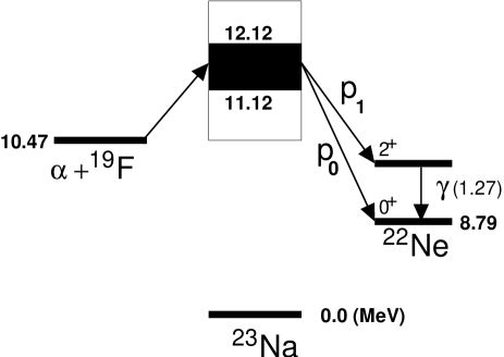
Figure 1: Energy level scheme for the ¹⁹F($\alpha$,p)²²Ne reaction. The entrance channel ($\alpha+^{19}$F) has a threshold of 10.47 MeV with respect to the ground state of ²³Na. The compound state can decay either via the p₀ channel to the ground state of ²²Ne or by the p₁ channel to the first excited state of ²²Ne. The subsequent emission of a 1.27 MeV photon from the decay of the first excited state (2⁺) to the ground state (0⁺) of ²²Ne can also be observed. The dark rectangle above ²³Na represents the energy region studied in this work. White regions above and below it correspond to energies where the cross sections were extrapolated.

Fluorine nucleosynthesis in AGB stars takes place in the hydrogen-helium intershell region where the ¹⁴N ashes from the preceding CNO burning are converted to ¹⁸F by $\alpha$-particle captures (a similar reaction path is followed by Wolf-Rayet stars). The unstable ¹⁸F isotope decays with a half life of 109.8 minutes to ¹⁸O. Both a proton or an $\alpha$-particle can be captured by ¹⁸O. In the former case, ⁴He and ¹⁵N are being produced, while in the latter case ²²Ne is formed. This second possibility does not produce fluorine. The alternative ¹⁸O(p,$\alpha$)¹⁵N($\alpha,\gamma$)¹⁹F capture reaction is the main fluorine production link in this scenario. The abundance of ¹⁵N depends sensitively on the hydrogen abundance in the inter-shell region. Hydrogen has been depleted in the preceding CNO burning but can be regenerated through the ¹⁴N(n,p)¹⁴C reaction, with the neutrons being produced by the ¹³C($\alpha$,n)¹⁶O reaction. Additional protons may be mixed into the region when the convective envelope penetrates the intershell region at the end of the third dredge up (TDU). ¹⁴C produced by this reaction provides a second link for the production of ¹⁸O via ¹⁴C($\alpha,\gamma$)¹⁸O.

Fluorine is very fragile and three reactions may cause rapid fluorine destruction. Because of the high abundance of ⁴He in the intershell region, the ¹⁹F($\alpha$,p)²²Ne is expected to be a dominant depletion link. Another depletion process corresponds to the ¹⁹F(n,$\gamma$)²⁰F reaction, caused by neutrons being produced by the ¹³C($\alpha$,n)¹⁶O or the ²²Ne($\alpha$,n)²⁵Mg reactions. If hydrogen is available in sufficient abundance, fluorine may also be depleted through the very strong ¹⁹F(p,$\alpha$)¹⁶O reaction. All this, however, is strongly correlated with the existing proton and $\alpha$-particle abundance at the fluorine synthesis site.

The reaction rate for ¹⁹F($\alpha$,p)²²Ne is highly uncertain at helium burning temperatures. Even recent nucleosynthesis simulations Palacios et al. (2005) still rely on the very simplified rate expression of Caughlan and Fowler (CF88) Caughlan and Fowler (1988) based on an optical model approximation for estimating the cross section of compound nuclear reactions with overlapping resonances. This approach was originally developed Fowler and Hoyle (1964) and employed Wagoner (1969); Fowler et al. (1975) for cases where no experimental information was available. This reaction rate is in reasonable agreement with more recent Hauser-Feshbach estimates assuming a high density of unbound states in ²³Na Thielemann et al. (1986). Other ¹⁹F nucleosynthesis simulations Lugaro et al. (2004); Stancliffe et al. (2005) rely on the sparse experimental data available for ¹⁹F($\alpha$,p)²²Ne for E_lab=1.3 MeV to 3.0 MeV Kuperus (1965), estimating also possible low energy resonant contributions from known $\alpha$-particle unbound states in ²³Na Endt (1990). For example, in their approach they approximated the reaction rate by only considering the resonance contributions of the various states neglecting possible interference effects and broad-resonance tail contributions. In this paper we describe a new measurement of ¹⁹F($\alpha$,p)²²Ne at lower energies. In our study we explored the reaction for E_lab=792 to 1993 keV at different angles. The pronounced resonance structure was analyzed in terms of the multi-channel R-matrix model using the recently developed R-matrix code AZURE Azuma (2005). Energy regions not measured here were also included in the computation of the stellar reaction rate by using a combination of data available in the literature and our experimental results to extrapolate the reaction cross section. Possible low energy resonances were taken into account sampling characteristic $\alpha$-particle partial widths of the known $\alpha$-particle unbound states in ²³Na, while deriving the corresponding proton partial width from the available elastic scattering data in the literature Keyworth et al. (1968). Interference terms were modelled with Monte Carlo simulations. In section 2 we describe the experimental setup and the experimental procedure. The R-matrix analysis of the experimental data and the determination of the nuclear parameters of resonances is described in section 3. Finally, the experimental and extrapolated reaction rates (with error bars) are presented and discussed in section 4.

II Experimental Method

The destruction of ¹⁹F by an $\alpha$-particle capture occurs mainly by a resonant reaction process through the ²³Na compound nucleus in an excitation range of high level density. The populated resonant levels will decay by proton emission to the ground state (p₀) or first excited state (p₁) of ²²Ne. This study included the direct measurement of the ¹⁹F($\alpha$,p)²²Ne reaction by detecting both p₀ and p₁ protons (see Ugalde et al. (2005) and Ugalde (2005)) as well as the additional measurement of the p₁ channel via the detection of the $\gamma$-ray transition Ugalde et al. (2006) from the first excited state (2⁺) to the ground state (0⁺) of ²²Ne (see figure 1).

The experiment was performed at the Nuclear Science Laboratory of the University of Notre Dame using the 3.5 MV KN Van de Graaff accelerator. In a first run, the excitation curve of ¹⁹F($\alpha$,p)²²Ne was investigated between E_lab=1224 keV and 1993 keV. For this experiment two Si surface barrier detectors with a depletion depth of 300 $\mu$m were mounted at forward angles, while one 100 $\mu$m Si detector was positioned at a backward angle. These thicknesses were sufficient for stopping the reaction protons. The effective solid angle of the detectors at each position configuration was determined using a mixed ²⁴¹Am and ¹⁴⁸Gd $\alpha$-particle source with a known activity placed at the target position.

The energy range between E_lab=1629 keV to 1993 keV was mapped in 5 keV energy steps with the detectors mounted at 30^o, 90^o and 130^o. This made it possible to use the two known resonances at E_lab=1.67 MeV and 1.89 MeV Kuperus (1965) as reference for calibrating and matching the reaction yield to the previous results. At lower energies, the detector position was changed to 40^o, 100^o and 120^o with respect to the beam direction. The excitation curve was mapped from E_lab=1220 to 1679 keV using the E_lab=1.67 MeV resonance as a reference. In total 483 proton spectra were acquired and for every energy, one elastic scattering $\alpha$-particle spectrum was taken. The stoichiometry of targets was constantly monitored with back-scattered $\alpha$-particles.

The ¹⁹F transmission targets were prepared by evaporating 10 $\mu$g/cm² of CaF₂ on 40 $\mu$g/cm² natural carbon substrates, mounted on aluminum frames. The target was placed with the evaporated material facing the beam on a ladder attached to a rotating rod at the center of the scattering chamber. The ladder held one target and a collimator that was used for centering the beam. The targets deteriorated significantly under beam bombardment, so their stability was monitored by measuring frequently the yield of the elastically scattered $\alpha$-particles at the E_lab=1.89 MeV resonance. Targets were constantly replaced with new and recently evaporated targets.

For any two detectors with the same absolute efficiency the relative count rate is independent of target stoichiometry and beam intensity, as expressed by

$${N_{1}(E,\theta)\over N_{2}(E,\theta)}=\biggl{[}{d\Omega_{1}\over d\Omega_{2}}\biggl{]}_{lab\over cm}\biggl{(}{d\sigma(E,\theta)\over d\Omega}\biggl{)}_{2}^{-1}\biggl{(}{d\sigma(E,\theta)\over d\Omega}\biggl{)}_{1}.$$ (1)

$N_{1}(E,\theta)$ and $N_{2}(E,\theta)$ corresponds to the number of events in detectors 1 and 2, respectively, $\bigl{[}$$d\Omega_{1}\over d\Omega_{2}$$\bigl{]}$_lab/cm is the solid angle correcting for center of mass to the laboratory system, and $d\sigma(E,\theta)\over d\Omega$ are the differential cross sections measured at detectors 1 and 2, respectively. The differential cross section of the ¹⁹F($\alpha$,p)²²Ne reaction was determined relative to the differential cross section for elastic scattering measured at 160^o. It has been shown by Huang-sheng et al. Huan-sheng et al. (1994) and by Cseh et al. Cseh et al. (1984) that below E_lab=2.5 MeV the elastic scattering of ⁴He on ¹⁹F follows the Rutherford law,

$${d\sigma(E,\theta)\over d\Omega}_{el}={d\sigma(E,\theta)\over d\Omega}_{Ruth}=\biggl{(}{{Z_{1}Z_{2}e^{2}}\over{4E}}\biggl{)}^{2}\sin^{-4}{\theta\over 2}.$$ (2)

Z₁ and Z₂ are the atomic numbers of projectile and target, respectively, $e$ is the proton electric charge and e²=1440 keV fm, E is the relative energy of target and projectile in the center of mass system, and $\theta$ is the center of mass angle at which the elastically scattered particles are observed. Within the small thickness of the target (27$\pm$5 keV) the stopping cross section $\epsilon$ is assumed to be a constant. The variation of the elastic differential cross section across the target thickness is also very small. Therefore the elastic yield can be expressed as

$$Y_{elas}=\biggl{(}{d\sigma(E,\theta)\over d\Omega}\biggl{)}_{Ruth}{\Delta\over\epsilon}.$$ (3)

Subsequently the target integrated proton yield Y_p can be expressed relative to the elastic scattering cross sections as

$$Y_{p}={\Delta\over\epsilon}\biggl{(}{d\sigma(E,\theta)\over d\Omega}\biggl{)}_{prot}=\biggl{(}{N_{prot}(E,\theta)\over N_{elas}(E,\theta)}\biggl{)}\biggl{(}{d\Omega_{prot}\over d\Omega_{elas}}\biggl{)}_{lab/cm}{\Delta\over\epsilon}\biggl{(}{{Z_{1}Z_{2}e^{2}}\over{4E}}\biggl{)}^{2}\sin^{-4}{\theta\over 2}.$$ (4)

The energy dependence of the stopping power $dE/dx$ of ⁴He is well known for both calcium and fluorine Ziegler (1985). The stopping power for fluorine was fitted to a quadratic polynomial function given by

$$\biggl{(}{dE\over dx}\biggl{)}_{F}=\sum_{i=0}^{2}a_{i}E^{i}.$$ (5)

A similar relation was determined for the calcium stopping power. The partial stopping cross section $\epsilon$ for each of the nuclear species in the target is described by:

$$\epsilon={1\over n}\biggl{(}{dE\over dx}\biggl{)},$$ (6)

where

$$n=\nu\rho N_{A}/A$$ (7)

with $\nu$ the number of atoms per molecule, $\rho$ the density of the target (again assuming the evaporated material has the same density as the powder used before target preparation), $N_{A}$ the Avogadro number, and $A$ the mass number. The total stopping cross section of the calcium fluoride target depends critically on the target stoichiometry

$$\epsilon=\epsilon_{F}+{N_{Ca}\over N_{F}}\epsilon_{Ca}.$$ (8)

The ratio ${N_{Ca}\over N_{F}}$ measured in the evaporated target layer does not necessarily reflect the stoichiometry of the material before being evaporated. It was reported in previous work Lorenz-Wirzba (1978) that evaporated CaF₂ shows a stoichiometric calcium to fluorine ratio of 1:1. The targets used in the present experiment were tested using well known resonances in the ¹⁹F(p,$\alpha\gamma$)¹⁶O reaction. The results indicated that the stoichiometry of the evaporated material is the same as that of the CaF₂ powder Couture (2005).

In a second set of experiments we measured the proton yield at lower energies. The experimental setup was designed to perform the measurements with higher beam currents and larger detector solid angles to compensate for the drop in reaction cross section.

The target chamber for this set of experiments allowed mounting of the target at two different angles with respect to the beam: at 45^o and 90^o. With the first option we measured scattering angles below 90^o, while with the second other angles were measured at a smaller effective target thickness. We tested several ¹⁹F-implanted targets for stability. Substrates tested were Ta, Ni, Cr, Al, Fe, and Mo. The best stability against beam deterioration was obtained for the Fe substrate. Electron suppression was supplied through an aluminum plate at -400 volts, mounted 5 mm in front of the target. Carbon buildup on the target was minimized with a liquid nitrogen-cooled copper plate. The target itself was water cooled from the back and electrically isolated from the scattering chamber. Beam current was directly measured at the target holder.

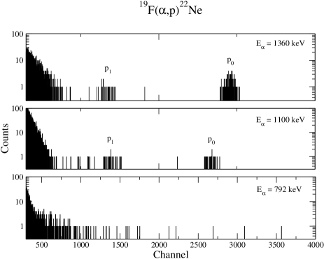
Figure 2: Proton spectra for ¹⁹F($\alpha$,p)²²Ne at 135^o for three beam energies (label at the right upper corner of each box). The upper spectrum shows both proton groups at the reference resonance. Both peaks appear clean of background and are easy to identify. The spectrum at E_lab=1100 keV shows two groups of protons, still well isolated from the background. Finally, a spectrum at E_lab=792 keV, where no proton groups were positively identified is shown. The integrated charges are (in $\mu$C) 1981, 180647, and 519252, respectively.

Two Si detectors were mounted on the rotating plate with aluminum holders. Collimators were placed in front of the detectors and pin hole-free Al foils were used to stop the elastically scattered $\alpha$-particles, while allowing the protons to reach the surface of the detectors. Both detector holders and the rotating plate were electrically isolated from the rest of the chamber. The detectors had an effective detection area of 450 mm². The solid angles for both detectors were determined using a mixed ²⁴¹Am+¹⁴⁸Gd $\alpha$-particle source of known activity mounted at the target position. We measured them to be 0.130$\pm$0.026 and 0.133$\pm$0.027 steradians, respectively.

With the chamber at the perpendicular target position and both detectors at 135^o, a total of 540 spectra were acquired for laboratory energies between 792 and 1380 keV. Typical spectra are shown in figure 2; the last spectrum taken (E_lab=792 keV) does not show identifiable proton groups. Subsequently, the chamber was reoriented to the 45^o target position. The detectors were mounted at 150^o and 120^o with respect to the beam direction and 178 spectra were taken. Finally, the detectors were mounted at 75^o and 105^o with respect to the beam direction and 69 spectra were measured.

In this experimental configuration the reaction yield could not be normalized to elastic scattering because of the thick target backing material. The yield was therefore measured relative to the accumulated charge on the target during each run. The reaction yield Y_p($\theta$) for the detector mounted at angle $\theta$ is derived from the number of registered proton events N_p($\theta$) in the detector is

$$Y_{p}(\theta)=\frac{N_{p}(\theta)}{N_{\alpha}\cdot\epsilon_{p}\cdot d\Omega_{p}},$$ (9)

where N_α is the accumulated charge, $\epsilon_{p}$ is the absolute detection efficiency (assumed to be 1 for charged particles and Si detectors at very low count rates), and $d\Omega_{p}$ is the solid angle subtended by the detector.

The differential cross section can be directly derived from the reaction yield normalized to the yield of the E_lab=1.37 MeV resonance as measured in the first experiment. This depends critically on the stability of the fluorine content in the target material. Since the amount of fluorine decreases with accumulated charge, the reaction yield needs to be corrected accordingly. During the experiment the yield of the E_lab=1.37 MeV resonance was monitored frequently to correct for target degradation. The on-resonance thick target yield Y_tt as a function of accumulated charge N_α can be expressed by the linear relation:

$$Y_{tt}=a+bN_{\alpha},$$ (10)

with a and b as constants. The measured yield of the observed protons Y_p(E) was corrected for target degradation in terms of the accumulated charge to

$$Y^{\prime}_{p}(E)=\frac{a}{a+bN_{\alpha}}\cdot Y_{p}(E).$$ (11)

Data obtained from all the described experiments consist of 20 excitation functions, with eleven corresponding to ¹⁹F($\alpha$,p₀)²²Ne and nine to ¹⁹F($\alpha$,p₁)²²Ne. Ten angles were measured in different energy regions. All add up to 1471 data points (See table 1) which were analyzed in terms of the R-matrix theory.

Table 1: Yield curves measured in this work

curve	channel	angle	Emin (keV)	Emax (keV)	$\Delta$ (keV)
1	${}^{19}F(\alpha,p_{0})^{22}Ne$	130	1641	1993	15
2	${}^{19}F(\alpha,p_{0})^{22}Ne$	90	1641	1993	15
3	${}^{19}F(\alpha,p_{0})^{22}Ne$	30	1641	1993	15
4	${}^{19}F(\alpha,p_{0})^{22}Ne$	120	1224	1679	15
5	${}^{19}F(\alpha,p_{0})^{22}Ne$	100	1224	1679	15
6	${}^{19}F(\alpha,p_{0})^{22}Ne$	40	1224	1679	15
7	${}^{19}F(\alpha,p_{0})^{22}Ne$	105	1027	1367	25
8	${}^{19}F(\alpha,p_{0})^{22}Ne$	120	929	1359	35
9	${}^{19}F(\alpha,p_{0})^{22}Ne$	135	792	1363	25
10	${}^{19}F(\alpha,p_{0})^{22}Ne$	150	929	1359	35
11	${}^{19}F(\alpha,p_{0})^{22}Ne$	75	1027	1367	35
12	${}^{19}F(\alpha,p_{1})^{22}Ne$	130	1629	1981	15
13	${}^{19}F(\alpha,p_{1})^{22}Ne$	90	1629	1981	15
14	${}^{19}F(\alpha,p_{1})^{22}Ne$	30	1629	1981	15
15	${}^{19}F(\alpha,p_{1})^{22}Ne$	120	1224	1679	15
16	${}^{19}F(\alpha,p_{1})^{22}Ne$	100	1224	1679	15
17	${}^{19}F(\alpha,p_{1})^{22}Ne$	40	1224	1679	15
18	${}^{19}F(\alpha,p_{1})^{22}Ne$	120	929	1359	35
19	${}^{19}F(\alpha,p_{1})^{22}Ne$	135	792	1363	25
20	${}^{19}F(\alpha,p_{1})^{22}Ne$	150	929	1359	35

III Multichannel R-matrix analysis

For the analysis of the experimental data we used the A-matrix version of the computer code AZURE Azuma (2005). AZURE is a multichannel and multilevel code that implements the A- and R-matrix formalisms as presented by Lane and Thomas Lane and Thomas (1958). The code is capable of fitting experimental datasets by varying formal parameters (energies and width amplitudes) of compound-nucleus states. The integrated cross section can also be computed from angular distribution datasets. Error bars for both the parameters and cross section curves are treated with Monte Carlo techniques.

The input to the code consists of a set of initial nuclear parameters; each level is characterized by one energy eigenvalue and several formal reduced width amplitudes (one per channel per level). The code identifies open reaction channels and from the input it assigns an independent width amplitude for each (s,l) combination allowed for the level. Theoretical differential cross section curves at different angles are computed and then compared to experimental yields after target integration corrections Ugalde (2006). The maximum likelihood estimator is then minimized by varying all the parameters simultaneously. Each time a local minimum is found, the integrated value of the cross section is computed.

Overlapping of resonances complicated the simultaneous fitting of the yield curves. The code was by itself not able to find a set of formal parameters that would reasonably describe the yield curves. For this reason, an initial parameter set had to be found without the help of the minimization routines. By trial and error, the choice of initial nuclear parameters was done by adjusting the energy for each of the levels so as to describe the position of resonances as close as possible. The height and width of the resonances was, on the other hand, approximated by varying the width amplitudes.

Interference patterns between the various resonances were determined by iteratively probing the contribution to yield curves of levels within groups of the same J^π. The sign of the width amplitudes was flipped one by one for all the (s,l) channels. These steps were repeated iteratively several times until the theoretical curves resembled the dataset. The resulting set of parameters was then used as input to the R-matrix code coupled to the $\chi^{2}$ minimization routines. Every time a calculation was performed all 20 excitation curves were examined. The target thickness $\Delta$ used for each of the yield curves is shown in table 1.

Figure 3: Experimental yield curves for the ¹⁹F($\alpha$,p₀)²²Ne channel and the R-matrix fits (solid lines). Different curves are offset by a factor of 100. Vertical axis units are relative yields. The labels to the right of each curve are described in table 1.

Figure 4: Experimental yield curves for the ¹⁹F($\alpha$,p₁)²²Ne channel and the R-matrix fits (solid lines). Different curves are offset by a factor of 100. Vertical axis units are relative yields. The labels to the right of each curve are described in table 1.

The resulting R-matrix fits to the experimental yield data $Y_{p}$ are shown in figures 3 and 4 for the ground state and the excited state transitions, respectively. Both the energies E_λ and reduced width amplitudes $\gamma_{i}$ were determined with a single channel radius (a_c=5.5 fm). The boundary condition was set to $S_{c}$, the shift function, at the level in each J^π group with the lowest energy. Background states were included for each of the J^π groups. (The set of 201 R-matrix parameters and the experimental dataset can be obtained by contacting the author.)

Parameter error bars were determined with a bootstrap method Press et al. (1992) and correspond to a confidence interval of 95% (see figure 5). From the set of 1,471 experimental data points we generated 40,000 subsets, with each subset containing 1,471 data points as well. The selection of points was performed with a Monte Carlo method and as a result, each set contains a random number of points repeated more than once. Using the set of formal parameters obtained with the R-matrix analysis described above, a $\chi^{2}$ was computed for each of the subsets sampled by bootstrapping. The distribution of $\chi^{2}$ values is shown in figure 5(a). The 0.95 cumulative value of the distribution corresponds to $\chi^{2}\equiv\chi^{2}_{95}$=22,774. Finally, with a Monte Carlo technique, we generated $\chi^{2}$ curves by varing each parameter independently while fixing all others. The error bar corresponds to the largest parameter value such that $\chi^{2}$ $\leq$ $\chi^{2}_{95}$ (see figure 5(b)). Total cross sections for both channels were computed as well and are discussed in the next section and shown in figure 6.

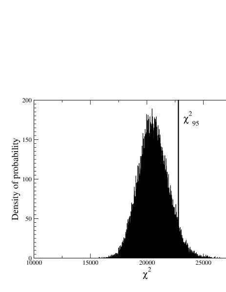
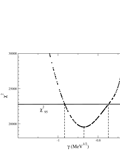
Figure 5: Calculation of error bars. (a) Bootstrap histogram used to compute the error bars with a 95% confidence level. The horizontal axis corresponds to the raw $\chi^{2}$ value associated to the set of central-value parameters. Each bin contains intervals $\Delta\chi^{2}$=20. A total of 40,000 subsets were sampled from the experimental set with a Monte Carlo method. Note that the curve does not correspond to a normal distribution. However, the centroid corresponds to the raw value of $\chi^{2}$ associated to the best R-matrix fit ($\chi^{2}_{min}$=20,535). An area corresponding to 95% of the total integral is below $\chi^{2}_{95}$=22,774 (vertical line). (b) Sample $\chi^{2}$ vs. parameter value ($\gamma$) curve. The horizontal line represents $\chi^{2}_{95}$, while the dotted vertical lines are, from left to right, the lower limit, central value, and upper limit of the parameter, respectively. An equivalent curve was generated for each of the formal parameters.

IV The reaction rate

The thermonuclear reaction rate has contributions from three energy regimes: a) the region measured experimentally in this work, spanning from E_lab=792 keV to 1993 keV, b) the region below E_lab=792 keV (not measured), and c) the region above E_lab=1993 keV (not measured here as well).

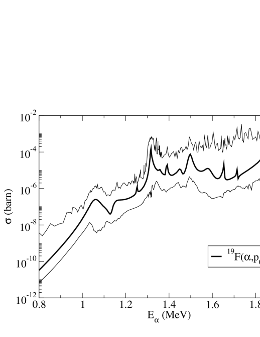
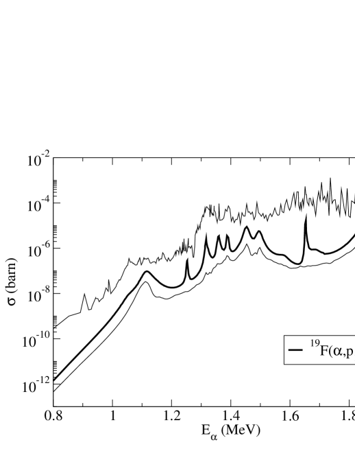
Figure 6: R-matrix calculated total cross sections for ¹⁹F($\alpha$, p)²²Ne. Both ¹⁹F($\alpha$, p₀)²²Ne (upper panel) and ¹⁹F($\alpha$, p₁)²²Ne (lower panel) curves are shown with uncertainty bands, as computed by sampling the 95% confidence interval nuclear parameter space with a Monte Carlo method. The strong oscillations in the upper and lower limits of the bands are an artifact of the finite number of samples (10,000) taken with the Monte Carlo method.

The contribution to the rate from our experimental dataset was calculated by integrating numerically the total cross section $\sigma(E)$ over the Maxwell-Boltzmann distribution of stellar gas at temperature $T$

$${N_{A}}\langle\sigma v\rangle={N_{A}}{\biggl{(}{8\over{\pi\mu}}\biggl{)}^{1/2}{(kT)^{-3/2}}{\int\sigma(E)E\exp\biggl{(}{{-E}\over{kT}}\biggl{)}dE}}.$$ (12)

Here E is the energy of the particles in the center of mass system, N_A is Avogadro’s number, k is Boltzmann’s constant, $\mu$ the reduced mass, and T the temperature of the gas. The total cross section $\sigma$ was derived from the R-matrix calculation with the recommended values of formal parameters. Both p₀ and p₁ components are shown in figure 6. Upper and lower limits of the total cross section and the reaction rate in this energy regime were computed by sampling the parameter space defined by the upper and lower values of the fitting parameters with a Monte Carlo technique. All parameters were varied simultaneously and a total of 10,000 parameter sets were produced. The reaction rate for each parameter set was calculated with equation 12 and all resulting rates were compared with each other. The highest (lowest) value obtained corresponds to the upper (lower) limit of the reaction rate.

The contribution to the reaction rate from resonances below E_lab=792 keV, which were not measured in the present experiment, was considered as well. Previous studies through other reaction channels do indicate several unbound states in ²³Na in this energy range near the $\alpha$-particle threshold Endt (1990), which may contribute significantly to the ¹⁹F($\alpha$,p)²²Ne reaction. Most notably, detailed elastic proton scattering measurements were performed for this energy range in ²³Na Keyworth et al. (1968), and provide important information necessary for estimating the contributions of these lower energy states to the reaction rate. Resonances observed in the ²²Ne(p,p)²²Ne and ²²Ne(p,p’)²²Ne channels were used to define the spins, parities, energies, and both proton p₀ and p₁ partial widths of contributing states. On the other hand, $\alpha$-particle partial widths $\Gamma_{\alpha}$ were obtained by adopting the experimentally known $\alpha$-particle reduced widths $\gamma^{2}_{\alpha}$ determined in the high energy range.

Energies and reduced widths obtained with the R-matrix analysis were used to calculate the logaritmic average $<log(\gamma^{2}_{\alpha})>$ for each J^π group (see figure 7). The extrapolated reduced $\alpha$-particle width amplitude for a state with parameters (J,$\pi$) was chosen to be

$$\gamma^{2}_{\alpha}(J,\pi)=10^{<log(\gamma^{2}_{\alpha})>}.$$ (13)

Extrapolated upper (lower) limit values of the reduced $\alpha$-particle widths were set equal to the highest (lowest) $\gamma_{\alpha}^{2}$ value determined from the experimental data of the corresponding J^π group. The set of extrapolated $\gamma^{2}_{\alpha}$ values, together with the reduced proton widths $\gamma^{2}_{p}$ calculated from ²²Ne(p,p)²²Ne and ²²Ne(p,p’)²²Ne experiments by $\Gamma_{p}=2P\gamma^{2}_{p}$ (where $P$ is the penetrability through the Coulomb barrier) is shown in table 2.

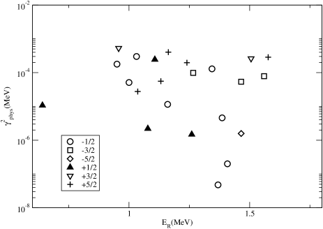
Figure 7: The experimentally determined $\gamma_{\alpha}^{2}$ as a function of center-of-mass energy, presented in sets of $J^{\pi}$.

Table 2: Nuclear parameters for states with E${}_{lab}<$792 keV.

$J$	$\pi$	$E_{cm}$ $(MeV)$	$\gamma^{2}_{\alpha}$ $(MeV)$	$\gamma^{2}_{\alpha}$ $(MeV)$	$\gamma^{2}_{\alpha}$ $(MeV)$
			Recomm	Upper	Lower
1.5	1	0.010	3.72E-4	5.29E-4	2.61E-4
1.5	-1	0.031	8.89E-5	1.51E-4	5.37E-5
0.5	1	0.037	9.60E-6	2.44E-4	1.48E-6
2.5	1	0.049	1.04E-4	4.04E-4	2.75E-5
2.5	1	0.078	1.04E-4	4.04E-4	2.75E-5
1.5	-1	0.106	8.89E-5	1.51E-4	5.37E-5
1.5	1	0.147	3.72E-4	5.29E-4	2.61E-4
2.5	1	0.147	1.04E-4	4.04E-4	2.75E-5
1.5	-1	0.207	8.89E-5	1.51E-4	5.37E-5
1.5	-1	0.237	8.89E-5	1.51E-4	5.37E-5
1.5	1	0.354	3.72E-4	5.29E-4	2.61E-4
1.5	-1	0.355	8.89E-5	1.51E-4	5.37E-5
1.5	1	0.369	3.72E-4	5.29E-4	2.75E-5
2.5	1	0.369	1.04E-4	4.04E-4	2.61E-4
1.5	-1	0.405	8.89E-5	1.51E-4	5.37E-5
0.5	-1	0.438	1.07E-5	3.00E-4	4.76E-8
2.5	1	0.438	1.04E-4	4.04E-4	2.75E-5
0.5	1	0.448	9.60E-6	2.44E-4	1.48E-6
1.5	1	0.461	3.72E-4	5.29E-4	2.61E-4
0.5	1	0.481	9.60E-6	2.44E-4	1.48E-6
2.5	1	0.503	1.04E-4	4.04E-4	2.75E-5
1.5	1	0.503	3.72E-4	5.29E-4	2.61E-4
1.5	1	0.506	3.72E-4	5.29E-4	2.61E-4
1.5	-1	0.511	8.89E-5	1.51E-4	5.37E-5
0.5	1	0.524	9.60E-6	2.44E-4	1.48E-6
1.5	1	0.525	3.72E-4	5.29E-4	2.61E-4
0.5	1	0.569	9.60E-6	2.44E-4	1.48E-6
0.5	-1	0.618	1.07E-5	3.00E-4	4.76E-8
2.5	1	0.640	1.04E-4	4.04E-4	2.75E-5
1.5	1	0.642	3.72E-4	5.29E-4	2.61E-4

Based on these parameters, the resonant contribution to the cross section was calculated using the R-matrix formalism. Nevertheless, the interference pattern between resonances can not be predicted in this scheme. Therefore, we simulated its effect with a Monte Carlo sampling of possible width amplitude sign combinations. Figure 8 shows the resulting S-factor for three sample assumptions for interference between resonances. Upper and lower values of the reaction rate were calculated with equation 12 from different combinations of signs and widths sampled within the parameter space, as before. The recommended value corresponds to the logaritmic average of the upper and lower limits of the reaction rate.

Finally, the contribution to the reaction rate from resonances above E_lab=1993 keV was computed by extrapolating our experimental rate to higher temperatures by following the energy dependence of the Hauser-Feshbach rate MOST Goriely (1998). We did not perform an R-matrix analysis due to the current uncertainty of spins and parities of excited states in ²³Na in this energy region, for which several experimental works have been published (for example see Cseh et al. (1984); van der Zwan and Geiger (1977); Schier et al. (1976); Kuperus (1965) ). Over one hundred resonances have been identified for 2.0 $\leq$ E_lab (MeV) $\leq$ 4.7, but the data has not been able to constrain the spins and parities of most of the states. The average level density is  0.04 keV^-1, high enough to apply the Hauser-Feshbach formalism for calculating the reaction rate Rauscher et al. (1997). At the upper limit of the Gamow window corresponding to our experimental data (T=1$\times$10⁹ K), the agreement between the Hauser-Feshbach and our R-matrix calculated rate is very good. We used the experimentally determined reaction rate here to renormalize the MOST values above this temperature.

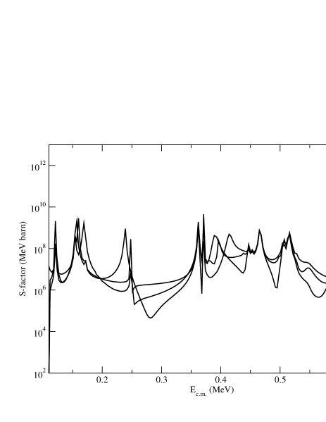
Figure 8: Monte Carlo simulated low energy S-factor for ¹⁹F($\alpha,p$)²²Ne for three different sample resonance interference assumptions.

The total reaction rate consists, for temperatures below T=1$\times$10⁹ K, of the sum of the rate from the R-matrix analysis of our experimental data and the rate calculated from extrapolated Monte Carlo cross sections at the lowest energies, and of the Hauser-Feshbach renormalized rate above T=1$\times$10⁹ K. The resulting reaction rate is shown in table 3.

Table 3: Reaction rate for ${}^{19}{F}(\alpha,p)^{22}{Ne}$

$T_{9}$	$N_{A}<\sigma v>$ recomm	$N_{A}<\sigma v>$ low	$N_{A}<\sigma v>$ up
	$[cm^{3}/s$ $mol]$	$[cm^{3}/s$ $mol]$	$[cm^{3}/s$ $mol]$
0.10	2.402E-22	1.049E-23	5.500E-21
0.11	5.072E-21	4.173E-22	6.166E-20
0.12	6.322E-20	8.649E-21	4.621E-19
0.13	5.625E-19	1.158E-19	2.732E-18
0.14	3.943E-18	1.117E-18	1.392E-17
0.15	2.477E-17	8.120E-18	7.555E-17
0.16	1.399E-16	4.807E-17	4.070E-16
0.18	2.758E-15	1.073E-15	7.091E-15
0.20	3.310E-14	1.455E-14	7.556E-14
0.25	3.680E-12	2.047E-12	7.088E-12
0.30	1.272E-10	7.709E-11	2.759E-10
0.35	2.431E-09	1.484E-09	6.038E-09
0.40	3.340E-08	1.939E-08	7.961E-08
0.45	3.631E-07	2.064E-07	7.438E-07
0.50	3.072E-06	1.796E-06	5.475E-06
0.60	1.020E-04	6.176E-05	1.601E-04
0.70	1.445E-03	8.658E-04	2.151E-03
0.80	1.115E-02	6.630E-03	1.624E-02
0.90	5.615E-02	3.346E-02	8.186E-02
1.00	4.173E-01	2.483E-01	6.068E-01
1.25	5.748E+00	3.398E+00	8.746E+00
1.50	3.946E+01	2.278E+01	6.111E+01
1.75	1.770E+02	1.007E+02	2.738E+02
2.00	5.944E+02	3.381E+02	9.115E+02
2.50	3.773E+03	2.169E+03	5.674E+03
3.00	1.456E+04	8.458E+03	2.160E+04
3.50	4.089E+04	2.394E+04	6.023E+04
4.00	9.261E+04	5.448E+04	1.359E+05
5.00	3.123E+05	1.846E+05	4.563E+05
6.00	7.420E+05	4.398E+05	1.082E+06
7.00	1.427E+06	8.467E+05	2.078E+06
8.00	2.393E+06	1.421E+06	3.484E+06
9.00	3.661E+06	2.175E+06	5.328E+06
10.00	5.253E+06	3.122E+06	7.643E+06

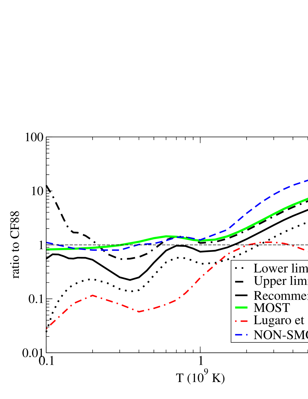
Figure 9: (Color figure) The new rate for the ¹⁹F($\alpha$,p)²²Ne reaction compared to the phenomenological rate listed in the literature (CF88) Caughlan and Fowler (1988), the Hauser-Feshbach predictions, and Lugaro et al.’s Lugaro et al. (2004) rate.

Figure 9 shows the total reaction rate relative to the phenomenological rate estimate of CF88. Shown are the Hauser-Feshbach model predictions using the codes MOST and NON-SMOKER relative to the CF88 predictions. Also compared is the rate estimate of Lugaro et al. Lugaro et al. (2004), which is based on a single non-interfering resonance approximation.

The new rate is significantly higher (about one order of magnitude in the stellar temperature regime) than the rate based on the assumption of single non-interfering resonance levels of Lugaro et al. Lugaro et al. (2004). This can be attributed to the fact that the new rate is calculated from non-narrow resonance contributions, as given by the R-matrix analysis. Also, the CF88 rate is very similar to the new rate, except for the astrophysically relevant temperature T = 3$\times$10⁸ K, where it is close to a factor of 10 smaller. However, the statistical model predictions overestimate the reaction rate and can be rejected at a 95% confidence level for 2.5 $<$ T (10⁸ K) $<$ 5.5. For the highest temperatures, the new recommended rate differs from the statistical model predictions by a renormalization factor (0.62).

The main source of uncertainty in the new rate at AGB star temperatures comes from the uncertainty in the extrapolation of the reaction cross section. Experimental work below E_lab=800 keV is required to constrain the partial $\alpha$-particle widths and the interference patterns in the ¹⁹F($\alpha$,p)²²Ne reaction. We have shown the importance of the interference effects between resonances. Therefore, a direct measurement towards lower energies is probably the only plausible solution to the problem of the uncertainty of this reaction rate at AGB star temperatures.

For explosive stellar scenarios (T $>$ 1$\times$10⁹ K ) the situation is still more delicate as spins and parities of resonances contributing to the rate are uncertain. Both direct and indirect measurements of the ¹⁹F($\alpha$,p)²²Ne reaction above E_lab=2 MeV can help improving the quality of the rate for explosive scenarios.

V Summary and conclusions

We have measured the ¹⁹F($\alpha$,p)²²Ne reaction in the energy range $E_{lab}$=792-1993 keV. Stable fluorine targets were developed and several resonances were found in the 20 experimental yield curves. Ten different angles ranging from 30^o to 150^o were measured and two reaction channels ($p_{0}$ and $p_{1}$) observed. An R-matrix analysis of the data was performed to determine the differential and total reaction cross sections in the investigated excitation energy range. The cross section is characterized by many broad resonances tailing into the low energy range. Possible additional resonance contributions in that excitation range were predicted in a Monte Carlo cross section analysis on the basis of available data on the nuclear level structure of the ²³Na compound nucleus. The predicted contributions were included in the final reaction rate analysis. A full analysis of the impact of this new rate on the fluorine production in AGB stars will be presented in a subsequent paper.

References

- Woosley and Haxton (1988) S. E. Woosley and W. C. Haxton, Nature 334, 45 (1988).
- Busso (2006) M. M. Busso, in Planetary Nebulae in our Galaxy and Beyond, edited by M. J. Barlow and R. H. Méndez (2006), vol. 234 of IAU Symposium, pp. 91–98.
- Goriely et al. (1989) S. Goriely, A. Jorrisen, and M. Arnould, On the mechanisms of production (Max-Planck-Institut für Physik und Astrophysik Rep., 1989).
- Renda et al. (2004) A. Renda, Y. Fenner, B. K. Gibson, A. I. Karakas, J. C. Lattanzio, S. Campbell, A. Chieffi, K. Cunha, and V. V. Smith, Mon. Not. R. Astron. Soc. 354, 575 (2004).
- Jorrisen et al. (1992) A. Jorrisen, V. V. Smith, and D. L. Lambert, Astron. Astrophys. 261, 164 (1992).
- Werner et al. (2005) K. Werner, T. Rauch, and J. W. Kruk, Astron. Astrophys. 433, 641 (2005).
- Palacios et al. (2005) A. Palacios, M. Arnould, and G. Meynet, arXiv:astro-ph/0508031 (2005).
- Caughlan and Fowler (1988) G. R. Caughlan and W. A. Fowler, Atom. Data Nucl. Data 40, 283 (1988).
- Fowler and Hoyle (1964) W. A. Fowler and F. Hoyle, Astrophys. J. Suppl. S. 9, 201 (1964).
- Wagoner (1969) R. V. Wagoner, Astrophys. J. Suppl. S. 18, 247 (1969).
- Fowler et al. (1975) W. A. Fowler, G. R. Caughlan, and B. A. Zimmerman, Annu. Rev. Astron. Astr. 13, 69 (1975).
- Thielemann et al. (1986) F.-K. Thielemann, M. Arnould, and J. W. Truran, MPA Rep., No. 262, 15 pp. 262 (1986).
- Lugaro et al. (2004) M. Lugaro, C. Ugalde, A. I. Karakas, M. Wiescher, J. Görres, J. C. Lattanzio, and R. C. Cannon, Astrophys. J. 615, 934 (2004).
- Stancliffe et al. (2005) R. Stancliffe, M. Lugaro, C. Ugalde, C. Tout, J. Görres, and M. Wiescher, MNRAS 360, 375 (2005).
- Kuperus (1965) J. Kuperus, Physica 31, 1603 (1965).
- Endt (1990) P. Endt, Nucl. Phys. A521, 1 (1990).
- Azuma (2005) R. Azuma, private communication (2005).
- Keyworth et al. (1968) G. Keyworth, P. Wilhjelm, J. G.C. Kyker, H. Newson, and E. Bilpuch, Phys. Rev. 176, 1302 (1968).
- Ugalde et al. (2005) C. Ugalde, R. Azuma, A. Couture, J. Görres, M. Heil, K. Scheller, E. Stech, W. Tan, and M. Wiescher, Nucl. Phys. A758, 577c (2005).
- Ugalde (2005) C. Ugalde, Ph.D. thesis, University of Notre Dame (2005).
- Ugalde et al. (2006) C. Ugalde, A. Couture, J. Görres, E. Stech, and M. Wiescher, Rev. Mex. Fis. S52, 46 (2006).
- Huan-sheng et al. (1994) C. Huan-sheng, S. Hao, Y. Fujia, and T. Jia-yong, Nucl. Instrum. Meth. B 85, 47 (1994).
- Cseh et al. (1984) J. Cseh, E. Koltay, Z. Máté, E. Somorjai, and L. Zolnai, Nucl. Phys. A413, 311 (1984).
- Ziegler (1985) J. Ziegler, The Stopping and Range of Ions in Matter, vol. 2–6 (Pergamon Press, 1985).
- Lorenz-Wirzba (1978) H. Lorenz-Wirzba, Ph.D. thesis, Universität Münster (1978).
- Couture (2005) A. Couture, private communication (2005).
- Lane and Thomas (1958) A. Lane and R. Thomas, Rev. Mod. Phys. 30, 257 (1958).
- Ugalde (2006) C. Ugalde, in TUNL Progress Report (2006), vol. XLV, p. 38.
- Press et al. (1992) W. H. Press et al., Numerical recipes in C: the art of scientific computing (Cambridge University Press, 1992).
- Goriely (1998) S. Goriely, MOST: An updated HF model of nuclear reactions (Editions Frontires, Gif-sur-Yvette 1998, 1998).
- van der Zwan and Geiger (1977) L. van der Zwan and K. W. Geiger, Nucl. Phys. A284, 189 (1977).
- Schier et al. (1976) W. A. Schier, G. P. Couchell, J. J. Egan, P. Harihar, S. C. Mathur, A. Mittler, and E. Sheldon, Nucl. Phys. A266, 16 (1976).
- Rauscher et al. (1997) T. Rauscher, F. K. Thielemann, and K. L. Kratz, Phys. Rev. C 56, 1613 (1997).