Abstract

We study the soliton type solutions arising in two-dimensional quantum chromodynamics (QCD₂). In bosonized QCD₂ these type of solutions emerge as describing baryons and quark solitons (excitations with “colored” states), respectively. The so-called generalized sine-Gordon model (GSG) arises as the low-energy effective action of bosonized QCD₂ for unequal quark mass parameters, and it has been shown that the relevant solitons describe the normal and exotic baryonic spectrum of QCD₂ [JHEP(03)(2007)(055)]. In the first part of this chapter we classify the soliton and kink type solutions of the sl(3) GSG model with three real fields, which corresponds to QCD₂ with three flavors. Related to the GSG model we consider the sl(3) affine Toda model coupled to matter fields (Dirac spinors) (ATM). The strong coupling sector is described by the $sl(3)$ GSG model which completely decouples from the Dirac spinors. In the spinor sector we are left with Dirac fields coupled to GSG fields. Based on the equivalence between the U(1) vector and topological currents, which holds in the ATM model, it has been shown the confinement of the spinors inside the solitons and kinks of the GSG model providing an extended hadron model for “quark” confinement [JHEP(01)(2007)(027)]. Moreover, it has been proposed that the constituent quark in QCD is a topological soliton. These qualitons (quark solitons), topological excitations with the quantum numbers of quarks, may provide an accurate description of what is meant by constituent quarks in QCD. In the second part of this chapter we discuss the appearance of these type of quark solitons in the context of bosonized QCD₂ (with $N_{f}=1$ and $N_{c}$ colors) and the relevance of the $sl(2)$ ATM model in order to describe the confinement of the color degrees of freedom. We have shown that QCD₂ has quark soliton solutions if the quark mass is sufficiently large.

1 Introduction

A useful theoretical laboratory for studying several problems in Quantum Chromodynamics is QCD in two dimensions [1, 2]. This theory can be written in bosonized form [3] for arbitrary numbers of colors $N_{c}$ and flavors $N_{f}$ [4]. It reflects accurately the phenomena of quark confinement and condensation in the vacuum that we expect to occur in QCD in four dimensions. In the low-energy and strong coupling limit ($e_{c}>>m_{q}$, $e_{c}$=coupling constant, $m_{q}$=quark mass ) QCD₂ has finite-energy soliton solutions for arbitrary values of $N_{c}$ and $N_{f}$ that can be interpreted as baryons [2], in close analogy with the skyrmion interpretation of baryons as solitons in QCD₄ [5]. In this limit the static classical soliton which describes a baryon in QCD₂ turns out to be the ordinary sine-Gordon (SG) soliton. It has been shown that various aspects of the low-energy effective QCD₂ action with unequal quark masses can be described by the so-called (generalized) sine-Gordon model (GSG) [6].

Moreover, it has been proposed that the constituent quark in QCD₄ is a topological soliton [7]. These qualitons (quark solitons), topological excitations with the quantum numbers of quarks, may provide an accurate description of what is meant by constituent quarks in QCD. Related to this phenomenon, it has been found certain static soliton solutions to QCD₂ that have the quantum numbers of quarks [8]. They exist only for quarks heavier than the dimensional gauge coupling ($e_{c}<<m_{q}$), and have infinite energy, corresponding to the presence of a string carrying the non-singlet color flux off to spatial infinity.

On the other hand, the sine-Gordon model (SG) has been studied over the decades due to its many properties and mathematical structures such as integrability and soliton solutions. It can be used as a toy model for non-perturbative quantum field theory phenomena. In this context, some extensions and modifications of the SG model deserve attention. An extension taking multi-frequency terms as the potential has been investigated in connection to various physical applications [9, 10, 11, 12]. Another extension defined for multi-fields is the so-called generalized sine-Gordon model (GSG) which has been found in the study of the strong/weak coupling sectors of the so-called $sl(N,\leavevmode\hbox{\,$\vrule height=6.45831pt,width=0.4pt,depth=0.0pt\kern-3.00003pt{\rm C}$})$ affine Toda model coupled to matter fields (ATM) [14, 15, 16]. In connection to these developments, the bosonization process of the multi-flavor massive Thirring model (GMT) provides the quantum version of the (GSG) model [17]. The GSG model provides a framework to obtain (multi-)soliton solutions for unequal mass parameters of the fermions in the GMT sector and study the spectrum and their interactions. The extension of this picture to the NC space-time has been addressed (see [18] and references therein).

It has been conjectured that the low-energy action of QCD₂ ($e>>m_{q}$, $m_{q}$ quark mass and $e$ gauge coupling) might be related to massive two dimensional integrable models, thus leading to the exact solution of the strong coupled QCD₂ [2]. In particular, it has been shown that the $sl(2)$ ATM model describes the low-energy spectrum of QCD₂ (1 flavor and $N_{c}$ colors) and the exact computation of the string tension was performed [19]. A key role has been played by the equivalence between the Noether and topological currents at the quantum level. Moreover, one notice that the SU$(n)$ ATM theory [14, 15] is a $2D$ analogue of the chiral quark soliton model proposed to describe solitons in QCD₄ [20], provided that the pseudo-scalars lie in the Abelian subalgebra and certain kinetic terms are supplied for them.

Besides, coupled systems of scalar fields have been investigated by many authors [21, 22, 23, 24, 25, 26]. One of the motivations was the study of topological defects in relativistic field theories; since realistic theories involve more than one scalar field, the multi-field sine-Gordon theories with kink-type exact solutions deserve some attention. The interest in the study of the classical limit of string theory on determined backgrounds has recently been greatly stimulated in connection to integrability. It has been established that the classical string on $R\times S^{2}$ is essentially equivalent to the sine-Gordon integrable system [27]. More recently, on $R\times S^{3}$ background utilizing the Pohlmeyer s reduction it has been obtained a family of classical string solutions called dyonic giant magnons which were associated with solitons of complex sine-Gordon equations [28]. String theory on $R\times S^{N-1}$ is classically equivalent to the so-called $SO(N)$ symmetric space sine-Gordon model (SSG) [29].

In the first part of this chapter we study the spectrum of solitons and kinks of the GSG model proposed in [14, 15, 17] and consider the closely related ATM model from which one gets the classical GSG model (cGSG) through a gauge fixing procedure. Some reductions of the GSG model to one-field theory lead to the usual SG model and to the so-called multi-frequency sine-Gordon models. In particular, the double (two-frequency) sine-Gordon model (DSG) appears in a reduction of the $sl(3,\leavevmode\hbox{\,$\vrule height=6.45831pt,width=0.4pt,depth=0.0pt\kern-3.00003pt{\rm C}$})$ GSG model. The DSG theory is a non integrable quantum field theory with many physical applications [11, 12].

In the ATM model, once a convenient gauge fixing is performed by setting to constants some spinor bilinears, we are left with two sectors: the cGSG model which completely decouples from the spinors and a system of Dirac spinors coupled to the cGSG fields [16]. In the references [30, 31] a $1+1$-dimensional bag model for quark confinement is considered, we follow their ideas and generalize for multi-flavor Dirac spinors coupled to cGSG solitons and kinks. The first reference considers a model similar to the $sl(2)$ ATM theory, and in the second one the DSG kink is proposed as an extended hadron model.

In the second part of this chapter we examine the quark soliton type solutions in QCD₂. Regarding this phenomenon several properties of the ATM model deserve careful consideration in view of the relationships with two-dimensional QCD. For simplicity we concentrate on the $sl(2)$ ATM model. So, in order to disentangle the quark solitons one needs to restore the heavy fields, i.e. the fields associated to the color degrees of freedom. This is done in two steps. First, by including $N_{c}$ dynamical Dirac spinors coupled to the Toda field, second by breaking the chiral symmetry through certain bilinear terms in the scalar fields of the bosonized effective Lagrangian. In this way we arrive at a model similar to the one proposed in [8] in the regime when $m_{q}>>e_{c}$. We have shown that QCD₂ has quark soliton solutions if the quark mass is sufficiently large.

In the next section we define the $sl(3)$ GSG model and study its properties such as the vacuum structure and the soliton, kink and bounce type solutions. In section 3 we consider the $sl(3)$ affine Toda model coupled to matter and obtain the cGSG model through a gauge fixing procedure. It is discussed the physical soliton spectrum of the gauge fixed model. In section 4 the topological charges are introduced, as well as the idea of baryons as solitons (or kinks), and the quark confinement mechanism is discussed. In section 5 we examine the quark soliton solutions of QCD₂ and discuss the role played by the effective $sl(2)$ ATM model. The discussion section outlines the main results of this contribution and some lines of future research. In appendix A we provide the zero curvature formulation of the $sl(3)$ ATM model.

2 The GSG model

The generalized sine-Gordon model (GSG) related to $sl(N)$ is defined by [14, 15, 17]

$$S=\int d^{2}x\sum_{i=1}^{N_{f}}\Big{[}\frac{1}{2}(\partial_{\mu}\Phi_{i})^{2}+\mu_{i}\Big{(}\mbox{cos}\beta_{i}\Phi_{i}-1\Big{)}\Big{]}.$$ (1)

The $\Phi_{i}$ fields in (1) satisfy the constraints

$$\Phi_{p}=\sum_{i=1}^{N-1}\sigma_{p\,i}\Phi_{i},\,\,\,\,\,p=N,N+1,...,N_{f},\,\,\,\,N_{f}=\frac{N(N-1)}{2},$$ (2)

where $\sigma_{p\,i}$ are some constant parameters and $N_{f}$ is the number of positive roots of the Lie algebra $sl(N)$. In the context of the Lie algebraic construction of the GSG system these constraints arise from the relationship between the positive and simple roots of $sl(N)$. Thus, in (1) we have $(N-1)$ independent fields.

We will consider the $sl(3)$ case with two independent real fields $\varphi_{1,\,2}$, such that

$$\Phi_{1}=2\varphi_{1}-\varphi_{2};\,\,\,\Phi_{2}=2\varphi_{2}-\varphi_{1};\,\,\,\Phi_{3}=r\,\varphi_{1}+s\,\varphi_{2},\,\,\,\,s,r\in\leavevmode\hbox{\rm I\kern-1.79993ptR}$$ (3)

which must satisfy the constraint

$$\beta_{3}\Phi_{3}=\delta_{1}\beta_{1}\Phi_{1}+\delta_{2}\beta_{2}\Phi_{2},\,\,\,\,\beta_{i}\equiv\beta_{0}\nu_{i},$$ (4)

where $\beta_{0},\,\nu_{i},\,\delta_{1},\delta_{2}$ are some real numbers. Therefore, the $sl(3)$ GSG model can be regarded as three usual sine-Gordon models coupled through the linear constraint (4).

Taking into account (3)-(4) and the fact that the fields $\varphi_{1}$ and $\varphi_{2}$ are independent we may get the relationships

$$\nu_{2}\delta_{2}=\rho_{0}\nu_{1}\delta_{1}\,\,\,\,\,\nu_{3}=\frac{1}{r+s}(\nu_{1}\delta_{1}+\nu_{2}\delta_{2});\,\,\,\,\rho_{0}\equiv\frac{2s+r}{2r+s}$$ (5)

The $sl(3)$ model has a potential density

$$V[\varphi_{i}]=\sum_{i=1}^{3}\mu_{i}\Big{(}1-\mbox{cos}\beta_{i}\Phi_{i}\Big{)}$$ (6)

The GSG model has been found in the process of bosonization of the generalized massive Thirring model (GMT) [17]. The GMT model is a multiflavor extension of the usual massive Thirring model incorporating massive fermions with current-current interactions between them. In the $sl(3)$ construction of [17] the parameters $\delta_{i}$ depend on the couplings $\beta_{i}$ and they satisfy certain relationship. This is obtained by assuming $\mu_{i}>0$ and the zero of the potential given for $\Phi_{i}=\frac{2\pi}{\beta_{i}}n_{i}$, which substituted into (4) provides

$$n_{1}\delta_{1}+n_{2}\delta_{2}=n_{3},\,\,\,\,n_{i}\in\leavevmode\hbox{\sf Z\kern-3.99994ptZ}$$ (7)

The last relation combined with (5) gives

$$(2r+s)\frac{n_{1}}{\nu_{1}}+(2s+r)\,\frac{n_{2}}{\nu_{2}}=3\,\frac{n_{3}}{\nu_{3}}.$$ (8)

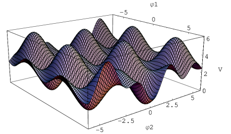
The periodicity of the potential implies an infinitely degenerate ground state and then the theory supports topologically charged excitations. A typical potential is plotted in Fig. 1. The vacuum configuration is related to the fundamental weights (see sections 3, 4 and the Appendix). For the moment, consider the fields $\Phi_{1}$ and $\Phi_{2}$ and the vacuum lattice defined by

$$(\Phi_{1}\,,\,\Phi_{2})=\frac{2\pi}{\beta_{0}}(\frac{n_{1}}{\nu_{1}}\,,\,\frac{n_{2}}{\nu_{2}}),\,\,\,\,\,n_{a}\in\leavevmode\hbox{\sf Z\kern-3.99994ptZ}.$$ (9)

Figure 1: GSG potential $V$ for the parameter values $\nu_{1}=1/2,\,\,\delta_{1}=2,\,\,\delta_{2}=1,\,\,\nu_{2}=1,\,\,r=s=1,\,\,\beta_{0}=1,\,\,\mu_{1}=\mu_{2}=1$.

It is convenient to write the equations of motion in terms of the independent fields $\varphi_{1}$ and $\varphi_{2}$

$$\partial^{2}\varphi_{1} = -\mu_{1}\beta_{1}\Delta_{11}\mbox{sin}[\beta_{1}(2\varphi_{1}-\varphi_{2})]-\mu_{2}\beta_{2}\Delta_{12}\mbox{sin}[\beta_{2}(2\varphi_{2}-\varphi_{1})]+$$ (10)

$$\mu_{3}\beta_{3}\Delta_{13}\mbox{sin}[\beta_{3}(r\varphi_{1}+s\varphi_{2})]$$

$$\partial^{2}\varphi_{2} = -\mu_{1}\beta_{1}\Delta_{21}\mbox{sin}[\beta_{1}(2\varphi_{1}-\varphi_{2})]-\mu_{2}\beta_{2}\Delta_{22}\mbox{sin}[\beta_{2}(2\varphi_{2}-\varphi_{1})]+$$ (11)

$$\mu_{3}\beta_{3}\Delta_{23}\mbox{sin}[\beta_{3}(r\varphi_{1}+s\varphi_{2})],$$

where

$$A = \beta_{0}^{2}\nu_{1}^{2}(4+\delta^{2}+\delta_{1}^{2}\rho_{1}^{2}r^{2}),\,\,\,\,B=\beta_{0}^{2}\nu_{1}^{2}(1+4\delta^{2}+\delta_{1}^{2}\rho_{1}^{2}s^{2}),$$

$$C = \beta_{0}^{2}\nu_{1}^{2}(2+2\delta^{2}+\delta_{1}^{2}\rho_{1}^{2}r\,s),$$

$$\Delta_{11} = (C-2B)/\Delta,\,\,\,\,\Delta_{12}=(B-2C)/\Delta,\,\,\,\,\Delta_{13}=(r\,B+s\,C)/\Delta,$$

$$\Delta_{21} = (A-2C)/\Delta,\,\,\,\,\Delta_{22}=(C-2A)/\Delta,\,\,\,\,\Delta_{23}=(r\,C+s\,A)/\Delta$$

$$\Delta = C^{2}-AB,\,\,\,\,\delta=\frac{\delta_{1}}{\delta_{2}}\rho_{0},\,\,\,\,\rho_{1}=\frac{3}{2r+s}$$

Notice that the eqs. of motion (10)-(11) exhibit the symmetry

$$\varphi_{1}\leftrightarrow\varphi_{2},\,\,\,\,\mu_{1}\leftrightarrow\mu_{2},\,\,\,\nu_{1}\leftrightarrow\nu_{2},\,\,\,\delta_{1}\leftrightarrow\delta_{2},\,\,\,r\leftrightarrow s$$ (12)

Some type of coupled sine-Gordon models have been considered in connection to various interesting physical problems [32]. For example a system of two coupled SG models has been proposed in order to describe the dynamics of soliton excitations in deoxyribonucleic acid (DNA) double helices [33]. In general these type of equations have been solved by perturbation methods around decoupled sine-Gordon exact solitons.

The system of equations (10)-(11) for certain choice of the parameters $r$ and $s$ will be derived in section 3 in the context of the $sl(3)$ ATM type models, in which the fields $\varphi_{1}$ and $\varphi_{2}$ couple to some Dirac spinors in such a way that the model exhibits a local gauge invariance. The ATM relevant equations of motion have been solved using a hybrid of the Hirota and Dressing methods [34]. However, in this reference the physical spectrum of solitons and kinks of the theory, related to a convenient gauge fixing of the model, have not been discussed, even though the topological and Noether currents equivalence has been verified. The appearance of the so-called tau functions, in order to find soliton solutions in integrable models, is quite a general result in the both Dressing and Hirota approaches. In this section, we will find soliton and kink type solutions of the GSG model (10)-(11) and closely follow the spirit of the above hybrid method approach to find soliton solutions.

The general tau function for an $n-$soliton solution of the gauge unfixed ATM model has the form [34, 35]

$$\tau = \sum_{p_{1}.....p_{n}=0}^{2}c_{p_{1}.....p_{n}}\mbox{exp}[p_{1}\Gamma_{i_{1}}(z_{1})+...+p_{n}\Gamma_{i_{n}}(z_{n})],$$

$$z_{i}=\gamma_{i}(x-v_{i}\,t),\,\,\,\,\,c_{p_{1}.....p_{n}}\in\leavevmode\hbox{\,$\vrule height=6.45831pt,width=0.4pt,depth=0.0pt\kern-3.00003pt{\rm C}$}$$

Since the GSG model describes the strong coupling sector (soliton spectrum) of the ATM model [14, 15] then one can guess the following Ansatz for the tau functions of the GSG model

$$e^{-i\beta_{0}\frac{\varphi_{1}}{2}}=\frac{\tau_{1}}{\tau_{0}},\,\,\,\,\,e^{-i\beta_{0}\frac{\varphi_{2}}{2}}=\frac{\tau_{2}}{\tau_{0}},$$ (14)

where the tau functions $\tau_{i}\,(i=0,1,2)$ are assumed to be of the form (2). We will see that the Ansatz (14) provides soliton and kink type solutions of the model (10)-(11), in this way justifying a posteriori the assumption made for the relevant tau functions.

Assuming that the fields $\varphi_{a}\,(a=1,2)$ are real, from (14) one can write

$$\varphi_{1,\,2} = \frac{4}{\beta_{0}}\mbox{arctan}[F(\tau_{1,\,2},\tau_{0})]$$ (15)

$$F \equiv \frac{e_{1}\Big{(}[Re(\tau_{1,\,2})]^{2}+[Im(\tau_{1,\,2})]^{2}\Big{)}-\Big{(}Re(\tau_{1,\,2})Re(\tau_{0})+Im(\tau_{1,\,2})Im(\tau_{0})\Big{)}}{\Big{[}Im(\tau_{1,\,2})*Re(\tau_{0})-Re(\tau_{1,\,2})*Im(\tau_{0})\Big{]}},$$

$$e_{1} = \pm 1$$ (16)

In terms of the tau functions the system of equations (10)-(11) becomes

$$\frac{2i}{\beta^{2}_{0}}\Big{[}\frac{\partial^{2}\tau_{1}}{\tau_{1}}-\frac{(\partial\tau_{1})^{2}}{\tau_{1}^{2}}-\frac{\partial^{2}\tau_{0}}{\tau_{0}}+\frac{(\partial\tau_{0})^{2}}{\tau_{0}^{2}}\Big{]}+\frac{\beta_{1}\mu_{1}\Delta_{11}}{2i}\Big{[}\frac{(\tau_{2}\tau_{0})^{4\nu_{1}}-\tau_{1}^{8\nu_{1}}}{(\tau_{2}\tau_{0})^{2\nu_{1}}\tau_{1}^{4\nu_{1}}}\Big{]} +$$

$$\frac{\beta_{2}\mu_{2}\Delta_{12}}{2i}\Big{[}\frac{(\tau_{1}\tau_{0})^{4\nu_{2}}-\tau_{2}^{8\nu_{2}}}{(\tau_{1}\tau_{0})^{2\nu_{2}}\tau_{2}^{4\nu_{2}}}\Big{]}-\frac{\beta_{3}\mu_{3}\Delta_{13}}{2i}\Big{[}\frac{(\tau_{0})^{4\nu_{3}(r+s)}-\tau_{1}^{4r\nu_{3}}\tau_{2}^{4s\nu_{3}}}{(\tau_{2})^{2s\nu_{3}}(\tau_{1})^{2r\nu_{3}}\tau_{0}^{2\nu_{3}(r+s)}}\Big{]} = 0,$$ (17)

$$\frac{2i}{\beta^{2}_{0}}\Big{[}\frac{\partial^{2}\tau_{2}}{\tau_{2}}-\frac{(\partial\tau_{2})^{2}}{\tau_{2}^{2}}-\frac{\partial^{2}\tau_{0}}{\tau_{0}}+\frac{(\partial\tau_{0})^{2}}{\tau_{0}^{2}}\Big{]}+\frac{\beta_{1}\mu_{1}\Delta_{21}}{2i}\Big{[}\frac{(\tau_{2}\tau_{0})^{4\nu_{1}}-\tau_{1}^{8\nu_{1}}}{(\tau_{2}\tau_{0})^{2\nu_{1}}\tau_{1}^{4\nu_{1}}}\Big{]} +$$

$$\frac{\beta_{2}\mu_{2}\Delta_{22}}{2i}\Big{[}\frac{(\tau_{1}\tau_{0})^{4\nu_{2}}-\tau_{2}^{8\nu_{2}}}{(\tau_{1}\tau_{0})^{2\nu_{2}}\tau_{2}^{4\nu_{2}}}\Big{]}-\frac{\beta_{3}\mu_{3}\Delta_{23}}{2i}\Big{[}\frac{(\tau_{0})^{4\nu_{3}(r+s)}-\tau_{1}^{4r\nu_{3}}\tau_{2}^{4s\nu_{3}}}{(\tau_{2})^{2s\nu_{3}}(\tau_{1})^{2r\nu_{3}}\tau_{0}^{2\nu_{3}(r+s)}}\Big{]} = 0.$$ (18)

We will see that the 1-soliton and 1-kink type solutions are related to half-integer or integer values of the parameters $\nu_{i}$ and the values $r,s\,=\,0,1$. In the next subsections we write the 1-antisoliton, 1-antikink and bounce type solutions, and in order to perform the cumbersome computations we resort to the MAPLE program.

2.1 One soliton associated to $\varphi_{1}$

Consider the tau functions

$$\tau_{0}=1+i\,d\,\mbox{exp}[\gamma(x-vt)];\,\,\,\,\tau_{1}=1-i\,d\,\mbox{exp}[\gamma(x-vt)];\,\,\,\,\tau_{2}=1+i\,d\,\mbox{exp}[\gamma(x-vt)].$$

This choice satisfies the system of equations (17)-(18) for the set of parameters

$$\nu_{1}=1/2,\,\,\delta_{1}=2,\,\,\delta_{2}=1,\,\,\nu_{2}=1,\,\,\nu_{3}=1,\,\,r=1.$$ (19)

provided that

$$13\mu_{3}=5\mu_{2}-4\mu_{1},\,\,\,\,\gamma^{2}_{1}=\frac{1}{13}(6\mu_{2}+3\mu_{1}).$$ (20)

Now, taking $e_{1}=1$ in Eq. (16) and the relation (15) one has

$$\varphi_{1}=-\frac{4}{\beta_{0}}\mbox{arctan}\{d\,\,\mbox{exp}[\gamma_{1}(x-vt)]\},\,\,\,\,\varphi_{2}=0.$$ (21)

This solution is precisely the sine-Gordon 1-antisoliton associated to the field $\varphi_{1}$ with mass $M_{1}=\frac{8\gamma_{1}}{\beta^{2}_{0}}$. We plot a soliton of this type in Fig. 3.

2.2 One soliton associated to $\varphi_{2}$

Next, let us consider the tau functions

$$\tau_{0}=1+i\,d\,\mbox{exp}[\gamma(x-vt)],\,\,\,\,\tau_{1}=1+i\,d\,\mbox{exp}[\gamma(x-vt)],\,\,\,\,\tau_{2}=1-i\,d\,\mbox{exp}[\gamma(x-vt)]$$

This set of tau functions solves the system (17)-(18) for the choice of parameters

$$\nu_{1}=1,\,\,\delta_{1}=1,\,\,\delta_{2}=2,\,\,\nu_{2}=1/2,\,\,\nu_{3}=1,\,\,s=1$$ (22)

provided that

$$13\mu_{3}=5\mu_{1}-4\mu_{2},\,\,\,\,\gamma^{2}_{2}=\frac{1}{13}(6\mu_{1}+3\mu_{2})$$ (23)

Now, choose $e_{1}=1$ in (16) and through (15) one can get

$$\varphi_{2}=-\frac{4}{\beta_{0}}\mbox{arctan}\{d\,\mbox{exp}[\gamma_{2}(x-vt)]\},\,\,\,\,\varphi_{1}=0$$ (24)

Similarly, this is the sine-Gordon 1-antisoliton associated to the field $\varphi_{2}$ with mass $M_{2}=\frac{8\gamma_{2}}{\beta^{2}_{0}}$ and its profile is of the type shown in Fig 3.

2.3 Two one-solitons associated to $\varphi\equiv\varphi_{1,\,2}$

Now, let us consider the tau functions

$$\tau_{0}=1+i\,d\,\,\mbox{exp}[\gamma(x-vt)],\,\,\,\,\tau_{1}=1-i\,d\,\,\mbox{exp}[\gamma(x-vt)],\,\,\,\,\tau_{2}=1-i\,d\,\,\mbox{exp}[\gamma(x-vt)].$$

This choice satisfies (17)-(18) for

$$\nu_{1}=1,\,\,\delta_{1}=1/2,\,\,\nu_{2}=1,\,\,\delta_{2}=1/2,\,\,\nu_{3}=1/2,\,\,r=s=1,$$ (25)

provided that

$$d^{2}=1,\,\,\,\,38\gamma^{2}_{3}=25\mu_{1}+13\mu_{2}+19\mu_{3}$$ (26)

Now, taking $e_{1}=1$ in (15) one has

$$\varphi_{1} = \varphi_{2}\equiv\hat{\varphi}_{1},\,\,\,\,$$ (27)

$$\hat{\varphi}_{1} = -\frac{4}{\beta_{0}}\mbox{arctan}\{d\,\,\,\mbox{exp}[\gamma_{3}(x-vt)]\}.$$ (28)

This is a sine-Gordon 1-antisoliton associated to both fields $\varphi_{1,\,2}$ in the particular case when they are equal to each other. It possesses a mass $M_{3}=\frac{8\gamma_{3}}{\beta_{0}^{2}}$.

In view of the symmetry (12) we are able to write

$$d^{2}=1,\,\,\,\,38\gamma^{2}_{4}=25\mu_{2}+13\mu_{1}+19\mu_{3},$$ (29)

and then on has another soliton of this type

$$\varphi_{1} = \varphi_{2}\equiv\hat{\varphi}_{2},\,$$ (30)

$$\hat{\varphi}_{2} = -\frac{4}{\beta_{0}}\mbox{arctan}\{d\,\,\,\mbox{exp}[\gamma_{4}(x-vt)]\}.$$ (31)

It possesses a mass $M_{4}=\frac{8\gamma_{4}}{\beta_{0}^{2}}$. This 1-antisoliton is of the type shown in Fig. 3.

The GSG system (10)-(11) reduces to the usual SG equation for each choice of the parameters (19), (22) and (25), respectively. Then, the $n-$soliton solutions in each case can be constructed as in the ordinary sine-Gordon model by taking appropriate tau functions in (2)-(14).

The baryon number associated to each of the above 1-soliton solutions has been computed in connection to QCD₂, and it takes the same value $B=N_{c}$ (in this normalization the quark has baryon number $B_{quark}=1$) [6].

A modified model with rich soliton dynamics is the so-called stepwise sine-Gordon model in which the system parameter depends on the sign of the SG field [36]. It would be interesting to consider the above GSG model along the lines of this reference.

2.4 Mass splitting of solitons

It is interesting to write some relations among the various soliton masses

$$M_{3}^{2}=\frac{1}{76}(109M_{2}^{2}+5M_{1}^{2});\,\,\,\,M_{4}^{2}=\frac{1}{76}(109M_{1}^{2}+5M_{2}^{2});$$ (32)

If $\mu_{1}=\mu_{2}$ then we have the degeneracy $M_{1}=M_{2}$, and $M_{3}=M_{4}=\sqrt{3/2}M_{1}$. Notice that if $M_{1}\neq M_{2}$ then $M_{3}<M_{1}+M_{2}$ and $M_{4}<M_{1}+M_{2}$, and the third and fourth solitons are stable in the sense that energy is required to dissociate them.

2.5 Kinks of the reduced two-frequency sine-Gordon model

In the system (10)-(11) we perform the following reduction $\varphi\equiv\varphi_{1}=\varphi_{2}$ such that

$$\Phi_{1}=\Phi_{2},\,\,\,\Phi_{3}=q\,\Phi_{1},$$ (33)

with $q$ being a real number. Therefore, using the constraint (4) one can deduce the relationships

$$\delta_{1}=\frac{q}{2},\,\,\,\delta=1.$$ (34)

Moreover, for consistency of the system of equations (10)-(11) we have to impose the relationships

$$\nu_{1}\mu_{1}\Delta_{11}+\nu_{2}\mu_{2}\Delta_{12} = \nu_{1}\mu_{1}\Delta_{21}+\nu_{2}\mu_{2}\Delta_{22},$$ (35)

$$\Delta_{13} = \Delta_{23}.$$ (36)

These relations imply

$$\delta^{2}=1,\,\,\,\mu_{1}=\delta\,\,\mu_{2}$$ (37)

.

Taking into account the relations (34) and (37) together with (5) we get

$$\mu_{1}=\mu_{2},\,\,\,\,\delta=1,\,\,\,\nu_{1}=\nu_{2},\,\,\,\nu_{3}=\frac{q}{2}\nu_{1},\,\,r=s=1.$$ (38)

Thus the system of Eqs.(10)-(11) reduce to

$$\partial^{2}\Phi = -\frac{\mu_{1}}{\nu_{1}}\,\mbox{sin}(\nu_{1}\Phi)-\frac{\mu_{3}\delta_{1}}{\nu_{1}}\mbox{sin}(q\,\nu_{1}\Phi),\,\,\,\,\,\Phi\equiv\beta_{0}\varphi.$$ (39)

This is the so-called two-frequency sine-Gordon model (DSG) and it has been the subject of much interest in the last decades, from the mathematical and physical points of view. It encounters many interesting physical applications, see e.g. [11, 12, 31, 32].

If the parameter $q$ satisfies

$$q=\frac{n}{m}\,\in\,\leavevmode\hbox{\,$\vrule height=6.45831pt,width=0.4pt,depth=0.0pt\kern-3.00003pt{\rm Q}$}$$ (40)

with $m,\,n$ being two relative prime positive integers, then the potential $\frac{\mu_{1}}{\nu_{1}^{2}}(1-\mbox{cos}(\nu_{1}\Phi))+\frac{\mu_{3}}{2\nu_{1}^{2}}(1-\mbox{cos}(q\nu_{1}\Phi))$ associated to the model (39) is periodic with period

$$\frac{2\pi}{\nu_{1}}m=\frac{2\pi}{q\,\nu_{1}}n.$$ (41)

As mentioned above the theory (39) possesses topological excitations. The fundamental topological excitations degenerates in the $\mu_{1}=0$ limit to an $n-$soliton state of the relevant sine-Gordon model and similarly in the limit $\mu_{3}=0$ it will be an $m$-soliton state. For general values of the parameters $\mu_{1},\,\mu_{3},\,\delta_{1},\,\nu_{1}$ the solitons are in some sense “confined” inside the topological excitations which become in this form some composite objects. On the other hand, if $q\notin\leavevmode\hbox{\,$\vrule height=6.45831pt,width=0.4pt,depth=0.0pt\kern-3.00003pt{\rm Q}$}$ then the potential is not periodic, so, there are no topologically charged excitations and the solitons are completely confined [9, 10].

The model (39) in the limit $\mu_{1}=0$ reduces to

$$\partial^{2}\varphi=-\frac{\mu_{3}q}{2\nu_{1}\beta_{0}}\,\mbox{sin}(q\nu_{1}\beta_{0}\varphi).$$ (42)

For later discussion we record here the mass of the soliton associated to this equation,

$$M_{\mu_{3}}=\frac{8}{(q\nu_{1}\beta_{0})^{2}}\sqrt{q^{2}\mu_{3}/2}.$$ (43)

Correspondingly in the limit $\mu_{3}=0$ one has

$$\partial^{2}\varphi=-\frac{mu_{1}}{\nu_{1}\beta_{0}}\,\mbox{sin}(\nu_{1}\beta_{0}\varphi)$$ (44)

with associated soliton mass

$$M_{\mu_{1}}=\frac{8}{(\nu_{1}\beta_{0})^{2}}\sqrt{\mu_{1}}$$ (45)

Notice that other possibilities to perform the reduction of type (33) encounter some inconsistencies, e.g. the attempt to implement the reduction $\Phi_{1}=\Phi_{3},\,\,\Phi_{2}=q^{\prime}\,\Phi_{1}$ implies $\delta_{1,\,2}^{2}<0$ which is a contradiction since $\delta_{1,\,2}$ are real numbers by definition. The same inconsistency occurs when one tries to reduce the $sl(3)$ GSG model to a three-frequency SG model. We expect that the three and higher frequency models [37] will be related to $sl(N),\,N\geq 4,$ GSG models.

In the following we will provide some kink solutions for particular set of parameters. Consider

$$\nu_{1}=1/2,\,\,\delta_{1}=\delta_{2}=1,\,\,\nu_{2}=1/2,\,\,\,\nu_{3}=1/2\,\,\,\mbox{and}\,\,\,q=2,\,n=2,\,m=1$$ (46)

which satisfy (38) and (40), respectively. This set of parameters provide the so-called double sine-Gordon model (DSG). Its potential $-[4\mu_{1}(\mbox{cos}\frac{\Phi}{2}-1)+2\mu_{3}(\mbox{cos}\Phi-1)]$ has period $4\pi$ and has extrema at $\Phi=2\pi p_{1}$, and  $\Phi=4\pi p_{2}\pm 2\mbox{cos}^{-1}[1-|\mu_{1}/(2\mu_{3})|]$ with $p_{1},p_{2}\in\leavevmode\hbox{\sf Z\kern-3.99994ptZ}$; the second extrema exists only if $|\mu_{1}/(2\mu_{3})|<1$. From the mathematical point of view the DSG model belongs to a class of theories with partial integrability [38]. Depending on the values of the parameters $\beta_{0},\,\mu_{1},\,\mu_{3}$ the quantum field theory version of the DSG model presents a variety of physical effects, such as the decay of the false vacuum, a phase transition, confinement of the kinks and the resonance phenomenon due to unstable bound states of excited kink-antikink states (see [12] and references therein). The semi-classical spectrum of neutral particles in the DSG theory is investigated in [39]. Let us mention that the DSG model has recently been in the center of some controversy regarding the computation of its semiclassical spectrum, see [12, 13].

Interestingly the functions

$$\tau_{0} = 1+i\,d\,\mbox{exp}[\gamma(x-vt)]+h\,\mbox{exp}[2\gamma(x-vt)],\,\,\,$$

$$\tau_{1} = 1-i\,d\,\mbox{exp}[\gamma(x-vt)]+h\,\mbox{exp}[2\gamma(x-vt)],$$ (47)

satisfy the equation (39) for the parameters (46) provided

$$e^{-i\Phi/2} = \tau_{1}/\tau_{0}$$ (48)

$$\gamma^{2} = \mu_{1}+2\mu_{3},\,\,\,h=-\frac{\mu_{1}}{4},\,\,\,\,e_{1}=-1$$ (49)

The general solution of this type can be written as

$$\Phi:=4\,\mbox{arctan}\left[\frac{1}{d}\,\,\frac{1+h\,\,\mbox{exp}[2\gamma(x-vt)]}{\mbox{exp}[\gamma(x-vt)]}\right]$$ (50)

2.5.1 DSG kink ($h<0,\,\mu_{i}>0$)

For the choice of parameters $h<0,\,\mu_{i}>0$ in (49) the equation (50) provides

$$\varphi:=\frac{4}{\beta_{0}}\mbox{arctan}\left[\frac{-2|h|^{1/2}}{d}\,\,\mbox{sinh}[\gamma_{K}\,(x-vt)+a_{0}]\right],\,\,\,\,\gamma_{K}\equiv\pm\sqrt{\mu_{1}+2\mu_{3}},$$ (51)

$$a_{0}=\frac{1}{2}\mbox{ln}|h|.$$

This is the DSG 1-kink solution with mass

$$M_{K}=\frac{16}{\beta_{0}^{2}}\gamma_{K}\left[1+\frac{\mu_{1}}{\sqrt{2\mu_{3}(\mu_{1}+2\mu_{3})}}\mbox{ln}(\frac{\sqrt{\mu_{1}+2\mu_{3}}+\sqrt{2\mu_{3}}}{\sqrt{\mu_{1}}})\right].$$ (52)

Notice that in the limit $\mu_{1}\rightarrow 0$ the kink mass becomes $M_{K}=\frac{16}{\beta_{0}^{2}}\sqrt{2\mu_{3}}$, which is twice the soliton mass (43) of the model (42) for the parameters $\nu_{1}=1/2,\,q=2$. Similarly, in the limit $\mu_{3}\rightarrow 0$ the kink mass becomes $\frac{8}{(\beta_{0}/2)^{2}}\sqrt{\mu_{1}}$, which is the soliton mass (45) of the model (44) for $\nu_{1}=1/2,\,q=2$; thus in this case the coupling constant is $\beta_{0}/2$. As discussed above these solitons get in some sense “confined” inside the kink if the parameters satisfy $\mu_{i}\neq 0$. The 1-antikink is plotted in Fig. 4. Moreover, the relevant baryon number associated to this DSG kink becomes $B_{kink}=4N_{c}$ [6].

2.5.2 Bounce-like solution ($h>0$,  $\mu_{1}<0$)

For the parameters $h>0$,  $\mu_{1}<0$ one gets from (50)

$$\varphi:=\frac{4}{\beta_{0}}\mbox{arctan}\left[\frac{2h^{1/2}}{d}\,\,\mbox{cosh}[\gamma^{\prime}(x-vt)+a_{0}^{\prime}]\right],\,\,\,\,\,\gamma^{\prime}=2\mu_{3}-|\mu_{1}|,\,\,\,\,a_{0}^{\prime}=\frac{1}{2}\mbox{ln}h$$ (53)

This is the bounce-like solution and interpolates between the two vacuum values $2\pi$ and $4\pi-2\mbox{arcos}(1-|\mu_{1}/2\mu_{3}|)$ and then it comes back. Since $2\pi$ is a false vacuum position this solution is not related to any stable particle in the quantum theory [12]. In Fig. 2 we plot this profile.

Figure 2: Bounce-like solution ($\frac{\beta_{0}}{4}\varphi$) plotted for $\mu_{2}=-0.0000001,\,\mu_{3}=0.001,\,d=-2$.

3 Classical GSG as a reduced Toda model coupled to matter

In this section we provide the algebraic construction of the $sl(3)$ affine Toda model coupled to matter fields (ATM) and closely follows refs. [15, 34, 41] but the reduction process to arrive at the classical GSG model is new. The previous treatments of the $sl(3)$ ATM model used the symplectic and on-shell decoupling methods to unravel the classical GSG and generalized massive Thirring (GMT) dual theories describing the strong/weak coupling sectors of the ATM model [14, 15, 42]. The ATM model describes some scalars coupled to spinor (Dirac) fields in which the system of equations of motion has a local gauge symmetry. In this way one includes the spinor sector in the discussion and conveniently gauge fixing the local symmetry by setting some spinor bilinears to constants we are able to decouple the scalar (Toda) fields from the spinors, the final result is a direct construction of the classical generalized sine-Gordon model (cGSG) involving only the scalar fields. In the spinor sector we are left with a system of equations in which the Dirac fields couple to the cGSG fields.

The zero curvature condition (131) gives the following equations of motion [41]

$$\frac{\partial^{2}\theta_{a}}{4i\,e^{\eta}} = m^{1}_{\psi}[e^{\eta-i\phi_{a}}\widetilde{\psi}_{R}^{l}\psi_{L}^{l}+e^{i\phi_{a}}\widetilde{\psi}_{L}^{l}\psi_{R}^{l}]+m^{3}_{\psi}[e^{-i\phi_{3}}\widetilde{\psi}_{R}^{3}\psi_{L}^{3}+e^{\eta+i\phi_{3}}\widetilde{\psi}_{L}^{3}\psi_{R}^{3}];$$

$$\,\,\,\,a=1,2$$ (54)

$$-\frac{\partial^{2}\widetilde{\nu}}{4} = im^{1}_{\psi}e^{2\eta-\phi_{1}}\widetilde{\psi}_{R}^{1}\psi_{L}^{1}+im^{2}_{\psi}e^{2\eta-\phi_{2}}\widetilde{\psi}_{R}^{2}\psi_{L}^{2}+im^{3}_{\psi}e^{\eta-\phi_{3}}\widetilde{\psi}_{R}^{3}\psi_{L}^{3}+{\bf m}^{2}e^{3\eta},\,\,$$ (55)

$$-2\partial_{+}\psi_{L}^{1} = m^{1}_{\psi}e^{\eta+i\phi_{1}}\psi_{R}^{1},\,\,\,\,\,\,\,\,\,\,\,\,\,\,\,-2\partial_{+}\psi_{L}^{2}\,=\,m^{2}_{\psi}e^{\eta+i\phi_{2}}\psi_{R}^{2},$$ (56)

$$2\partial_{-}\psi_{R}^{1} = m^{1}_{\psi}e^{2\eta-i\phi_{1}}\psi_{L}^{1}+2i\Big{(}\frac{m^{2}_{\psi}m^{3}_{\psi}}{im^{1}_{\psi}}\Big{)}^{1/2}e^{\eta}(-\psi_{R}^{3}\widetilde{\psi}_{L}^{2}e^{i\phi_{2}}-\widetilde{\psi}_{R}^{2}\psi_{L}^{3}e^{-i\phi_{3}}),$$ (57)

$$2\partial_{-}\psi_{R}^{2} = m^{2}_{\psi}e^{2\eta-i\phi_{2}}\psi_{L}^{2}+2i\Big{(}\frac{m^{1}_{\psi}m^{3}_{\psi}}{im^{2}_{\psi}}\Big{)}^{1/2}e^{\eta}(\psi_{R}^{3}\widetilde{\psi}_{L}^{1}e^{i\phi_{1}}+\widetilde{\psi}_{R}^{1}\psi_{L}^{3}e^{-i\phi_{3}}),$$ (58)

$$-2\partial_{+}\psi_{L}^{3} = m^{3}_{\psi}e^{2\eta+i\phi_{3}}\psi_{R}^{3}+2i\Big{(}\frac{m^{1}_{\psi}m^{2}_{\psi}}{im^{3}_{\psi}}\Big{)}^{1/2}e^{\eta}(-\psi_{L}^{1}\psi_{R}^{2}e^{i\phi_{2}}+\psi_{L}^{2}\psi_{R}^{1}e^{i\phi_{1}}),$$ (59)

$$2\partial_{-}\psi_{R}^{3} = m^{3}_{\psi}e^{\eta-i\phi_{3}}\psi_{L}^{3},\,\,\,\,\,\,\,\,\,\,\,\,2\partial_{-}\widetilde{\psi}_{R}^{1}\,=\,m^{1}_{\psi}e^{\eta+i\phi_{1}}\widetilde{\psi}_{L}^{1},$$ (60)

$$-2\partial_{+}\widetilde{\psi}_{L}^{1} = m^{1}_{\psi}e^{2\eta-i\phi_{1}}\widetilde{\psi}_{R}^{1}+2i\Big{(}\frac{m^{2}_{\psi}m^{3}_{\psi}}{im^{1}_{\psi}}\Big{)}^{1/2}e^{\eta}(-\psi_{L}^{2}\widetilde{\psi}_{R}^{3}e^{-i\phi_{3}}-\widetilde{\psi}_{L}^{3}\psi_{R}^{2}e^{i\phi_{2}}),$$ (61)

$$-2\partial_{+}\widetilde{\psi}_{L}^{2} = m^{2}_{\psi}e^{2\eta-i\phi_{2}}\widetilde{\psi}_{R}^{2}+2i\Big{(}\frac{m^{1}_{\psi}m^{3}_{\psi}}{im^{2}_{\psi}}\Big{)}^{1/2}e^{\eta}(\psi_{L}^{1}\widetilde{\psi}_{R}^{3}e^{-i\phi_{3}}+\widetilde{\psi}_{L}^{3}\psi_{R}^{1}e^{i\phi_{1}}),$$ (62)

$$2\partial_{-}\widetilde{\psi}_{R}^{2} = m^{2}_{\psi}e^{\eta+i\phi_{2}}\widetilde{\psi}_{L}^{2},\,\,\,\,\,\,\,\,\,\,\,\,\,\,\,\,-2\partial_{+}\widetilde{\psi}_{L}^{3}\,=\,m^{3}_{\psi}e^{\eta-i\phi_{3}}\widetilde{\psi}_{R}^{3},$$ (63)

$$2\partial_{-}\widetilde{\psi}_{R}^{3} = m^{3}_{\psi}e^{2\eta+i\phi_{3}}\widetilde{\psi}_{L}^{3}+2i\Big{(}\frac{m^{1}_{\psi}m^{2}_{\psi}}{im^{3}_{\psi}}\Big{)}^{1/2}e^{\eta}(\widetilde{\psi}_{R}^{1}\widetilde{\psi}_{L}^{2}e^{i\phi_{2}}-\widetilde{\psi}_{R}^{2}\widetilde{\psi}_{L}^{1}e^{i\phi_{1}}),$$ (64)

$$\partial^{2}\eta = 0,$$ (65)

where $\phi_{1}\equiv 2\theta_{1}-\theta_{2},\,\phi_{2}\equiv 2\theta_{2}-\theta_{1},\,\phi_{3}\equiv\theta_{1}+\theta_{2}$. Therefore, one has

$$\phi_{3}=\phi_{1}+\phi_{2}$$ (66)

The $\theta$ fields are considered to be in general complex fields. In order to define the classical generalized sine-Gordon model we will consider these fields to be real.

Apart from the conformal invariance the above equations exhibit the $\Big{(}U(1)_{L}\Big{)}^{2}\otimes\Big{(}U(1)_{R}\Big{)}^{2}$ left-right local gauge symmetry

$$\theta_{a} \rightarrow \theta_{a}+\xi_{+}^{a}(x_{+})+\xi_{-}^{a}(x_{-}),\,\,\,\,a=1,2$$ (67)

$$\widetilde{\nu} \rightarrow \widetilde{\nu}\;;\qquad\eta\rightarrow\eta$$ (68)

$$\psi^{i} \rightarrow e^{i(1+\gamma_{5})\Xi_{+}^{i}(x_{+})+i(1-\gamma_{5})\Xi_{-}^{i}(x_{-})}\,\psi^{i},$$ (69)

$$\,\,\,\,\widetilde{\psi}^{i} \rightarrow e^{-i(1+\gamma_{5})(\Xi_{+}^{i})(x_{+})-i(1-\gamma_{5})(\Xi_{-}^{i})(x_{-})}\,\widetilde{\psi}^{i},\,\,\,i=1,2,3;$$

$$\Xi^{1}_{\pm}\equiv\pm\xi_{\pm}^{2}\mp 2\xi_{\pm}^{1},\,\,\Xi^{2}_{\pm}\equiv\pm\xi_{\pm}^{1}\mp 2\xi_{\pm}^{2},\,\,\Xi_{\pm}^{3}\equiv\Xi_{\pm}^{1}+\Xi_{\pm}^{2}.$$

One can get global symmetries for $\xi_{\pm}^{a}=\mp\xi_{\mp}^{a}=$ constants. For a model defined by a Lagrangian these would imply the presence of two vector and two chiral conserved currents. However, it was found only half of such currents [34]. This is a consequence of the lack of a Lagrangian description for the $sl(3)^{(1)}$ CATM in terms of the $B$ and $F^{\pm}$ fields (see Appendix). So, the vector current

$$J^{\mu}=\sum_{j=1}^{3}m^{j}_{\psi}\bar{\psi}^{j}\gamma^{\mu}\psi^{j}$$ (71)

and the chiral current

$$J^{5\,\mu}=\sum_{j=1}^{3}m^{j}_{\psi}\bar{\psi}^{j}\gamma^{\mu}\gamma_{5}\psi^{j}+2\partial_{\mu}(m^{1}_{\psi}\theta_{1}+m^{2}_{\psi}\theta_{2})$$ (72)

are conserved

$$\partial_{\mu}J^{\mu}=0,\,\,\,\,\,\partial_{\mu}J^{5\,\mu}=0$$ (73)

The conformal symmetry is gauge fixed by setting

$$\eta=\mbox{const}.$$ (74)

The off-critical model obtained in this way exhibits the vector and topological currents equivalence [41, 42]

$$\sum_{j=1}^{3}m^{j}_{\psi}\bar{\psi}^{j}\gamma^{\mu}\psi^{j}\equiv\epsilon^{\mu\nu}\partial_{\nu}(m^{1}_{\psi}\theta_{1}+m^{2}_{\psi}\theta_{2}),\,\,\,\,\,\,\,m^{3}_{\psi}=m^{1}_{\psi}+m^{2}_{\psi},\,\,\,\,m^{i}_{\psi}>0.$$ (75)

Moreover, it has been shown that the soliton type solutions are in the orbit of the vacuum $\eta=0$.

In the next steps we implement the reduction process to get the cGSG model through a gauge fixing of the ATM theory. The local symmetries (67)-(3) can be gauge fixed through

$$i\bar{\psi}^{j}\psi^{j}=iA_{j}=\mbox{const.};\,\,\,\,\,\,\bar{\psi}^{j}\gamma_{5}\psi^{j}=0.$$ (76)

From the gauge fixing (76) one can write the following bilinears

$$\widetilde{\psi}_{R}^{j}\psi_{L}^{j}+\widetilde{\psi}_{L}^{j}\psi_{R}^{j}=0,\,\,\,\,\,j=1,2,3;$$ (77)

so, the eqs. (76) effectively comprises three gauge fixing conditions.

It can be directly verified that the gauge fixing (76) preserves the currents conservation laws (73), i.e. from the equations of motion (54)-(65) and the gauge fixing (76) together with (74) it is possible to obtain the currents conservation laws (73).

Taking into account the constraints (76) in the scalar sector, eqs. (54), we arrive at the following system of equations (set $\eta=0$)

$$\partial^{2}\theta_{1} = M^{1}_{\psi}\,\mbox{sin}\phi_{1}+M_{\psi}^{3}\,\mbox{sin}\phi_{3},$$ (78)

$$\,\,\,\partial^{2}\theta_{2} = M^{2}_{\psi}\,\mbox{sin}\phi_{2}+M^{3}_{\psi}\,\mbox{sin}\phi_{3},\,\,\,\,M^{i}_{\psi}\equiv 4A_{i}\,m_{\psi}^{i},\,\,\,\,i=1,2,3.$$ (79)

Define the fields $\varphi_{1},\,\varphi_{2}$ as

$$\varphi_{1} \equiv a\theta_{1}+b\theta_{2},\,\,\,\,\,\,\,\,a=\frac{4\nu_{2}-\nu_{1}}{3\beta_{0}\nu_{1}\nu_{2}},\,\,\,d=\frac{4\nu_{1}-\nu_{2}}{3\beta_{0}\nu_{1}\nu_{2}}$$ (80)

$$\varphi_{2} \equiv c\theta_{1}+d\theta_{2},\,\,\,\,\,\,\,\,b=-c=\frac{2(\nu_{1}-\nu_{2})}{3\beta_{0}\nu_{1}\nu_{2}},\,\,\,\,\nu_{1},\nu_{2}\in\leavevmode\hbox{\rm I\kern-1.79993ptR}$$ (81)

Then, the system of equations (78)-(79) written in terms of the fields $\varphi_{1,\,2}$ becomes

$$\partial^{2}\varphi_{1} = aM^{1}_{\psi}\,\mbox{sin}[\beta_{0}\nu_{1}(2\varphi_{1}-\varphi_{2})]+bM^{2}_{\psi}\,\mbox{sin}[\beta_{0}\nu_{2}(2\varphi_{2}-\varphi_{1})]+$$ (82)

$$(a+b)M^{3}_{\psi}\,\mbox{sin}\beta_{0}[(2\nu_{1}-\nu_{2})\varphi_{1}+(2\nu_{2}-\nu_{1})\varphi_{2})],$$

$$\partial^{2}\varphi_{2} = cM^{1}_{\psi}\,\mbox{sin}[\beta_{0}\nu_{1}(2\varphi_{1}-\varphi_{2})]+dM^{2}_{\psi}\,\mbox{sin}[\beta_{0}\nu_{2}(2\varphi_{2}-\varphi_{1})]+$$ (83)

$$(c+d)M^{3}_{\psi}\,\mbox{sin}\beta_{0}[(2\nu_{1}-\nu_{2})\varphi_{1}+(2\nu_{2}-\nu_{1})\varphi_{2})]$$

The system of equations above considered for real fields $\varphi_{1,\,2}$ as well as for real parameters $M_{\psi}^{i},a,b,c,d,\beta_{0}$ defines the classical generalized sine-Gordon model (cGSG). Notice that this classical version of the GSG model derived from the ATM theory is a submodel of the GSG model (10)-(11), defined in section 2, for the particular parameter values $r=\frac{2\nu_{1}-\nu_{2}}{\nu_{3}},\,s=\frac{2\nu_{2}-\nu_{1}}{\nu_{3}}$ and the convenient identifications of the parameters in the coefficients of the sine functions of the both models.

The following reduced models can be obtained from the system (82)-(83):

i)SG submodels
i.1) For $\nu_{2}=2\nu_{1}$  one has $M^{1}_{\psi}=M^{2}_{\psi}$ and the system
$\varphi_{2}=0$,   $\partial^{2}\varphi_{1}=M^{1}_{\psi}\frac{3\nu_{1}}{\beta_{0}}\,\mbox{sin}\,\beta_{0}2\nu_{1}\varphi_{1}$.
i.2) For $\nu_{1}=2\nu_{2}$  one has $M^{1}_{\psi}=M^{2}_{\psi}$ and the system
$\varphi_{1}=0$,   $\partial^{2}\varphi_{2}=M^{2}_{\psi}\frac{3\nu_{2}}{\beta_{0}}\,\mbox{sin}\,\beta_{0}2\nu_{2}\varphi_{2}$.
i.3) For $\nu_{2}=\nu_{1}\equiv\nu$  and $\varphi_{1}=\varphi_{2}\equiv\hat{\varphi}_{A},\,(A=1,2)$, one gets the sub-models

i.3a) $M^{1}_{\psi}=M^{2}_{\psi},\,M^{3}_{\psi}=0$,   $\partial^{2}\hat{\varphi}_{1}=aM^{1}_{\psi}\,\mbox{sin}\,\beta_{0}\nu\hat{\varphi}_{1},$

i.3b) $M^{1}_{\psi}=M^{2}_{\psi}=0$,   $\partial^{2}\hat{\varphi}_{2}=aM^{3}_{\psi}\,\mbox{sin}\,\beta_{0}\nu\hat{\varphi}_{2}.$

ii) DSG sub-model
For $\nu_{1}=\nu_{2}$  and   $M^{1}_{\psi}=M^{2}_{\psi}$ one gets the sub-model $\varphi_{1}=\varphi_{2}\equiv\varphi$,   $\partial^{2}\varphi=aM^{1}_{\psi}\,\mbox{sin}\,\beta_{0}\nu_{1}\varphi+aM^{3}_{\psi}\,\mbox{sin}\,2\beta_{0}\nu_{1}\varphi$.

The sub-models i.1)-i.2) each one contains the ordinary sine-Gordon model (SG) and they were considered in the subsections 2.1 and 2.2, respectively; the sub-model i.3) supports two SG models with different soliton masses which must correspond to the construction in subsection 2.3; and the ii) case defines the double sine-Gordon model (DSG) studied in subsection 2.5. Other meaningful reductions are possible arriving at either SG or DSG model. Notice that the reductions above are particular cases of the sub-models in subsections 2.1, 2.2, 2.3 and 2.5, respectively, for relevant parameter identifications.

The spinor sector in view of the gauge fixing (76) can be parameterized conveniently as

$$\left(\begin{array}[]{c}\psi_{R}^{j}\\ \psi_{L}^{j}\end{array}\right)=\left(\begin{array}[]{c}\sqrt{A_{j}/2}\,u_{j}\\ i\sqrt{A_{j}/2}\,\frac{1}{v_{j}}\end{array}\right);\,\,\,\,\left(\begin{array}[]{c}\widetilde{\psi}_{R}^{j}\\ \widetilde{\psi}_{L}^{j}\end{array}\right)=\left(\begin{array}[]{c}\sqrt{A_{j}/2}\,v_{j}\\ -i\sqrt{A_{j}/2}\,\frac{1}{u_{j}}\end{array}\right).$$ (92)

Therefore, in order to find the spinor field solutions one can solve the eqs. (56)-(64) for the fields $u_{j},v_{j}$ for each solution given for the cGSG fields $\varphi_{1,\,2}$ of the system (82)-(83).

3.1 Physical solitons and kinks of the ATM model

The main feature of the one ‘solitons’ constructed in [34] is that for each positive root of $sl(3)$ there corresponds one soliton species associated to the fields $\phi_{1},\,\phi_{2},\,\phi_{3}$, respectively. The relevant solutions for the spinor fields together with the 1-‘solitons’ satisfy the relationship (75). The class of $2$-‘soliton’ solutions of $sl(3)$ ATM obtained in [34] behave as follows:  i) they are given by 6 species associated to the pair $(\alpha_{i},\alpha_{j}),\,i\leq j;\,\,i,j=1,2,3$; where the $\alpha$’s are the positive roots of $sl(3)$ Lie algebra. Each species $(\alpha_{i},\alpha_{i})$ solves the $sl(2)$ ATM submodel. ii) they satisfy the $U(1)$ vector and topological currents equivalence (75). However, the possible kink type solutions associated in a non-local way to the spinor bilinears and the relevant gauge fixing of the local symmetry (67)-(3) have not been discussed in the literature. In order to consider the physical spectrum of solitons and study its properties, such as their masses and scattering time delays, it is mandatory to take into account these questions which are related to the counting of the true physical degrees of freedom of the theory. Therefore, one must consider the possible soliton type solutions associated to each spinor bilinear. The relation between this type of ‘solitons’, say $\hat{\phi}_{j}$, and their relevant fermion bilinears must be non-local as suggested by the equivalence equation (75). So, we may have soliton solutions of type

$$\hat{\phi}_{j}=\int^{x}\,dx^{\prime}\,\bar{\psi}^{j}\gamma^{0}\psi^{j},\,\,\,\,\,\,j=1,2,3$$ (93)

At this stage one is able to enumerate the physical 1-soliton (1-antisoliton) spectrum associated to the gauge fixed ATM model. In fact, we have three ’kinks’ and their corresponding ’anti-kinks’ associated to the fields $\phi_{i}$ (i=1,2,3), and three kink and antikink pairs of type $\hat{\phi}_{j},\,j=1,2,3$. Thus, we have six kink and their relevant antikink solutions, but in order to record the physical soliton and anti-soliton excitations one must take into account the four constraints (66) and (77). Therefore, we expect to find four pairs of soliton and anti-soliton physical excitations in the spectrum. This feature is nicely reproduced in the cGSG sector of the ATM model; in fact, in the last section we were able to write four usual sine-Gordon models as possible reductions of the cGSG model. Namely, one soliton associated to the fields $\varphi_{1},\,\varphi_{2}$, respectively (subsections 2.1 and 2.2) and 1-solitons associated to the field $\varphi_{1}=\varphi_{2}\equiv\varphi_{A},\,A=1,2$, respectively (subsection 2.3). In the 2-kink (2-antikink) sector a similar argument will provide us ten physical 2-solitons and their relevant 2-antisoliton excitations, i.e. six pairs of 2-kink and 2-antikink solutions of type $\phi$ and $\hat{\phi}$, respectively, which give twenty four excitations, and taking into account the constraints (66) and (77) we are left with ten pairs of 2-solitons and 2-antisolitons. In fact, these ten 2-solitons correspond to the pairs we can form with the four species of 1-solitons in all possible ways. The same argument holds for the corresponding ten 2-antisolitons.

In this way the system (82)-(83) gives rise to a richer (anti)soliton spectrum and dynamics than the $\theta_{a}$ field ’soliton’ type solutions of the gauge unfixed model (54)-(64) found in [34]. Regarding this issue let us notice that in the procedure followed in ref. [34] the local symmetry (67)-(3) and the relevant gauge fixing has not been considered explicitly, therefore their ’solitons’ do not correspond to the GSG solitons obtained above.

Notice that the tau functions in section 2 possess the function $\gamma(x-vt)$ in their exponents, whereas the corresponding ones in the ATM theory have two times this function [34, 43]. This fact is reflected in the GSG soliton solutions which are two times the relevant solutions of the ATM model. It has been observed already in the $sl(2)$ case that the $\theta$ ‘soliton’ of the gauge unfixed $sl(2)$ ATM model (see eq. (2.22) of [43]) is half the soliton of the usual SG model.

4 Topological charges, baryons as solitons and confinement

In this section we will examine the vacuum configuration of the cGSG model and the equivalence between the $U(1)$ spinor current and the topological current (75) in the gauge fixed model and verify that the charge associated to the $U(1)$ current gets confined inside the solitons and kinks of the GSG model obtained in section 2.

It is well known that in 1 + 1 dimensions the topological current is defined as $J_{\mbox{top}}^{\mu}\sim\epsilon^{\mu\nu}\partial_{\nu}\Phi$, where $\Phi$ is some scalar field. Therefore, the topological charge is $Q_{\mbox{top}}=\int J_{\mbox{top}}^{0}dx\sim\Phi(+\infty)-\Phi(-\infty)$. In order to introduce a topological current we follow the construction adopted in Abelian affine Toda models, so we define the field

$$\theta=\sum_{a=1}^{2}\frac{2\alpha_{a}}{\alpha^{2}_{a}}\theta_{a}$$ (94)

where $\alpha_{a},\,a=1,2$, are the simple roots of $sl(3)$. We then have that $\theta_{a}=(\theta|\lambda_{a})$, where $\lambda_{a}$ are the fundamental weights of $sl(3)$ defined by the relation [44]

$$2\frac{(\alpha_{a}|\lambda_{b})}{(\alpha_{a}|\alpha_{a})}=\delta_{ab}.$$ (95)

The fields $\phi_{j}$ in the equations (54)-(64) written as the combinations $(\theta|\alpha_{j}),\,j=1,2,3$, where the $\alpha_{j}^{\prime}s$ are the positive roots of $sl(3)$, are invariant under the transformation

$$\theta\rightarrow\theta+2\pi\mu\,\,\,\,\,\,\,\, \,\,\,\,\,\,\,\,\phi_{j}\rightarrow\phi_{j}+2\pi(\mu|\alpha_{j}),$$ or (96)

$$\mu \equiv \sum_{n_{a}\in\leavevmode\hbox{\sf Z\kern-2.79996ptZ}}n_{a}\frac{2\vec{\lambda}_{a}}{(\alpha_{a}|\alpha_{a})},$$ (97)

where $\mu$ is a weight vector of $sl(3)$, these vectors satisfy $(\mu|\alpha_{j})\in\leavevmode\hbox{\sf Z\kern-3.99994ptZ}$ and form an infinite discrete lattice called the weight lattice [44]. However, this weight lattice does not constitute the vacuum configurations of the ATM model , since in the model described by (54)-(65) for any constants $\theta_{a}^{(0)}$ and $\eta^{(0)}$

$$\psi_{j}=\widetilde{\psi}_{j}=0,\,\,\theta_{a}=\theta_{a}^{(0)},\,\,\eta=\eta^{(0)},\,\,\,\widetilde{\nu}=-{\bf{m}}^{2}e^{\eta^{(0)}}x^{+}x^{-}$$ (98)

is a vacuum configuration.

We will see that the topological charges of the physical one-soliton solutions of (54)-(65) which are associated to the new fields $\varphi_{a},\,a=1,2,$ of the cGSG model (82)-(83) lie on a modified lattice which is related to the weight lattice by re-scaling the weight vectors. In fact, the eqs. of motion (82)-(83) for the field defined by $\varphi\equiv\sum_{a=1}^{2}\frac{2\alpha_{a}}{\alpha^{2}_{a}}\varphi_{a},\,$ such that $\varphi_{a}=(\varphi|\lambda_{a})$, are invariant under the transformation

$$\varphi\rightarrow\varphi+\frac{2\pi}{\beta_{0}}\sum_{a=1}^{2}\frac{q_{a}}{\nu_{a}}\frac{2\lambda_{a}}{(\alpha_{a}|\alpha_{a})},\,\,\,q_{a}\in\leavevmode\hbox{\sf Z\kern-3.99994ptZ}.$$ (99)

So, the vacuum configuration is formed by an infinite discrete lattice related to the usual weight lattice by the relevant re-scaling of the fundamental weights $\lambda_{a}\rightarrow\frac{1}{\nu_{a}}\lambda_{a}$. The vacuum lattice can be given by the points in the plane $\varphi_{1}$  x  $\varphi_{2}$

$$(\varphi_{1}\,,\,\varphi_{2})=\frac{2\pi}{3\beta_{0}}(\frac{2q_{1}}{\nu_{1}}+\frac{q_{2}}{\nu_{2}}\,,\,\frac{q_{1}}{\nu_{1}}+\frac{2q_{2}}{\nu_{2}}),\,\,\,\,\,q_{a}\in\leavevmode\hbox{\sf Z\kern-3.99994ptZ}.$$ (100)

In fact, this lattice is related to one in eq. (9) through appropriate parameter identifications. We shall define the topological current and charge, respectively, as

$$J_{\mbox{top}}^{\mu}=\frac{\beta_{0}}{2\pi}\epsilon^{\mu\nu}\partial_{\nu}\varphi,\,\,\,\,\,\,\,\,Q_{\mbox{top}}=\int dxJ_{\mbox{top}}^{0}=\frac{\beta_{0}}{2\pi}[\varphi(+\infty)-\varphi(\infty)].$$ (101)

Taking into account the cGSG fields (82)-(83) and the spinor parameterizations (92) the currents equivalence (75) of the ATM model takes the form

$$\sum_{j=1}^{3}m^{j}_{\psi}\bar{\psi}^{j}\gamma^{\mu}\psi^{j}\equiv\epsilon^{\mu\nu}\partial_{\nu}({\zeta}^{1}_{\psi}\,\varphi_{1}+\zeta^{2}_{\psi}\,\varphi_{2}),$$ (102)

where $\zeta^{1}_{\psi}\equiv\beta_{0}^{2}\nu_{1}\nu_{2}(m^{1}_{\psi}d+m^{2}_{\psi}b),\,\,\,\zeta^{2}_{\psi}\equiv\beta_{0}^{2}\nu_{1}\nu_{2}(m^{2}_{\psi}a-m^{1}_{\psi}b)$ and the spinors are understood to be written in terms of the fields $u_{j}$  and  $v_{j}$ of (92).

Notice that the topological current in (102) is the projection of (101) onto the vector $\frac{2\pi}{\beta_{0}}\Big{(}\zeta_{\psi}^{1}\lambda_{1}+\zeta_{\psi}^{2}\lambda_{2}\Big{)}$.

As mentioned in section 3 the gauge fixing (76) preserves the currents conservation laws (73). Moreover, the cGSG model was defined for the off critical ATM model obtained after setting $\eta=\mbox{const}.=0$. So, for the gauge fixed model it is expected to hold the currents equivalence relation (75) written for the spinor parameterizations $u_{j},v_{j}$ and the fields $\varphi_{1,2}$ as is presented in eq. (102). Therefore, in order to verify the $U(1)$ current confinement it is not necessary to find the explicit solutions for the spinor fields. In fact, one has that the current components are given by relevant partial derivatives of the linear combinations of the field solutions, $\varphi_{1,2}$, i.e.   $J^{0}=\sum_{j=1}^{3}m^{j}_{\psi}\bar{\psi}^{j}\gamma^{0}\psi^{j}\,=\,\partial_{x}({\zeta}^{1}_{\psi}\,\varphi_{1}+\zeta^{2}_{\psi}\,\varphi_{2})$ and $J^{1}=\sum_{j=1}^{3}m^{j}_{\psi}\bar{\psi}^{j}\gamma^{1}\psi^{j}\,=\,-\partial_{t}({\zeta}^{1}_{\psi}\,\varphi_{1}+\zeta^{2}_{\psi}\,\varphi_{2})$. In particular the current components $J^{0},J^{1}$ and their associated scalar field solutions are depicted in Figs. 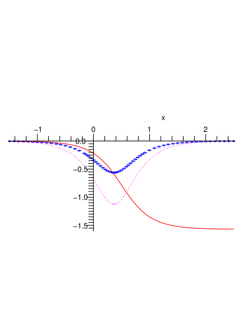3 and 4, respectively, for antisoliton and antikink solutions.

It is clear that the charge density related to this $U(1)$ current can only take significant values on those regions where the $x-$derivative of the fields $\varphi_{1,2}$ are non-vanishing. That is one expects to happen with the bag model like confinement mechanism in quantum chromodynamics (QCD). As we have seen the soliton and kink solutions of the GSG theory are localized in space, in the sense that the scalar fields interpolate between the relevant vacua in a limited region of space with a size determined by the soliton masses. The spinor $U(1)$ current gets the contributions from all the three spinor flavors. Moreover, from the equations of motion (56)-(64) one can obtain nontrivial spinor solutions different from vacuum (98) for each set of scalar field solutions $\varphi_{1},\varphi_{2}$. For example, the solution $\varphi_{1}=$soliton, $\varphi_{2}=0$ in section 2.1 implies $\phi_{1}=\varphi_{1},\,\phi_{2}=-\varphi_{1},\,\phi_{3}=0$ which substituting into the spinor equations of motion (56)-(64) will give nontrivial spinor field solutions. Therefore, the ATM model of section 3 can be considered as a multiflavor generalization of the two-dimensional hadron model proposed in [30, 31]. In the last reference a scalar field is coupled to a spinor such that the DSG kink arises as a model for hadron and the quark field is confined inside the bag.

Figure 3: 1-antisoliton and confined current $J^{\mu}$. The solid curve is the 1-antisoliton ($\frac{\beta_{0}}{4}\varphi$), the dashdotted curve is $J^{0}$ and the curve with losangles is $J^{1}$. For $t=1,\,\mu_{1}=\mu_{2}=1,d=1.5,v=0.05,\beta_{0}=0.5,\,m_{\psi}^{1}=m_{\psi}^{2}=1$, $\nu_{1}=1,\,\delta_{1}=1,\,\delta_{2}=2$.

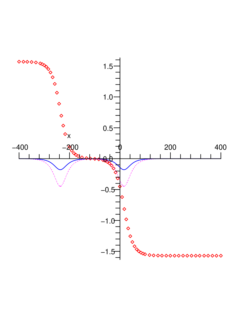
Figure 4: DSG kink solution and confined current $J^{\mu}$. The curve with losangles is the antikink ($\frac{\beta_{0}}{4}\varphi$), the dashdotted line is $J^{0}$, the solid curve is $J^{1}$. For $t=1,\,\beta_{0}=10^{8},\,m^{1,2}_{\psi}=\mu_{1}=-0.0000001,\,\,\mu_{3}:=0.001,\,\,d=2,\,\delta_{1}=\delta_{2}=1,\,\nu_{1}=1/2$.

5 Qualitons or quark solitons in two-dimensional QCD

Several properties of the ATM model deserve careful consideration in view of the relationships with two-dimensional QCD. In particular, it has been shown that the $sl(2)$ ATM model describes the low-energy spectrum of QCD₂ ($1$ flavor and $N_{c}$ colors) [19]. In the context of bosonized QCD₂ the appearance of soliton solutions that have the quantum numbers of quarks as constituent of hadrons has been considered [8]. So, one can inquire about these type of quark solitons in the context of the ATM model description of QCD₂. Since the ATM model describes the low-energy effective action in the strong coupling limit of QCQ₂, in order to disentangle the quark solitons one needs to restore, in some way, the heavy fields, i.e. the fields associated to the color degrees of freedom. For simplicity we choose the $sl(2)$ case in the following developments.

The Lagrangian of the $sl(2)$ ATM model is defined by [42, 43, 45]

$$\frac{1}{k}{\cal L}=\frac{1}{4}\partial_{\mu}\varphi\,\partial^{\mu}\varphi+i{\bar{\psi}}\gamma^{\mu}\partial_{\mu}\psi-m_{\psi}\,{\bar{\psi}}\,e^{2i\varphi\,\gamma_{5}}\,\psi,$$ (103)

where $k=\frac{\kappa}{2\pi}$,  ($\kappa\in\hbox{\sf Z}$), $\varphi$ is a real field, $m_{\psi}$ is a mass parameter, and $\psi$ is a Dirac spinor. Notice that ${\bar{\psi}}\equiv{\widetilde{\psi}}^{T}\,\gamma_{0}$. We shall take ${\widetilde{\psi}}=e_{\psi}\psi^{*}$ [43], where $e_{\psi}$ is a real dimensionless constant. The conformal version (CATM) of (103) has been constructed in [41]. The integrability properties and the reduction processes: WZNW$\rightarrow$ CATM $\rightarrow$ ATM $\rightarrow$ sine-Gordon(SG) $+$ free field, have been considered [42, 43, 45] . The $sl(n)$ ATM exhibits a generalized sine-Gordon/massive Thirring correspondence [14]. Moreover, (103) exhibits mass generation despite chiral symmetry [46] and confinement of fermions in a self-generated potential [43, 30].

The Lagrangian is invariant under $\varphi\rightarrow\varphi+n\pi$, thus the topological charge, $Q_{\mbox{topol.}}\equiv\int\,dx\,j^{0},\,j^{\mu}=\frac{1}{\pi}\epsilon^{\mu\nu}\partial_{\nu}\,\varphi$, can assume nontrivial values. A reduction is performed imposing the constraint

$$\frac{1}{2\pi}\epsilon^{\mu\nu}\partial_{\nu}\,\varphi=\frac{1}{\pi}\bar{\psi}\gamma^{\mu}\psi,$$ (104)

where $J_{\mu}=\bar{\psi}\gamma^{\mu}\psi$ is the $U(1)$ Noether current. In fact, the soliton type solutions satisfy this relationship [43].

The Eq. (104) implies $\psi^{\dagger}\psi\sim\partial_{x}\varphi$, thus the Dirac field is confined to live in regions where the field $\varphi$ is not constant. The $1(2)-$soliton(s) solution(s) for $\varphi$ and $\psi$ are of the sine-Gordon (SG) and massive Thirring (MT) types, respectively; they satisfy (104) for $|e_{\psi}|=1$, and so are solutions of the reduced model [43]. Similar results hold in $sl(n)$ ATM [34, 14].

The equivalence (104) for multisolitons describes, $\varphi=\varphi_{N}$ [$Q_{\mbox{topol}}=N\,\mbox{sign}(e_{\psi})$] and $\Psi$ $N-$solitons of the SG and MT type, respectively. Asymptotically one can write

$$\frac{1}{2\pi}\epsilon^{\mu\nu}\partial_{\nu}\,\varphi_{N}\approx\sum_{a=1}^{N}\frac{1}{\pi}\bar{\psi}_{a}\gamma^{\mu}\psi_{a},$$ (105)

where the $\psi_{a}$’s are the solutions for the individual localized lowest energy fermion states. In fact, (105) encodes the classical SG/MT correspondence [47]. Thus, the ATM model can accomodate $N_{c}=N-$fermion confined states with internal ‘color’ index $a$ [30].

In order to gain insight into the QCD₂ origin of the $\psi_{a}$ fields let us write the ‘mass term’ in the multifermion sector of ATM theory as [19]

$${\bar{\psi}}_{a}\,e^{2i\varphi\,\gamma_{5}}\,\psi^{a}=\psi^{\dagger\,a}_{L}\psi_{R\,a}\,e^{2i\varphi}+\psi^{\dagger\,a}_{R}\psi_{L\,a}\,e^{-2i\varphi}.$$ (106)

The ATM mass term in the multifermion sector, Eq. (106), must be compared to the corresponding term in the bosonized QCD₂ in order to identify the fields related to the flavor and color degrees of freedom, respectively.

Therefore the total chiral invariant Lagragian including the kinetic terms for the quark fields becomes

$$\frac{1}{k}{\cal L}=\frac{1}{4}\partial_{\mu}\varphi\,\partial^{\mu}\varphi+ie_{\psi}\sum_{a}(\bar{\psi}_{a}\gamma^{\mu}\partial_{\mu}\psi_{a}-m_{\psi}\,\bar{\psi}_{a}\,e^{2i\varphi\,\gamma_{5}}\,\psi_{a}).$$ (107)

Although the QCD color degrees of freedom have a non-abelian symmetry we use abelian bosonization techniques in order to bosonize the fermions. This will be sufficient in order to reproduce various properties of the effective QCD₂ Lagrangian in this regime as presented in ref. [8]. So, let us introduce new boson field representations of the fermion bilinears as [48]

$$i:{\bar{\psi}}_{a}\gamma^{\mu}\partial_{\mu}\psi_{a}: = -\frac{\alpha^{2}}{2\pi}(\partial_{\nu}\phi_{a})^{2}$$ (108)

$$:{\bar{\psi}}_{a}(1\pm\gamma_{5})\psi_{a}: = -\frac{c\mu}{\pi}:e^{(\pm i\alpha\phi_{a})}:,\,\,\,\,\,\,\,:{\bar{\psi}}_{a}\gamma^{\mu}\psi_{a}:\,=\,-\frac{\alpha}{\pi}\epsilon^{\mu\nu}\partial_{\nu}\phi_{a},$$ (109)

where $c=\frac{1}{2}\exp{(\gamma)}$, $\mu$ is an infrared regulator and $\alpha$ a real parameter.

In order to compare to the related QCD Lagrangian describing the regime $m_{q}>>e_{c}$ [8], which does not possess an exact chiral symmetry, we must introduce some chiral symmetry breaking terms in the Lagrangian (107). The most direct program for accomplishing this is simply to include certain chiral breaking terms in the bosonized version of the ATM$+$color model given in (107) in the form of

$${\cal L}_{bos} = \frac{k}{4}\partial_{\mu}\varphi\,\partial^{\mu}\varphi+\sum_{a}^{N_{c}}\{\frac{k\alpha^{2}e_{\psi}}{2\pi}\partial_{\mu}\phi_{a}\,\partial^{\mu}\phi_{a}+\frac{km_{\psi}c\mu e_{\psi}}{\pi}\mbox{cos}(2\varphi+2\alpha\phi_{a})-m_{a}\phi_{a}^{2}\}-$$ (110)

$$m_{0}\varphi^{2}-\sum_{a<b}m_{ab}\phi_{a}\phi_{b}-\sum_{a}m_{0a}\varphi\phi_{a}$$

Notice that we have included certain bilinear terms in the scalar fields as the symmetry breaking terms. Define the fields $\chi_{a}$ and $\Phi$ as

$$\chi_{a}\equiv\frac{2}{\beta}(\alpha\phi_{a}+\varphi);\,\,\,\,\,\Phi\equiv\frac{1}{\sqrt{2d}}(\varphi-\frac{k\beta e_{\psi}}{4\pi d}\sum_{a=1}^{N_{c}}{\chi_{a}}),\,\,\,\,d\equiv\frac{k}{4}+\frac{k\beta^{2}N_{c}e_{\psi}}{2\pi}.$$ (111)

So, providing the relationships

$$m_{a} = const,\,\,\,m_{ab}=m_{ba}=const.\,(a<b),\,\,\,m_{0a}=const,\,\,\,\,\forall a,$$ (112)

$$m_{ab} = \frac{m_{01}^{2}}{2m_{0}}-\frac{2\delta_{c}^{2}}{N_{c}},\,\,\,\,m_{a}=\frac{m_{01}^{2}}{4m_{0}}+\frac{\delta_{c}^{2}(N_{c}-1)}{N_{c}},\,\,\,\delta_{c}\equiv\frac{8e_{c}^{2}\alpha^{2}}{\beta^{2}},$$ (113)

$$e_{\psi} = \frac{-\pi m_{01}}{4\alpha m_{0}}.$$ (114)

the Lagrangian (110) becomes

$${\cal L}_{bos} = \frac{1}{2}(\partial_{\mu}\Phi)^{2}-\frac{2m_{0}}{k}(1+\frac{2N_{c}e_{\psi}}{\pi})\Phi^{2}+\sum_{a}\{\frac{1}{2}(\partial_{\mu}\chi_{a})^{2}+2M^{2}(\cos\,\beta\,\chi_{a})\}-$$ (115)

$$\frac{k^{2}e_{\psi}^{2}\beta^{2}}{8\pi^{2}d}\sum_{a<b}\partial_{\mu}\chi_{a}\partial^{\mu}\chi_{b}-2e^{2}_{c}(\frac{N_{c}-1}{N_{c}})\sum_{a}\chi_{a}^{2}+\frac{4e_{c}^{2}}{N_{c}}\sum_{a<b}\chi_{a}\chi_{b}$$

where

$$\beta^{2}=4\pi,\,\,\,\,M^{2}=\frac{c\,m_{\psi}\mu ke_{\psi}}{2\pi},\,\,\,\,e_{\psi}=\frac{N_{c}-\frac{1}{2}k\pi\pm\sqrt{N_{c}^{2}+k\pi N_{c}-2\pi k+\frac{1}{4}\pi^{2}k^{2}}}{2k(N_{c}-1)}.$$ (116)

The model (115) except the $a<b$ kinetic (the first term of the second line in (115)) and the $\Phi$ terms reproduces the QCD₂ bosonized Lagrangian (in the regime $m_{q}>>e_{c}$) presented in [8]. Notice that the $\Phi$ field completely decouples from the rest of the fields. Moreover, in the opposite limit, i.e. the strong coupling regime and large $N$ limit we can verify that this field becomes a free massless field [19].

Besides, the low-energy spectrum of QCD₂ has ben studied by means of abelian [49] and non-abelian bosonizations [50, 2]. In this limit the baryons of QCD₂ are sine-Gordon solitons [2]. In the large $N$ limit approach (weak $e$ and small $m_{q}$) the SG theory also emerges [51].

The question of confinement of the “color” degrees of freedom associated to the field $\psi$ in the ATM model by computing the string tension has been presented in [19]. In the fundamental representation of the quarks it has been taken $\frac{m_{\psi}}{4\pi}=m_{q}$ and $k=2N/\pi$. Then from (116) one has $|e_{\psi}|=\frac{\pi}{2\sqrt{N^{2}-N}}$.

Following [8] we define the baryon number as

$$B=\frac{1}{\sqrt{\pi}}\sum_{k=1}^{N_{c}}\Big{[}\chi_{k}(+\infty)-\chi_{k}(-\infty)\Big{]}$$ (117)

We seek for solutions of the field equations of motion in the static case

$$\chi^{{}^{\prime\prime}}_{a}-4M^{2}\sqrt{\pi}\,\mbox{sen}\sqrt{4\pi}\chi_{a}+\rho\sum_{b>a}^{N_{c}}\chi^{{}^{\prime\prime}}_{b}-4e_{c}^{2}\Big{(}\chi_{a}-\frac{1}{N_{c}}\sum_{b=1}^{N_{c}}\chi_{b}\Big{)}=0,$$ (118)

$$\,\,\,\,\rho\equiv[N-1+4\pi\sqrt{N(N-1)}]^{-1}.$$ (119)

Depending on the boundary conditions for the fields $\chi_{k}(\pm\infty)$ we may have certain nucleon states with $B=kN_{c},\,k\in\leavevmode\hbox{\sf Z\kern-3.99994ptZ}$ (the baryon number is normalized to be $N_{c}$ for the nucleon) or some quark solitons ($B=n,\,\,n=$integer non-multiple of $N_{c}$). These type of solutions can be discussed by analyzing the field equations for the static case [8]. In the low energy and strong coupling limit ($e_{c}>>m_{q}$) the nucleon states (baryons and multibaryon) are described by the generalized sine-Gordon solitons (see [6] and references therein), as can be inferred from the form of the eqs. of motion (118) in this limit. Whereas, the quark solitons exist for a sufficiently heavy quark $m_{q}$, but have infinite energy, corresponding to a string carrying the non-singlet color flux off to spatial infinity, i.e. they exist in the opposite limit $m_{q}>>e_{c}$. These quark soliton solutions disappear when the meson mass parameter M is reduced to become comparable to the gauge coupling strength $e_{c}$ (it has the dimension of mass in QCD2). Let us search for solutions such that $\chi_{a}(-\infty)=0$ for all $a$. Then, at $x=+\infty$ one has

$$4M^{2}\sqrt{\pi}\,\mbox{sen}\sqrt{4\pi}\chi_{a}(\infty)+4e_{c}^{2}\Big{(}\chi_{a}(\infty)-\frac{1}{N_{c}}\sum_{b=1}^{N_{c}}\chi_{b}(\infty)\Big{)}=0.$$ (120)

The eq. (120) becomes the same as the one presented in [8] describing the boundary condition at $x=+\infty$. If we assume $\chi_{a}(\infty)=\chi$ for all $a$, one has that $\chi(\infty)=\frac{1}{2}\sqrt{\pi}n$, and $B=\frac{1}{2}nN_{c}$. But, in order to have positive eigenvalues of the squared mass matrix $\frac{\partial^{2}V}{\partial{\chi_{a}}\partial{\chi_{b}}}$, we must have even $n$, and thus integer baryon number $B=kN_{c}$ (baryons and multibaryons).

Following [8], in the search for quark solitons let us first concentrate on the case $N_{c}=2$. Then, eq. (120) can be written as

$$\mbox{sin}\sqrt{4\pi}\chi_{1}(\infty) = -\epsilon\sqrt{\pi}[\chi_{1}(\infty)-\chi_{2}(\infty)],$$ (121)

$$\mbox{sin}\sqrt{4\pi}\chi_{2}(\infty) = -\epsilon\sqrt{\pi}[\chi_{2}(\infty)-\chi_{1}(\infty)],$$ (122)

where $\epsilon=\frac{e_{c}^{2}}{2\pi M^{2}}$. We may have non-baryonic solitons with $B=n$ for odd values of $n$ (the quarks correspond to $n=1$). For $\epsilon<<1$ we can find a series of solutions with positive second derivative matrix. This solution satisfies

$$\chi_{2}(\infty)=-\chi_{2}(\infty)+n\sqrt{\pi},$$ (123)

which together with (121)-(122) provides

$$\mbox{sin}\sqrt{4\pi}\chi_{1}=-\epsilon(\sqrt{4\pi}\chi_{1}-n\pi).$$ (124)

Let us define $\xi=\sqrt{4\pi}[\chi(\infty)-\frac{1}{2}n\sqrt{\pi}]$, then one has that the solutions are

$$\xi_{l}=\left\{\begin{array}[]{ll}(\pi-\epsilon)(2l)&\mbox{for }n\,\,\mbox{even}\\ (\pi-\epsilon)(2l+1)&\mbox{for }n\,\,\mbox{odd}\end{array}\right.,$$ (127)

in the limit where $(l\epsilon<<\frac{1}{4})$. The solutions (127) correspond to excitations of “colored” states and have infinite energy, with classical string tension

$$T\approx\left\{\begin{array}[]{ll}\pi\,e_{c}^{2}\,(2l)^{2}&\mbox{for }n\,\,\mbox{even}\\ \pi\,e_{c}^{2}\,(2l+1)^{2}&\mbox{for }n\,\,\mbox{odd}\end{array}\right..$$ (130)

The single constituent quark soliton corresponds to $n=1,(2l+1)=1$. Thus, we have shown that QCD₂ has quark soliton solutions if the quark mass is sufficiently large. These quark solitons disappear when the quark mass $m_{q}$ is reduced until the meson mass M becomes comparable to the dimensional gauge coupling strength $e_{c}$. The above picture can be directly generalized for any $N_{c}$, see more details in [8].

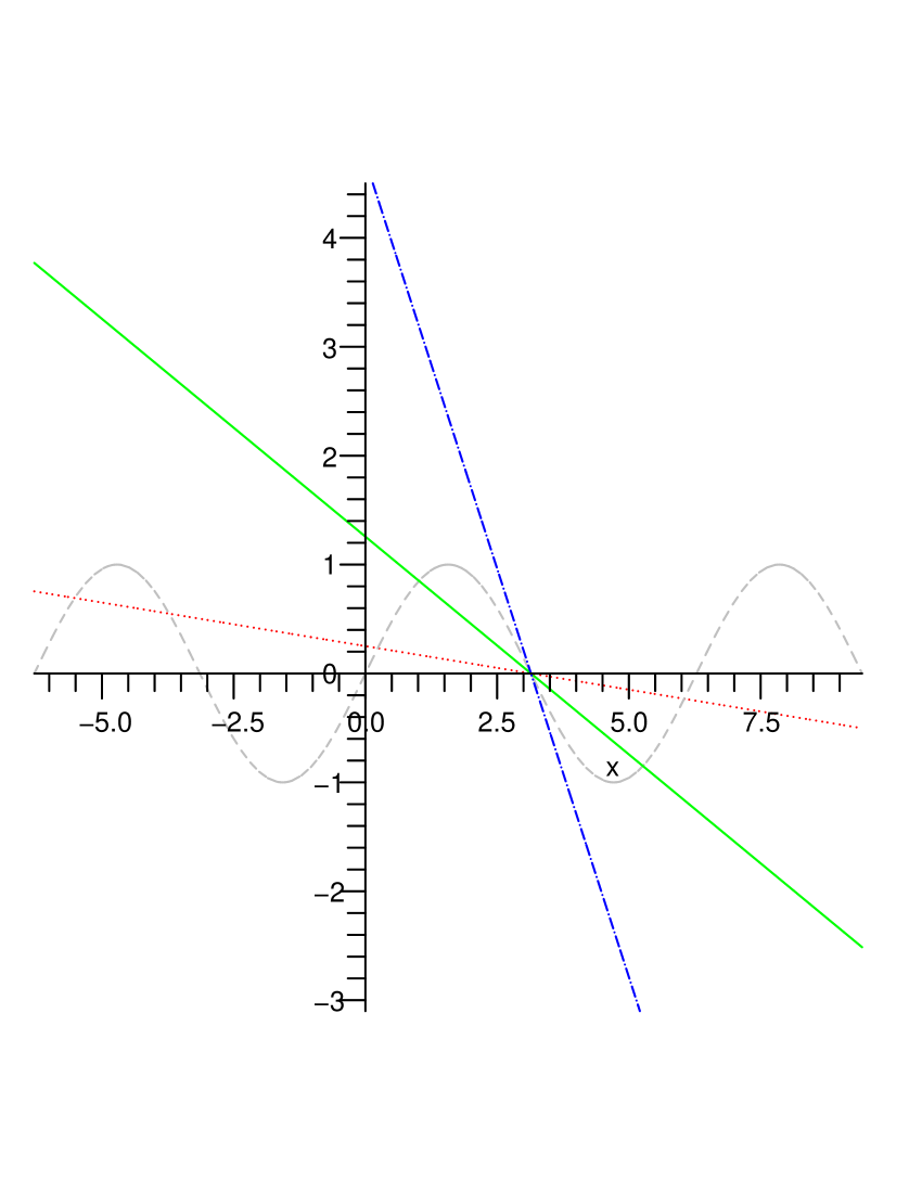
Figure 5: The axis is defined as $x\equiv\sqrt{4\pi}\chi_{1}(\infty)$. Comparison of the left-and right-hand sides of the soliton eq. (124), corresponding to a quark soliton with $n=1$, for $\epsilon=0.08$ (dotted line) and $\epsilon=0.4$ (solid line). There are no solutions for $\epsilon>1$ (dot-dashed line, drawn for $\epsilon=1.5$).

6 Discussion

The generalized sine-Gordon model GSG (10)-(11) provides a variety of solitons, kinks and bounce type solutions. The appearance of the non-integrable double sine-Gordon model as a sub-model of the GSG model suggests that this model is a non-integrable theory for the arbitrary set of values of the parameter space. However, a subset of values in parameter space determine some reduced sub-models which are integrable, e.g. the sine-Gordon submodels of subsections 2.1, 2.2 and 2.3.

In connection to the ATM spinors it was suggested that they are confined inside the GSG solitons and kinks since the gauge fixing procedure does not alter the $U(1)$ and topological currents equivalence (75). Then, in order to observe the bag model confinement mechanism it is not necessary to solve for the spinor fields since it naturally arises from the currents equivalence relation. In this way our model presents a bag model like confinement mechanism as is expected in QCD.

The (generalized) massive Thirring model (GMT) is bosonized to the GSG model [17], therefore, in view of the solitons and kinks found above as solutions of the GSG model we expect that the spectrum of the GMT model will contain $4$ solitons and their relevant anti-solitons, as well as the kink and antikink excitations. The GMT Lagrangian describes three flavor massive spinors with current-current interactions among themselves. So, the total number of solitons which appear in the bosonized sector suggests that the additional soliton (fermion) is formed due to the interactions between the currents in the GMT sector. However, in subsection 2.3 the soliton masses $M_{3}$ and $M_{4}$ become the same for the case $\mu_{1}=\mu_{2}$, consequently, for this case we have just three solitons in the GSG spectrum, i.e., the ones with masses $M_{1}$, $M_{2}$ (subsections 2.1-2.2 ) and $M_{3}=M_{4}$ (subsection 2.3), which will correspond in this case to each fermion flavor of the GMT model. Moreover, the $sl(3)$ GSG model potential (6) has the same structure as the effective Lagrangian of the massive Schwinger model with $N_{f}=3$ fermions, for a convenient value of the vacuum angle $\theta$. The multiflavor Schwinger model resembles with four-dimensional QCD in many respects (see e.g. [52] and references therein).

The $sl(n)$ ATM models may be relevant in the construction of the low-energy effective theories of multiflavor QCD₂ with the dynamical fermions in the fundamental and adjoint representations. Notice that in these models the Noether and topological currents and the generalized sine-Gordon/massive Thirring models equivalences take place at the classical [15, 42] and quantum mechanical level [17, 43].

The interest in baryons with exotic quantum numbers has recently been stimulated by various reports of baryons composed by four quarks and an antiquark. The existence of these baryons cannot yet be regarded as confirmed, however, reports of their existence have stimulated new investigations about baryon structure (see e.g. [53] and references therein). Recently, the spectrum of exotic baryons in QCD₂, with $SU(N_{f})$ flavor symmetry, has been discussed providing strong support to the chiral-soliton picture for the structure of normal and exotic baryons in four dimensions [6, 54]. The new puzzles in non-perturbative QCD are related to systems with unequal quark masses, so the QCD₂ calculation must take into account the $SU(N_{f})$-breaking mass effects, i.e. for $N_{f}=3$ it must be $m_{s}\neq m_{u,d}$. So, in view of our results above, the properties of the GSG and the ATM theories may find some applications in the study of mass splitting of baryons in QCD₂ and the understanding of the internal structure of baryons. Regarding this line of research, it has been shown that the GSG model describes the low-energy spectrum of normal and exotic baryons in QCD$2$ with unequal quark mass parameters [6].

Finally, we have considered the quark soliton (qualiton) solutions of QCD₂ in the regime $e_{c}<<m_{q}$. In this context the role played by the sl(2) ATM model is clarified. In fact, the qualitons arise if the color degrees of freedom are restored by coupling them to the Toda field and convenient boundary conditions are imposed on the fields. So, we have shown that the sl(2) ATM model becomes a low-energy effective lagrangian describing the quark confinement mechanism in QCD₂. The equivalence between the Noether and topological currents (104) is a crucial property of the ATM model in order to provide the confinement mechanism. This picture can be directly generalized to any number of flavors $N_{f}$ since a relationship analog to (104) holds in that case, e.g. the $N_{f}=3$ case is presented in (75).

Acknowledgements

HB thanks the Physics Department-UFMT (Cuiabá) and IMPA (Rio de Janeiro) for hospitality. HLC thanks FAPESP for support.

Appendix A The zero-curvature formulation of the ATM model

We summarize the zero-curvature formulation of the $sl(3)$ ATM model [14, 15, 34]. Consider the zero curvature condition

$$\partial_{+}A_{-}-\partial_{-}A_{+}+[A_{+},A_{-}]=0.$$ (131)

The potentials take the form

$$A_{+}=-BF^{+}B^{-1},\quad A_{-}=-\partial_{-}BB^{-1}+F^{-},\qquad$$ (132)

with

$$F^{+}\,=\,F_{1}^{+}+F_{2}^{+},\,\,\,\,\,\,F^{-}\,=\,F_{1}^{-}+F_{2}^{-},$$ (133)

where $B$ and $F_{i}^{\pm}$ contain the fields of the model

$$F_{1}^{+} = \sqrt{im^{1}_{\psi}}\psi_{R}^{1}E_{\alpha_{1}}^{0}+\sqrt{im^{2}_{\psi}}\psi_{R}^{2}E_{\alpha_{2}}^{0}+\sqrt{im^{3}_{\psi}}\widetilde{\psi}_{R}^{3}E_{-\alpha_{3}}^{1},$$ (134)

$$F_{2}^{+} = \sqrt{im^{3}_{\psi}}\psi_{R}^{3}E_{\alpha_{3}}^{0}+\sqrt{im^{1}_{\psi}}\widetilde{\psi}_{R}^{1}E_{-\alpha_{1}}^{1}+\sqrt{im^{2}_{\psi}}\widetilde{\psi}_{R}^{2}E_{-\alpha_{2}}^{1},$$ (135)

$$F_{1}^{-} = \sqrt{im^{3}_{\psi}}\psi_{L}^{3}E_{\alpha_{3}}^{-1}+\sqrt{im^{1}_{\psi}}\widetilde{\psi}_{L}^{1}E_{-\alpha_{1}}^{0}+\sqrt{im^{2}_{\psi}}\widetilde{\psi}_{L}^{2}E_{-\alpha_{2}}^{0},$$ (136)

$$F_{2}^{-} = \sqrt{im^{1}_{\psi}}\psi_{L}^{1}E_{\alpha_{1}}^{-1}+\sqrt{im^{2}_{\psi}}\psi_{L}^{2}E_{\alpha_{2}}^{-1}+\sqrt{im^{3}_{\psi}}\widetilde{\psi}_{L}^{3}E_{-\alpha_{3}}^{0},$$ (137)

$$B = e^{i\theta_{1}H^{0}_{1}+i\theta_{2}H^{0}_{2}}\,e^{\widetilde{\nu}C}\,e^{\eta Q_{ppal}}\equiv b\,e^{\widetilde{\nu}C}\,e^{\eta Q_{ppal}}.$$ (138)

$E_{\alpha_{i}}^{n},H^{n}_{1},H^{n}_{2}$ and $C$ ($i=1,2,3;\,n=0,\pm 1$) are some generators of $sl(3)^{(1)}$; $Q_{ppal}$ being the principal gradation operator. The commutation relations for an affine Lie algebra in the Chevalley basis are

$$\left[\emph{H}_{a}^{m},\emph{H}_{b}^{n}\right]=mC\frac{2}{\alpha_{a}^{2}}K_{ab}\delta_{m+n,0}$$ (139)

$$\left[\emph{H}_{a}^{m},E_{\pm\alpha}^{n}\right]=\pm K_{\alpha a}E_{\pm\alpha}^{m+n}$$ (140)

$$\left[E_{\alpha}^{m},E_{-\alpha}^{n}\right]=\sum_{a=1}^{r}l_{a}^{\alpha}\emph{H}_{a}^{m+n}+\frac{2}{\alpha^{2}}mC\delta_{m+n,0}$$ (141)

$$\left[E_{\alpha}^{m},E_{\beta}^{n}\right]=\varepsilon(\alpha,\beta)E_{\alpha+\beta}^{m+n};\qquad\mbox{if }\alpha+\beta\mbox{ is a root \qquad}$$ (142)

$$\left[D,E_{\alpha}^{n}\right]=nE_{\alpha}^{n},\qquad\left[D,\emph{H}_{a}^{n}\right]=n\emph{H}_{a}^{n}.$$ (143)

where $K_{\alpha a}=2\alpha.\alpha_{a}/\alpha_{a}^{2}=n_{b}^{\alpha}K_{ba}$, with $n_{a}^{\alpha}$ and $l_{a}^{\alpha}$ being the integers in the expansions $\alpha=n_{a}^{\alpha}\alpha_{a}$ and $\alpha/\alpha^{2}=l_{a}^{\alpha}\alpha_{a}/\alpha_{a}^{2}$, and $\varepsilon(\alpha,\beta)$ the relevant structure constants.

Take $K_{11}=K_{22}=2$ and $K_{12}=K_{21}=-1$ as the Cartan matrix elements of the simple Lie algebra $sl(3)$. Denoting by $\alpha_{1}$ and $\alpha_{2}$ the simple roots and the highest one by $\psi(=\alpha_{1}+\alpha_{2})$, one has $l_{a}^{\psi}=1(a=1,2)$, and $K_{\psi 1}=K_{\psi 2}=1$. Take $\varepsilon(\alpha,\beta)=-\varepsilon(-\alpha,-\beta),\,\,\varepsilon_{1,2}\equiv\varepsilon(\alpha_{1},\alpha_{2})=1,\,\,\varepsilon_{-1,3}\equiv\varepsilon(-\alpha_{1},\psi)=1\,\,\mbox{and}\,\,\,\varepsilon_{-2,3}\equiv\varepsilon(-\alpha_{2},\psi)=-1$.

One has $Q_{ppal}\equiv\sum_{a=1}^{2}{\bf s}_{a}\lambda^{v}_{a}.H+3D$, where $\lambda^{v}_{a}$ are the fundamental co-weights of $sl(3)$, and the principal gradation vector is ${\bf s}=(1,1,1)$ [55].