New lattice action for heavy quarks

Abstract

We extend the Fermilab method for heavy quarks to include interactions of dimensions 6 and 7 in the action. There are, in general, many new interactions, but we carry out the calculations needed to match the lattice action to continuum QCD at the tree level, finding six non-zero couplings. Using the heavy-quark theory of cutoff effects, we estimate how large the remaining discretization errors are. We find that our tree-level matching, augmented with one-loop matching of the dimension-five interactions, can bring these errors below 1%, at currently available lattice spacings.

I Introduction

An important application of lattice gauge theory is to calculate hadronic matrix elements relevant to experiments in flavor physics. With recent advances in lattice calculations with $n_{f}=2+1$ flavors of dynamical quarks Bernard:2002bk ; Aubin:2004ej ; Aubin:2005ar ; Allison:2004be , we now have an exciting prospect of genuine QCD calculations. To match the experimental uncertainty, available now or in the short term, it is essential to control all other sources of theoretical uncertainty as well as possible. An attractive target is to reduce the uncertainty, from any given source, to 1–2%. This target will be hard to hit if one relies on increases in computer power alone: methodological improvements are needed too.

Many of the important processes are electroweak transitions of heavy charmed or $b$-flavored quarks. A particular challenge stems from heavy-quark discretization effects, because $m_{Q}a\not\ll 1$. The key to meeting the challenge is to observe that heavy quarks are non-relativistic in the rest frame of the containing hadron Eichten:1987xu ; Lepage:1987gg . The scale of the heavy-quark mass, $m_{Q}$, can (and should) be separated from the soft scales inside the hadron and treated with an effective field theory instead of computer simulation. Even so, at available lattice spacings Bernard:2002bk , many calculations of $D$-meson ($B$-meson) properties suffer from a discretization error of around 7% (5%) Aubin:2004ej ; Aubin:2005ar . Thus, it makes sense to develop a more accurate discretization.

In this paper we extend the accuracy of the “Fermilab” method for heavy quarks El-Khadra:1996mp to include in the lattice action all interactions of dimension six. We also include certain interactions of dimension seven. Because heavy quarks are non-relativistic, they are commensurate with related dimension-6 terms, in the power counting of heavy-quark effective theory (HQET) for heavy-light hadrons Eichten:1987xu or non-relativistic QCD (NRQCD) for quarkonium Lepage:1987gg .

The Fermilab method starts with Wilson fermions Wilson:1975hf and the clover action Sheikholeslami:1985ij . With these actions lattice spacing effects are bounded for large $m_{Q}a$, thanks to heavy-quark symmetry. They can be reduced systematically by allowing an asymmetry between spatial and temporal interactions. Asymmetry in the lattice action compensates for the non-relativistic kinematics, enabling a relativistic description through the Symanzik effective field theory Symanzik:1979ph . Alternatively, one may interpret Wilson fermions non-relativistically from the outset El-Khadra:1996mp , and set up the improvement program matching lattice gauge theory and continuum QCD to each other through HQET and NRQCD Kronfeld:2000ck ; Harada:2001fi . The Symanzik description makes it possible to design a lattice action that behaves smoothly as $m_{Q}a\to 0$, converging to the universal continuum limit. The HQET description, on the other hand, makes semiquantitative estimates of discretization errors more transparent.

The new action introduced below has nineteen bilinear interactions beyond those of the asymmetric version of the clover action, as well as many four-quark interactions. Several of these couplings are redundant, and many more vanish when matching to continuum QCD at the tree level. We study semiquantitatively how many of the new operators are needed to achieve 1–2% accuracy. We find, in the end, that only six new interactions are essential for such accuracy. The action is designed with some flexibility, so that one may choose the computationally least costly version of the action.

This paper is organized as follows. Section II considers the description of lattice gauge theory via continuum effective field theories. Then, in some detail, we identify a full set of operators describing heavy-quark discretization effects. We then determine how many of these are redundant, and which redundant directions should be used to preserve the good high-mass behavior. We have two goals in this analysis. One is to design the new, more highly improved, action; for this step a Symanzik-like description is more helpful, and the resulting action is given in Sec. III. The other is to estimate the discretization errors of the new action; here the HQET and NRQCD descriptions are more useful. To make error estimates, and to use the new action in numerical work, we need matching calculations; they are in Sec. IV. Our error estimates are in Sec. V. Section VI concludes. Some of the material is technical and appears in appendices: Feynman rules needed for the matching calculation are in Appendix A; some details of the Compton scattering amplitude used for matching are in Appendix B; a discussion of improvement of the gauge action on anisotropic lattices (which one needs only if the heavy quarks are not quenched) is in Appendix C. Some of these results have been reported earlier Oktay:2002mj .

II Effective Field Theory

In this section we discuss how to understand and control discretization effects using effective field theories. We start with a brief overview, focusing on issues that arise for heavy quarks, those with mass $m_{Q}\gg\Lambda$. For more details, the reader may consult earlier work El-Khadra:1996mp ; Kronfeld:2000ck ; Harada:2001fi ; Aoki:2001ra ; Christ:2006us or a pedagogical review Kronfeld:2002pi . Here we catalog all interactions of dimension 6 and also certain interactions of dimension 7 that, for heavy quarks, are of comparable size when $m_{Q}a\not\ll 1$.

II.1 Overview

Cutoff effects in lattice field theories are most elegantly studied with continuum effective field theories. The idea originated with Symanzik Symanzik:1979ph and was extended to gluons and light quarks by Weisz and collaborators Weisz:1982zw ; Weisz:1983bn ; Luscher:1984xn ; Sheikholeslami:1985ij . One develops a relationship

$${\cal L}_{\mathrm{lat}}\doteq{\cal L}_{\mathrm{Sym}},$$ (1)

where $\doteq$ means that the two Lagrangians generate the same on-shell spectrum and matrix elements. The lattice itself regulates the ultraviolet behavior of the underlying (lattice) theory ${\cal L}_{\mathrm{lat}}$. On the other hand, a continuum scheme, which does not need to be specified in detail, regulates (and renormalizes) the ultraviolet behavior of the effective theory ${\cal L}_{\mathrm{Sym}}$.

In lattice QCD (with Wilson fermions), the local effective Lagrangian (LE${\cal L}$) is

$${\cal L}_{\mathrm{Sym}}=\frac{1}{2g^{2}}\mathop{\mathrm{tr}}[F_{\mu\nu}F^{\mu\nu}]-\sum_{f}\bar{q}_{f}({D\kern-6.49994pt/}+m_{f})q_{f}+\sum_{i}a^{\dim{\cal L}_{i}-4}K_{i}(g^{2},ma;c_{j};\mu a){\cal L}_{i},$$ (2)

where $g^{2}$ and $m_{f}$ are the gauge coupling and quark mass (of flavor $f$), renormalized at scale $\mu\lesssim a^{-1}$. The (continuum) QCD Lagrangian appears as the first two terms. The sum consists of higher dimension operators ${\cal L}_{i}$, multiplied by short-distance coefficients $K_{i}$. These terms describe cutoff effects. The short-distance coefficients depend on the renormalization point and on the couplings, including couplings $c_{j}$ of improvement terms in ${\cal L}_{\mathrm{lat}}$. Equation (2) is fairly well-established to all orders in perturbation theory Luscher:1998pe ; Adams:2007gh and believed to hold non-perturbatively as well. If $a$ is small enough, the terms ${\cal L}_{i}$ may be treated as operator insertions, leading to a description of lattice gauge theory as “QCD + small corrections”.

In heavy-quark physics $m_{Q}\gg\Lambda$, where $\Lambda$ is the QCD scale, so one is led to consider what happens when $m_{Q}a\not\ll 1$. The short-distance coefficients depend explicitly on the mass. Time derivatives of heavy-quark or heavy-antiquark fields in the ${\cal L}_{i}$ also generate mass dependence of observables. With field redefinitions—or, equivalently, with the equations of motion—these time derivatives can be eliminated. Focusing on a single heavy flavor $Q$, the result of these manipulations is El-Khadra:1996mp ; Aoki:2001ra ; Christ:2006us

$${\cal L}_{\mathrm{Sym}}=\cdots-\bar{Q}\left(\gamma_{4}D_{4}+m_{1}+\sqrt{\frac{m_{1}}{m_{2}}}\bm{\gamma}\cdot\bm{D}\right)Q+\sum_{i}a^{\dim\bar{\cal L}_{i}-4}\bar{K}_{i}(g^{2},m_{2}a;\mu a)\bar{\cal L}_{i},$$ (3)

where the ellipsis denotes the unaltered LE${\cal L}$ for gluons and light quarks. By construction the $\bar{\cal L}_{i}$ do not have any time derivatives acting on quarks or antiquarks.

The advantage of Eq. (3) is that all dependence on the heavy-quark mass is in the short-distance coefficients $m_{1}$, $\sqrt{m_{1}/m_{2}}$, and $\bar{K}_{i}(m_{2}a)$. Matrix elements of the $\bar{\cal L}_{i}$ generate soft scales. The heavy-quark symmetry of Wilson quarks (with either the Wilson Wilson:1975hf or Sheikholeslami-Wohlert Sheikholeslami:1985ij actions) guarantees that the coefficients $\bar{K}_{i}(m_{2}a)$ are bounded for all $m_{2}a$. This feature can be preserved by improving the lattice Lagrangian with discretizations of the $\bar{\cal L}_{i}$, thereby avoiding higher time derivatives El-Khadra:1996mp ; Kronfeld:2000ck . For such improved actions, Eq. (3) neatly isolates the potentially most serious problem of heavy quarks into the deviation of the coefficient $\sqrt{m_{1}/m_{2}}$ from $1$.

Fortunately, the problem can be circumvented in two simple ways. One is a Wilson-like action with two hopping parameters El-Khadra:1996mp , tuned so that $m_{1}=m_{2}$. Then Eq. (3) once again takes the form “QCD + small corrections”. The new lattice action introduced in Sec. III has two hopping parameters for this reason.

Another solution is to interpret Wilson fermions in a non-relativistic framework. One can replace the Symanzik description with one using a non-relativistic effective field theory for the quarks (and antiquarks) Kronfeld:2000ck . For the leading $\bar{Q}$-$Q$ term in Eq. (3)

$$\bar{Q}\left(\gamma_{4}D_{4}+m_{1}+\sqrt{\frac{m_{1}}{m_{2}}}\bm{\gamma}\cdot\bm{D}\right)Q\doteq\bar{h}^{(+)}\left(D_{4}+m_{1}-\frac{\bm{D}^{2}+z_{B}(m_{2}a,\mu a)i\bm{\Sigma}\cdot\bm{B}}{2m_{2}}\right)h^{(+)}+\cdots$$ (4)

where $z_{B}$ is a matching coefficient, and $h^{(+)}$ is a heavy-quark field satisfying $h^{(+)}=+\gamma_{4}h^{(+)}$. Another set of terms appears for the antiquark, with field $h^{(-)}$ satisfying $h^{(-)}=-\gamma_{4}h^{(-)}$. The non-relativistic effective theory conserves heavy quarks and heavy antiquarks separately. As a consequence, the rest mass $m_{1}$ has no effect on mass splittings and matrix elements. For lattice gauge theory this implies that the bare quark mass (or hopping parameter) should not be adjusted via $m_{1}$. Instead, the bare mass should be adjusted to normalize the kinetic energy $\bm{D}^{2}/2m_{2}$.

One can develop the non-relativistic effective theory for the lattice artifacts $\bar{\cal L}_{i}$ by using heavy-quark fields instead of Dirac quark fields Kronfeld:2000ck . Higher-dimension operators in the heavy-quark theory receive contributions from the expansions of Eq. (4) and of the $\bar{\cal L}_{i}$. Coalescing the coefficients of like operators obtains a description of lattice gauge theory with heavy quarks

$${\cal L}_{\mathrm{lat}}\doteq\cdots-\bar{h}^{(+)}(D_{4}+m_{1})h^{(+)}+\sum_{i}{\cal C}_{i}^{\mathrm{lat}}(g^{2},m_{2};m_{2}a,c_{j};\mu/m_{2}){\cal O}_{i},$$ (5)

where the operators ${\cal O}_{i}$ on the right-hand side are those of a (continuum) heavy-quark effective theory, of dimension 5 and higher, built out of heavy-quark fields $h^{(\pm)}$, gluons, and light quarks. (The leading ellipsis denotes term for the gluons and light quarks only.) The ${\cal C}_{i}$ are short-distance coefficients, which depend on $g^{2}$, the heavy-quark mass, the ratio of short distances $m_{2}a$, and also all couplings $c_{j}$ in the lattice action. The logic and structure is the same as the non-relativistic description of QCD,

$${\cal L}_{\mathrm{QCD}}\doteq\cdots-\bar{h}^{(+)}(D_{4}+m_{Q})h^{(+)}+\sum_{i}{\cal C}_{i}^{\mathrm{cont}}(g^{2},m_{Q};\mu/m_{Q}){\cal O}_{i}.$$ (6)

Thus, improvement of lattice gauge theory is attained by adjusting couplings $c_{j}$ until ${\cal C}_{i}^{\mathrm{lat}}(c_{j})-{\cal C}_{i}^{\mathrm{cont}}$ vanishes (identically, or perhaps to some accuracy) for the first several ${\cal O}_{i}$.

It does not matter whether one carries out the improvement program by adjusting $\bar{K}_{i}(c_{j})=0$ or ${\cal C}_{i}^{\mathrm{lat}}(c_{j})={\cal C}_{i}^{\mathrm{cont}}$ Harada:2001fi . The results for the $c_{j}$ are the same, provided one identifies $m_{Q}$ with $m_{2}$. The matching assumes that $\bm{p}a\ll 1$, but at the same time $m_{2}a\not\ll 1$. One is thus led to non-relativistic kinematics ($\bm{p}/m_{2}\ll 1$) in the matching calculation, where both descriptions—Eqs. (3) and (5)—are valid. Kinematics are encoded into the operators $\bar{\cal L}_{i}$ or ${\cal O}_{i}$ and are not transferred to the short-distance coefficients. Hence, kinematics cannot influence matching conditions on the $c_{j}$. In particular, when indeed $m_{2}a\ll 1$ (which may be impractical, but is conceivable theoretically) relativistic kinematics ($\bm{p}\sim m_{2}$) are possible, and it follows from the Symanzik effective field theory that the solution of $\bar{K}_{i}(c_{j})=0$ yields the same $c_{j}$ for both relativistic and non-relativistic kinematics.

II.2 Quark bilinears in the LE${\cal L}$

In the rest of this section we construct the LE${\cal L}$ appropriate to heavy quarks. The two main steps are first to list all of the ${\cal L}_{i}$ that can appear, and second to decide which should be considered redundant. In part it is a generalization of the dimension-6 analysis of Ref. Sheikholeslami:1985ij to the case without axis-interchange symmetry. At dimension 6 there are quark bilinears, four-quark interactions, and interactions that contain only the gauge field. We shall start with the bilinears and turn to the others further below. In each case, we first consider complete lists of operators, and then consider which can be chosen to be redundant.

Table 1 contains a list of all quark bilinears through dimension 6 that can appear in the effective Lagrangian.

Table 1: Bilinear interactions that could appear in the Symanzik LE${\cal L}$ through dimension 6.

Dim	With axis-interchange symmetry		Without axis-interchange symmetry		HQET $\lambda^{s}$	NRQCD $\upsilon^{t}$
3	$\bar{q}q$		$\bar{Q}Q$
4	$\bar{q}{D\kern-6.49994pt/}q$		$\bar{Q}(\gamma_{4}D_{4}+m_{1})Q$		$1$	$\upsilon^{2}$
			$\bar{Q}\bm{\gamma}\cdot\bm{D}Q$		$\lambda$	$\upsilon^{2}$
5	$\bar{q}D^{2}q$	$\varepsilon_{1}$	$\bar{Q}D_{4}^{2}Q$	$\varepsilon_{1}$
			$\bar{Q}\bm{D}^{2}Q$	$\delta_{1}$	$\lambda$	$\upsilon^{2}$
	$-{\textstyle\frac{i}{2}}\bar{q}\sigma_{\mu\nu}F_{\mu\nu}q$		$\bar{Q}i\bm{\Sigma}\cdot\bm{B}Q$		$\lambda$	$\upsilon^{4}$
			$\bar{Q}\bm{\alpha}\cdot\bm{E}Q$		$\lambda^{2}$	$\upsilon^{4}$
6	$\bar{q}\gamma_{\mu}D_{\mu}^{3}q$		$\bar{Q}\gamma_{i}D_{i}^{3}Q$		$\lambda^{3}$	$\upsilon^{4}$
	$\bar{q}\{{D\kern-6.49994pt/},D^{2}\}q$	$\varepsilon_{2}$	$\bar{Q}\gamma_{4}D_{4}^{3}Q$	$\varepsilon_{2}$
			$\bar{Q}\{\gamma_{4}D_{4},\bm{D}^{2}\}Q$	$\delta_{2}$
			$\bar{Q}\{D_{4}^{2},\bm{\gamma}\cdot\bm{D}\}Q$	$\vartheta_{2}$
			$\bar{Q}\{\bm{\gamma}\cdot\bm{D},\bm{D}^{2}\}Q$		$\lambda^{3}$	$\upsilon^{4}$
	$-{\textstyle\frac{i}{2}}\bar{q}\{{D\kern-6.49994pt/},\sigma_{\mu\nu}F_{\mu\nu}\}q$	$\varepsilon_{F}$	$\bar{Q}\{\bm{\gamma}\cdot\bm{D},\bm{\alpha}\cdot\bm{E}\}Q$	$\varepsilon_{F}$	$\lambda^{2}$	$\upsilon^{4}$
			$\bar{Q}\{\gamma_{4}D_{4},i\bm{\Sigma}\cdot\bm{B}\}Q$	$\delta_{B}$
			$\bar{Q}\{\bm{\gamma}\cdot\bm{D},i\bm{\Sigma}\cdot\bm{B}\}Q$		$\lambda^{3}$	$\upsilon^{6}$
			$\bar{Q}[D_{4},\bm{\gamma}\cdot\bm{E}]Q$		$\lambda^{3}$	$\upsilon^{6}$
	$\bar{q}[D_{\mu},F_{\mu\nu}]\gamma_{\nu}q$		$\bar{Q}\gamma_{4}(\bm{D}\cdot\bm{E}-\bm{E}\cdot\bm{D})Q$		$\lambda^{2}$	$\upsilon^{4}$
			$\bar{Q}\bm{\gamma}\cdot(\bm{D}\times\bm{B}+\bm{B}\times\bm{D})Q$		$\lambda^{3}$	$\upsilon^{6}$

The second column contains interactions that respect axis-interchange symmetry; the fourth column contains the extension to the case without axis-interchange symmetry. The meaning of the other columns is explained below. Covariant derivatives act on all fields to the right,

$$D_{\mu}FQ=(\partial_{\mu}F+[A_{\mu},F])Q+F\,D_{\mu}Q.$$ (7)

This notation is convenient for the interactions with commutators and anti-commutators. To arrive at the lists we exploit identities such as

$${D\kern-6.49994pt/}^{2} = D^{2}-{\textstyle\frac{i}{2}}\sigma_{\mu\nu}F_{\mu\nu},$$ (8)

$$2\gamma_{4}D_{4}\bm{\gamma}\cdot\bm{D}\gamma_{4}D_{4} = \{\gamma_{4}D_{4},\bm{\alpha}\cdot\bm{E}\}-\{D_{4}^{2},\bm{\gamma}\cdot\bm{D}\},$$ (9)

$$2\bm{\gamma}\cdot\bm{D}\gamma_{4}D_{4}\bm{\gamma}\cdot\bm{D} = \{\bm{\gamma}\cdot\bm{D},\bm{\alpha}\cdot\bm{E}\}-\{\gamma_{4}D_{4},(\bm{\gamma}\cdot\bm{D})^{2}\}.$$ (10)

Some interactions are omitted, because the underlying lattice gauge theory is invariant under cubic rotations, spatial inversion, time reflection, and charge conjugation.

The fourth column is arranged so that its entries are part of the corresponding interactions in the second column. It is easy to show that the list is complete, by writing out all independent ways to have three covariant derivatives, expressing the $\bm{E}$ and $\bm{B}$ fields as anti-commutators of covariant derivatives. One finds 11 possibilities, and then one can use identities to manipulate this list to that given in the fourth column of Table 1.

The LE${\cal L}$ contains several redundant directions. The equation of motion of the leading LE${\cal L}$ plays a key role in specifying which operator insertions may be considered redundant. Let us assume, for the moment, that $m_{1}=m_{2}$, so that the equation of motion in the Symanzik LE${\cal L}$ is the Dirac equation. Below we shall use the non-relativistic effective field theory to address the case $m_{1}\neq m_{2}$.

The quark fields are integration variables in a functional integral, so an equally valid description is obtained by changing variables

$$Q \mapsto e^{J}Q,$$ (11)

$$\bar{Q} \mapsto \bar{Q}e^{\bar{J}},$$ (12)

where

$$J=a\varepsilon_{1}({D\kern-6.49994pt/}+m) + a\delta_{1}\bm{\gamma}\cdot\bm{D}+a^{2}\varepsilon_{2}({D\kern-6.49994pt/}+m)^{2}-a^{2}{\textstyle\frac{1}{2}}\varepsilon_{F}i\sigma_{\mu\nu}F_{\mu\nu}+a^{2}\delta_{2}(\bm{\gamma}\cdot\bm{D})^{2}$$ (13)

$$+ a^{2}\delta_{B}i\bm{\Sigma}\cdot\bm{B}+a^{2}\vartheta_{2}[\gamma_{4}D_{4},\bm{\gamma}\cdot\bm{D}]$$

and similarly for $\bar{J}$ with separate parameters $\bar{\varepsilon}_{i}$, $\bar{\delta}_{i}$, and $\bar{\vartheta}_{i}$. If the $\delta$ parameters (and $\vartheta_{2}$, $\bar{\vartheta}_{2}$) vanish, then $J$ and $\bar{J}$ preserve invariance under interchange of all four axes.

One can propagate the change of variables to the LE${\cal L}$, and trace which coefficients of dimensions 5 and 6 are shifted by amounts proportional to the parameters in $J$ and $\bar{J}$. To avoid generating terms that violate charge conjugation one chooses $\bar{\varepsilon}_{i}=+\varepsilon_{i}$, $\bar{\delta}_{i}=+\delta_{i}$, $\bar{\vartheta}_{2}=-\vartheta_{2}$. We then see that there are two redundant directions at dimension 5, and five at dimension 6. That means that two couplings in the dimension-5 lattice action may be set by convenience, and five in the dimension-6 lattice action. The third and fifth columns show the correspondence between parameters in the change of variables and the interactions that we choose to be redundant. As expected from general arguments El-Khadra:1996mp ; Aoki:2001ra ; Christ:2006us , all interactions in which $\gamma_{4}D_{4}$ acts on $Q$ or (after integration by parts) $\bar{Q}$ are redundant.

There is quite a bit of freedom here. One could choose $\varepsilon_{F}$ to eliminate $\bar{Q}[D_{4},\bm{\gamma}\cdot\bm{E}]Q=\bar{Q}\{\gamma_{4}D_{4},\bm{\alpha}\cdot\bm{E}\}Q$ instead of $\bar{Q}\{\bm{\gamma}\cdot\bm{D},\bm{\alpha}\cdot\bm{E}\}Q$. But the former is suppressed, relative to the latter, in heavy-quark systems. Moreover, in HQET and NRQCD one has

$$\bar{Q}\bm{\alpha}\cdot\bm{E}Q \doteq \bar{h}^{(+)}\{\bm{\gamma}\cdot\bm{D},\bm{\alpha}\cdot\bm{E}\}h^{(+)}/2m_{2}+\cdots,$$ (14)

$$\bar{Q}\{\bm{\gamma}\cdot\bm{D},\bm{\alpha}\cdot\bm{E}\}Q \doteq \bar{h}^{(+)}\{\bm{\gamma}\cdot\bm{D},\bm{\alpha}\cdot\bm{E}\}h^{(+)}+\cdots,$$ (15)

which mean that $\bar{Q}\bm{\alpha}\cdot\bm{E}Q$ and $\bar{Q}\{\bm{\gamma}\cdot\bm{D},\bm{\alpha}\cdot\bm{E}\}Q$ generate nearly the same effects in heavy-quark systems. Thus, we prefer to take $\bar{Q}\{\bm{\gamma}\cdot\bm{D},\bm{\alpha}\cdot\bm{E}\}Q$ to be redundant.

To understand the general pattern of redundant interactions, let us introduce some notation. Let $\mathcal{B}$ ($\mathcal{E}$) be a combination of gauge fields, derivatives, and Dirac matrices that commutes (anti-commutes) with $\gamma_{4}$. An example of $\mathcal{B}$ ($\mathcal{E}$) is $i\bm{\Sigma}\cdot\bm{B}$ ($\bm{\alpha}\cdot\bm{E}$). Also, let us write $\mathcal{B}_{\pm}$ (and $\mathcal{E}_{\pm}$) when $\bar{Q}\mathcal{B}_{\pm}Q$ (or $\bar{Q}\mathcal{E}_{\pm}Q$) has charge conjugation $\pm 1$. Because we wish to eliminate time derivatives of quark and antiquark fields, we would like $\bar{Q}\{\gamma_{4}D_{4},\mathcal{B}_{+}\}Q$ and $\bar{Q}[\gamma_{4}D_{4},\mathcal{E}_{-}]Q$ to be redundant. That is always possible: simply add to $J$ in Eq. (13) terms of the form $\delta_{\mathcal{B}_{+}}\mathcal{B}_{+}$ and $\vartheta_{\mathcal{E}_{-}}\mathcal{E}_{-}$. As a consequence, neither $\bar{Q}\{\bm{\gamma}\cdot\bm{D},\mathcal{B}_{+}\}Q$ nor $\bar{Q}[\bm{\gamma}\cdot\bm{D},\mathcal{E}_{-}]Q$ is redundant. On the other hand, in $\bar{Q}[\gamma_{4}D_{4},\mathcal{B}_{-}]Q$ and $\bar{Q}\{\gamma_{4}D_{4},\mathcal{E}_{+}\}Q$ the time derivative acts only on gauge fields. Thus, by adding to $J$ terms of the form $\vartheta_{\mathcal{B}_{-}}\mathcal{B}_{-}$ and $\delta_{\mathcal{E}_{+}}\mathcal{E}_{+}$ it is possible to choose $\bar{Q}[\bm{\gamma}\cdot\bm{D},\mathcal{B}_{-}]Q$ and $\bar{Q}\{\bm{\gamma}\cdot\bm{D},\mathcal{E}_{+}\}Q$ to be redundant. Instead of $\bar{Q}[\bm{\gamma}\cdot\bm{D},\mathcal{B}_{-}]Q$ or $\bar{Q}\{\bm{\gamma}\cdot\bm{D},\mathcal{E}_{+}\}Q$ it may be convenient to choose an operator related through an identity.

II.3 Power counting

The small corrections of an effective field theory are small, because the product of the short-distance coefficients and the operators yield a ratio of a short-distance scale to a long-distance scale. For light quarks in the Symanzik effective field theory, the essential ratio is $a/\Lambda^{-1}=\Lambda a$, and dimensional analysis reveals the power of $\Lambda a$ to which any contribution is suppressed. In particular, $\mathcal{B}$- and $\mathcal{E}$-type interactions of the same dimension are equally important.

For heavy quarks the physics is different, because $m_{Q}^{-1}$ is a short distance. The ratio $a/m_{Q}^{-1}=m_{Q}a$ should not be taken commensurate with $\Lambda a$ El-Khadra:1996mp . Instead, interactions should be classified in a way that brings out the physics. It is natural to turn to HQET and NRQCD. Let us start with heavy-light hadrons and HQET. $\mathcal{E}$-type interactions of given dimension are $\Lambda/m_{Q}$ times smaller than $\mathcal{B}$-type interactions of the same dimension. Because $\Lambda/m_{Q}\ll 1$ and $\Lambda a\ll 1$, it makes sense to count powers of $\lambda$, where $\lambda$ is either of the small parameters Kronfeld:2000ck ; Harada:2001fi ; Christ:2006us

$$\lambda\sim a\Lambda,\Lambda/m_{Q}.$$ (16)

This power counting pertains whether $m_{Q}<a$, $m_{Q}\sim a$, or $m_{Q}>a$. Writing the corrections in the Symanzik fashion (with Dirac quark fields $Q$ and $\bar{Q}$), each $\bar{\cal L}_{i}$ is suppressed by $\lambda^{s}$, with

$$s=\dim\mathcal{L}-4+n_{\Gamma}.$$ (17)

Here $n_{\Gamma}=0$ or $1$ for interactions of the form $\bar{Q}\mathcal{B}_{+}Q$ or $\bar{Q}\mathcal{E}_{+}Q$, respectively. The sixth column of Table 1 (labelled HQET) shows the suppression of each interaction, relative to the (leading) contribution from the light degrees of freedom. In the following we call the power counting for heavy-light hadrons, based on Eq. (17), “HQET power counting.”

Now let us recall how to classify interactions in quarkonium according to the power of the relative internal velocity, $\upsilon$. Because color source and sink are both non-relativistic, chromoelectric fields carry a power of $\upsilon^{3}$, and chromomagnetic fields a power of $\upsilon^{4}$ Lepage:1992tx . $\mathcal{E}$-type interactions are suppressed by a power of $p/m_{Q}=\upsilon$, analogously to their suppression in heavy-light hadrons. Thus, bilinears are suppressed by $\upsilon^{t}$, where now

$$t=\dim\mathcal{L}-3+n_{E}+2n_{B}+n_{\Gamma},$$ (18)

and $n_{E}$ ($n_{B}$) is the number of chromoelectric (chromomagnetic) fields. The seventh column of Table 1 (labelled NRQCD) shows the suppression of each interaction. In the following we call the power counting for quarkonium, based on Eq. (18), “NRQCD power counting.”

Glancing down the sixth and seventh column of Table 1, one sees several terms of order $\lambda^{3}$ and $\upsilon^{6}$, from Eqs. (17) and (18) one realizes that some dimension-7 interactions are of the same order. They are listed in Table 2.

Table 2: Dimension-(7,0) bilinear interactions that are commensurate, for heavy quarks, with those of order $\lambda^{3}$ (in HQET) or $\upsilon^{4}$, $\upsilon^{6}$ (in NRQCD).

Dim	Without axis-interchange symmetry		HQET $\lambda^{s}$	NRQCD $\upsilon^{t}$
7	$\bar{Q}D_{i}^{4}Q$		$\lambda^{3}$	$\upsilon^{4}$
	$\sum_{i\neq j}\bar{Q}i\Sigma_{i}D_{j}B_{i}D_{j}Q$	$\delta[\sum_{i}\gamma_{i}D_{i}^{3}]$	$\lambda^{3}$	$\upsilon^{6}$
	$\sum_{i\neq j}\bar{Q}\{D_{j}^{2},i\Sigma_{i}B_{i}\}Q$		$\lambda^{3}$	$\upsilon^{6}$
	$\bar{Q}(\bm{D}^{2})^{2}Q$		$\lambda^{3}$	$\upsilon^{4}$
	$\bar{Q}\{\bm{D}^{2},i\bm{\Sigma}\cdot\bm{B}\}Q$		$\lambda^{3}$	$\upsilon^{6}$
	$\bar{Q}\bm{\gamma}\cdot\bm{D}i\bm{\Sigma}\cdot\bm{B}\bm{\gamma}\cdot\bm{D}Q$	$\delta[\{\bm{\gamma}\cdot\bm{D},i\bm{\Sigma}\cdot\bm{B}\}]$	$\lambda^{3}$	$\upsilon^{6}$
	$\bar{Q}D_{i}i\bm{\Sigma}\cdot\bm{B}D_{i}Q$		$\lambda^{3}$	$\upsilon^{6}$
	$\bar{Q}\bm{D}\cdot(\bm{B}\times\bm{D})Q$	$\delta[\bm{\gamma}\cdot(\bm{D}\times\bm{B}+\bm{B}\times\bm{D})]$	$\lambda^{3}$	$\upsilon^{6}$
	$\bar{Q}(i\bm{\Sigma}\cdot\bm{B})^{2}Q$	$\delta[\{\bm{\gamma}\cdot\bm{D},\bm{D}^{2}\}]$	$\lambda^{3}$	$\upsilon^{8}$
	$\bar{Q}\bm{B}\cdot\bm{B}Q$		$\lambda^{3}$	$\upsilon^{8}$
	$\bar{Q}(\bm{\alpha}\cdot\bm{E})^{2}Q$	$\delta[[D_{4},\bm{\gamma}\cdot\bm{E}]]$	$\lambda^{3}$	$\upsilon^{6}$
	$\bar{Q}\bm{E}\cdot\bm{E}Q$		$\lambda^{3}$	$\upsilon^{6}$

There are two interactions with four derivatives, six with the chromomagnetic field and two derivatives, and four with two $\bm{E}$ or two $\bm{B}$ fields. A third combination of four derivatives is omitted, using the identity $D_{i}\bm{D}^{2}D_{i}=(\bm{D}^{2})^{2}+\bm{D}\cdot(\bm{B}\times\bm{D})-\bm{B}^{2}$. Other dimension-7 operators carry power $\lambda^{4}$ in HQET power counting, or $\upsilon^{8}$ (or higher) in NRQCD power counting. Five combinations are redundant (as shown), and we shall see below how they and the others arise in matching calculations.

The $(d,n_{\Gamma})=(7,1)$ operator $\bar{Q}\{\bm{D}^{2},\bm{\alpha}\cdot\bm{E}\}Q$ and several $(d,n_{\Gamma})=(8,0)$ operators, all with $n_{E}=1$ and $n_{D}+n_{\Gamma}=3$, have NRQCD power-counting $\upsilon^{6}$. Reference Lepage:1992tx includes spin-dependent ones, to obtain the next-to-leading corrections to spin-dependent mass splittings. We have not included these operators in our analysis, but a straightforward extension of the matching calculation in Sec. IV.2.1 would suffice to determine their couplings.

Although this description of cutoff effects is somewhat cumbersome, it provides a valuable foundation for our new action, given in Sec. III. To obtain the new action, we simply discretize the interactions in Tables 1 and 2, except those with higher time derivatives. The discretization of $\bar{Q}\bm{\gamma}\cdot\bm{D}Q$ is needed to obtain a lattice action that behaves smoothly as $m_{Q}a\to 0$ El-Khadra:1996mp , reproducing the universal continuum limit of QCD. Similarly, discretizations of the $\mathcal{E}$-type interactions, such as $\bar{Q}\bm{\alpha}\cdot\bm{E}Q$ and $\bar{Q}\{\bm{\gamma}\cdot\bm{D},\bm{D}^{2}\}Q$, are needed to retain that feature here.

II.4 Heavy-quark description

For understanding the size of heavy-quark discretization effects, it is simpler to switch to a non-relativistic description. (When $m_{1}\neq m_{2}$, it is also necessary to see the connection to QCD.) The list of interactions is much shorter, because the constraint $\gamma_{4}h^{(\pm)}=\pm h^{(\pm)}$ removes the $\mathcal{E}$-type interactions. It is given in Table 3, including the dimension-7 interactions related to those in Table 2.

Table 3: Bilinear interactions that could appear in the heavy-quark LE${\cal L}$ through dimension 7.

Dim	Without axis-interchange symmetry		HQET $\lambda^{s}$	NRQCD $\upsilon^{t}$
3	$\bar{h}^{(\pm)}h^{(\pm)}$
4	$\bar{h}^{(\pm)}\gamma_{4}D_{4}h^{(\pm)}$
5	$\bar{h}^{(\pm)}D_{4}^{2}h^{(\pm)}$	$\varepsilon_{1}$
	$\bar{h}^{(\pm)}\bm{D}^{2}h^{(\pm)}$		$\lambda$	$\upsilon^{2}$
	$\bar{h}^{(\pm)}i\bm{\Sigma}\cdot\bm{B}h^{(\pm)}$		$\lambda$	$\upsilon^{4}$
6	$\bar{h}^{(\pm)}\gamma_{4}D_{4}^{3}h^{(\pm)}$	$\varepsilon_{2}$
	$\bar{h}^{(\pm)}\{\gamma_{4}D_{4},\bm{D}^{2}\}h^{(\pm)}$	$\delta_{2}$
	$\bar{h}^{(\pm)}\{\bm{\gamma}\cdot\bm{D},\bm{\alpha}\cdot\bm{E}\}h^{(\pm)}$		$\lambda^{2}$	$\upsilon^{4}$
	$\bar{h}^{(\pm)}\{\gamma_{4}D_{4},i\bm{\Sigma}\cdot\bm{B}\}h^{(\pm)}$	$\delta_{B}$
	$\bar{h}^{(\pm)}\gamma_{4}(\bm{D}\cdot\bm{E}-\bm{E}\cdot\bm{D})h^{(\pm)}$		$\lambda^{2}$	$\upsilon^{4}$
7	$\bar{h}^{(\pm)}D_{i}^{4}h^{(\pm)}$		$\lambda^{3}$	$\upsilon^{4}$
	$\sum_{i\neq j}\bar{h}^{(\pm)}\{D_{j}^{2},i\Sigma_{i}B_{i}\}h^{(\pm)}$		$\lambda^{3}$	$\upsilon^{6}$
	$\sum_{i\neq j}\bar{h}^{(\pm)}i\Sigma_{i}D_{j}B_{i}D_{j}h^{(\pm)}$		$\lambda^{3}$	$\upsilon^{6}$
	$\bar{h}^{(\pm)}(\bm{D}^{2})^{2}h^{(\pm)}$		$\lambda^{3}$	$\upsilon^{4}$
	$\bar{h}^{(\pm)}\{\bm{D}^{2},i\bm{\Sigma}\cdot\bm{B}\}h^{(\pm)}$		$\lambda^{3}$	$\upsilon^{6}$
	$\bar{h}^{(\pm)}\bm{\gamma}\cdot\bm{D}i\bm{\Sigma}\cdot\bm{B}\bm{\gamma}\cdot\bm{D}h^{(\pm)}$		$\lambda^{3}$	$\upsilon^{6}$
	$\bar{h}^{(\pm)}D_{i}i\bm{\Sigma}\cdot\bm{B}D_{i}h^{(\pm)}$		$\lambda^{3}$	$\upsilon^{6}$
	$\bar{h}^{(\pm)}\bm{D}\cdot(\bm{B}\times\bm{D})h^{(\pm)}$		$\lambda^{3}$	$\upsilon^{6}$
	$\bar{h}^{(\pm)}(i\bm{\Sigma}\cdot\bm{B})^{2}h^{(\pm)}$		$\lambda^{3}$	$\upsilon^{8}$
	$\bar{h}^{(\pm)}\bm{B}\cdot\bm{B}h^{(\pm)}$		$\lambda^{3}$	$\upsilon^{8}$
	$\bar{h}^{(\pm)}(\bm{\alpha}\cdot\bm{E})^{2}h^{(\pm)}$		$\lambda^{3}$	$\upsilon^{6}$
	$\bar{h}^{(\pm)}\bm{E}\cdot\bm{E}h^{(\pm)}$		$\lambda^{3}$	$\upsilon^{6}$

Also, fewer changes of the field variables are possible:

$$h^{(\pm)} \mapsto e^{J}h,$$ (19)

$$\bar{h}^{(\pm)} \mapsto \bar{h}e^{\bar{J}},$$ (20)

where now

$$J=a\varepsilon_{1}(\gamma_{4}D_{4}+m_{1})+a^{2}\varepsilon_{2}(\gamma_{4}D_{4}+m_{1})^{2}+a^{2}\delta_{2}\bm{D}^{2}+a^{2}\delta_{B}i\bm{\Sigma}\cdot\bm{B},$$ (21)

and similarly for $\bar{J}$. To avoid $C$-odd interactions, one should choose equal parameters in $J$ and $\bar{J}$. Thus, there are four redundant directions of interest—all with time derivatives of the (anti-)quark field. In the end, just as many non-redundant interactions remain as in the Symanzik description. The heavy-quark description provides a good way to estimate the size of remaining discretization effects, as in Sec. V.

II.5 Gauge-field and four-quark interactions in the LE${\cal L}$

We now turn to interactions in the gauge sector of the LE${\cal L}$, and also to four-quark interactions. The two are connected when one considers on-shell improvement, because in quark-quark scattering short-distance gluon exchange generates the same behavior as four-quark contact interactions. Here we give a cursory sketch of the gauge action. Then we consider the four-quark interactions, including details mostly for completeness. In practice (see Sec. V), we find the four-quark corrections to be smaller than those of the bilinear interactions analyzed in the preceding subsection.

The gauge sector of the LE${\cal L}$ is the same as for anisotropic lattices, where one adjusts the action so that the temporal lattice spacing $a_{t}$ differs from the spatial lattice spacing $a_{s}$. The short-distance coefficients are different; here asymmetry between spatial and temporal gauge couplings arise only from heavy-quark loops. Improved anisotropic actions have been discussed in the literature Morningstar:1996ze , but full details remain unpublished Alford:1996up . We present the details in Appendix C.

We are most concerned here with effects that survive on shell, so we study here the possible changes of variables for the gauge field. With axis-interchange symmetry one has Luscher:1984xn ; Sheikholeslami:1985ij

$$A_{\mu}\mapsto A_{\mu}+a^{2}\varepsilon_{A}[D^{\nu},F_{\mu\nu}]+a^{2}g^{2}\sum_{f}\varepsilon_{Jf}\,t^{a}\,(\bar{q}_{f}\gamma_{\mu}t^{a}q_{f}),$$ (22)

with a color-adjoint vector-current term for each flavor $f$ of quark (heavy or light). The appearance of $g^{2}$ multiplying the currents is a convenient normalization convention. When one now considers giving up axis-interchange symmetry, one has

$$A_{4} \mapsto A_{4}+a^{2}\varepsilon_{A}(\bm{D}\cdot\bm{E}-\bm{E}\cdot\bm{D})+a^{2}g^{2}\sum_{f}\varepsilon_{Jf}\,t^{a}\,(\bar{q}_{f}\gamma_{4}t^{a}q_{f}),$$ (23)

$$\bm{A} \mapsto \bm{A}-a^{2}(\varepsilon_{A}+\delta_{E})[D_{4},\bm{E}]+a^{2}(\varepsilon_{A}+\delta_{A})(\bm{D}\times\bm{B}+\bm{B}\times\bm{D})$$ (24)

$$\hphantom{\bm{A}}+a^{2}g^{2}\sum_{f}(\varepsilon_{Jf}+\delta_{Jf})t^{a}(\bar{q}_{f}\bm{\gamma}t^{a}q_{f}),$$

which reduce to Eq. (22) when the $\delta$s vanish.

For a moment, let us set $\varepsilon_{Jf}=\delta_{Jf}=0$ in Eqs. (23) and (24), and focus on the gauge fields alone. As discussed in Appendix C, there are eight independent gauge-field interactions that arise at dimension six. There are three independent ways—parametrized by $\varepsilon_{A}$, $\delta_{A}$, and $\delta_{E}$—to transform the gauge field, yielding three redundant directions. Similarly, there are eight distinct classes of six-link loops, shown in Fig. 1, that can be used in an improved lattice gauge action.

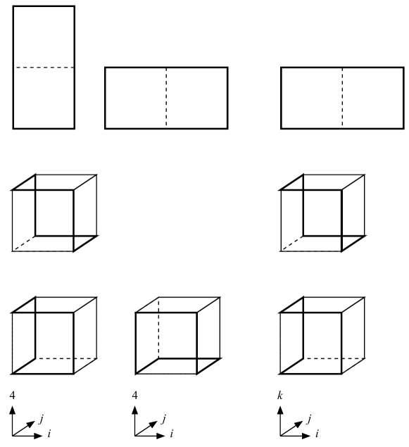
Figure 1: Six-link loops available for improving the gauge action on anisotropic lattices: rectangles (top row); parallelograms (middle); bent rectangles (bottom). Nomenclature from Ref. Luscher:1984xn .

In Appendix C, we show that three of them—all three classes of “bent rectangles” in the bottom row of Fig. 1—may be omitted from an on-shell improved gauge action.

The transformations involving the currents $\bar{q}_{f}\gamma_{\mu}t^{a}q_{f}$ are more interesting. They shift the LE${\cal L}$ [cf. Eq. (2)] by

$${\cal L}_{\mathrm{Sym}}\mapsto{\cal L}_{\mathrm{Sym}} - a^{2}\sum_{f}\varepsilon_{Jf}\bar{q}_{f}\gamma_{4}(\bm{D}\cdot\bm{E}-\bm{E}\cdot\bm{D})q_{f}+a^{2}\sum_{f}(\varepsilon_{Jf}+\delta_{Jf})\bar{q}_{f}[D_{4},\bm{\gamma}\cdot\bm{E}]q_{f}$$ (25)

$$- a^{2}\sum_{f}(\varepsilon_{Jf}+\delta_{Jf})\bar{q}_{f}\bm{\gamma}\cdot(\bm{D}\times\bm{B}+\bm{B}\times\bm{D})q_{f}$$

$$- a^{2}g^{2}\sum_{fg}\varepsilon_{Jf}(\bar{q}_{f}\gamma_{\mu}t^{a}q_{f})(\bar{q}_{g}\gamma_{\mu}t^{a}q_{g})-a^{2}g^{2}\sum_{fg,j}\delta_{Jf}(\bar{q}_{f}\gamma_{j}t^{a}q_{f})(\bar{q}_{g}\gamma_{j}t^{a}q_{g}),\quad\;\quad$$

where the derivatives act only on the gauge fields. The size of these shifts—of order $g^{2}$ for four-quark operators and of order $g^{0}$ for bilinears—is commensurate with the respective terms that already appear in ${\cal L}_{\rm Sym}$. Thus, the $2n_{f}$ parameters $\varepsilon_{Jf}$ and $\delta_{Jf}$ could be used to eliminate bilinears or four-quark operators. For simulations it is preferable to remove the latter, namely $\bar{q}_{f}\gamma_{4}t^{a}q_{f}\bar{q}_{f}\gamma_{4}t^{a}q_{f}$ and $\bar{q}_{f}\bm{\gamma}t^{a}q_{f}\cdot\bar{q}_{f}\bm{\gamma}t^{a}q_{f}$.

We now list the dimension-six four-quark interactions in the LE${\cal L}$. For a single flavor, the complete list is in Table 4, which also indicates that the current-current interactions are redundant.

Table 4: Four-quark interactions that could appear in the LE${\cal L}$ (for a single flavor).

Dim	With axis interchange		Without axis interchange
6	$(\bar{q}t^{a}q)^{2}$		$(\bar{Q}t^{a}Q)^{2}$
	$(\bar{q}\gamma_{5}t^{a}q)^{2}$		$(\bar{Q}\gamma_{5}t^{a}Q)^{2}$
	$(\bar{q}\gamma_{\mu}t^{a}q)^{2}$	$\varepsilon_{J}$	$(\bar{Q}\gamma_{4}t^{a}Q)^{2}$	$\varepsilon_{J}$
			$(\bar{Q}\gamma_{i}t^{a}Q)^{2}$	$\delta_{J}$
	$(\bar{q}\gamma_{\mu}\gamma_{5}t^{a}q)^{2}$		$(\bar{Q}\gamma_{4}\gamma_{5}t^{a}Q)^{2}$
			$(\bar{Q}\gamma_{i}\gamma_{5}t^{a}Q)^{2}$
	$(\bar{q}i\sigma_{\mu\nu}t^{a}q)^{2}$		$(\bar{Q}i\Sigma_{i}t^{a}Q)^{2}$
			$(\bar{Q}\alpha_{i}t^{a}Q)^{2}$

Interactions with the color structure $(\bar{q}\Gamma q)^{2}$ may be omitted, because they can be related to those listed through Fierz rearrangement of the fields.

When considering several flavors of quark, we must keep track of flavor indices as well as color and Dirac indices. The Fierz problem becomes more intricate, and we shall find that color-singlet and color-octet structures should be maintained. Let us start with Fierz rearrangement of the Dirac indices. The four-quark terms in the LE${\cal L}$ take the form

$$\sum_{X}K_{X}\bar{q}_{f\alpha}\Gamma_{X}q_{g\beta}\bar{q}_{h\gamma}\Gamma_{X}q_{i\delta}=-\sum_{X,Y}K_{X}F_{XY}\bar{q}_{f\alpha}\Gamma_{Y}q_{i\delta}\bar{q}_{h\gamma}\Gamma_{Y}q_{g\beta},$$ (26)

where $K_{X}$ denotes short-distance coefficients, the Greek (Latin) indices label color (flavor), $F$ is the Fierz rearrangement matrix (with $F^{2}=1$), and the minus sign comes from anti-commutation of the fermion fields. Equation (26) leaves the flavor and color indices uncontracted, but to get terms in the LE${\cal L}$, the color indices must be contracted (one way or another), and the flavor labels must yield a flavor-neutral interaction. Without loss, we can choose the side of Eq. (26) such that the Dirac matrices contract quark fields of the same flavor. Then one can use Fierz identities for SU($N$) generators (${t^{a}}^{\dagger}=-t^{a}$)

$$Nt^{a}_{\alpha\beta}t^{a}_{\gamma\delta} = -t^{a}_{\alpha\delta}t^{a}_{\gamma\beta}-(N^{2}-1)\delta_{\alpha\delta}\delta_{\gamma\beta}/2N,$$ (27)

$$\delta_{\alpha\beta}\delta_{\gamma\delta} = \delta_{\alpha\delta}\delta_{\gamma\beta}/N-2t^{a}_{\alpha\delta}t^{a}_{\gamma\beta},$$ (28)

so that the color indices are contracted across the same fields as the Dirac and flavor indices.

After using Fierz rearrangement to bring quarks of the same flavor next to each other, one is left with the interactions in Table 5.

Table 5: Four-quark interactions that remain when Fierz rearrangement is taken into account. A sum over Dirac matrices $\Gamma_{X}$ in each of the sets $\{1\}$, $\{\gamma_{4}\}$, $\{\bm{\gamma}\}$, $\{i\bm{\Sigma}\}$, $\{\bm{\alpha}\}$, $\{\bm{\gamma}\gamma_{5}\}$, $\{\gamma_{4}\gamma_{5}\}$, $\{\gamma_{5}\}$ is assumed. (With axis-interchange symmetry, the sets would be $\{1\}$, $\{\gamma_{\mu}\}$, $\{i\sigma_{\mu\nu}\}$, $\{\gamma_{\mu}\gamma_{5}\}$, $\{\gamma_{5}\}$.)

Quarks	Color octet	Color singlet
Heavy-heavy	$\bar{Q}\Gamma_{X}t^{a}Q\,\bar{Q}\Gamma_{X}t^{a}Q$	–
Heavy-heavy	$\bar{Q}_{1}\Gamma_{X}t^{a}Q_{1}\,\bar{Q}_{2}\Gamma_{X}t^{a}Q_{2}$	$\bar{Q}_{1}\Gamma_{X}Q_{1}\,\bar{Q}_{2}\Gamma_{X}Q_{2}$
Heavy-light	$\bar{Q}\Gamma_{X}t^{a}Q\sum_{f}\bar{q}_{f}\Gamma_{X}t^{a}q_{f}$	$\bar{Q}\Gamma_{X}Q\sum_{f}\bar{q}_{f}\Gamma_{X}q_{f}$
Light-light	$\sum_{f}\bar{q}_{f}\Gamma_{X}t^{a}q_{f}\sum_{g}\bar{q}_{g}\Gamma_{X}t^{a}q_{g}$	$\sum_{f}\bar{q}_{f}\Gamma_{X}q_{f}\sum_{g}\bar{q}_{g}\Gamma_{X}q_{g}$

To be concrete, we consider $n_{l}$ flavors of light quarks (with $m_{q}\lesssim\Lambda$) and two flavors of heavy quarks (charm and bottom). We neglect the dependence of the coefficients on the light quark masses, because four-quark interactions are already small corrections (of dimension six). In that case, the four-quark interactions can be arranged so that only the SU($n_{l}$) flavor singlets $\sum_{f}\bar{q}_{f}\Gamma_{X}t^{a}q_{f}$ and $\sum_{f}\bar{q}_{f}\Gamma_{X}q_{f}$ appear.

The parameters $\varepsilon_{Jf}$ and $\delta_{Jf}$ may be used to eliminate color-octet current-current interactions. For each heavy flavor, one finds $(\bar{Q}\gamma_{4}t^{a}Q)^{2}$ and $\sum_{i}(\bar{Q}\gamma_{i}t^{a}Q)^{2}$ to be redundant. For light quarks, we may neglect the differences in the mass, so they have common parameters, and the flavor-singlet combination $(\sum_{f}\bar{q}_{f}\gamma_{\mu}t^{a}q_{f})^{2}$ is redundant. For the light flavors, our list of operators is a Fierz rearrangement of the list in Ref. Sheikholeslami:1985ij .

The leading HQET power counting for heavy-light four-quark operators follows from dimensional analysis and Eq. (17): $\lambda^{2+n_{\Gamma}}$, just as if the light-quark part were replaced by three derivatives. Heavy-heavy four-quark operators will be suppressed, once matrix elements are taken, by a heavy-quark loop, leading to $g^{2}\lambda^{4+n_{\Gamma}}$.

In quarkonium, the size of heavy-light four-quark operators follows similarly from Eq. (18): $\upsilon^{3+n_{\Gamma}}$. The valence heavy-heavy operators are more interesting. They must contain two contributions, one to improve $t$-channel gluon exchange, and another to improve $s$-channel annihilation. The former have NRQCD power counting $g^{2}\upsilon^{3+n_{\Gamma}}\sim\upsilon^{4+n_{\Gamma}}$ (since $g^{2}\sim\upsilon$ Lepage:1992tx ). The latter are $\upsilon^{2}$ times smaller, because the $s$-channel gluon is far off shell, but the Dirac-matrix suppression is now $\upsilon^{1-n_{\Gamma}}$, leading to $g^{2}\upsilon^{6-n_{\Gamma}}\sim\upsilon^{7-n_{\Gamma}}$ in all. In practice, the $s$-channel contributions are suppressed further, when treated as an insertion in a color-singlet quarkonium state. At the tree level, the only color structure that can arise is the color-octet. Its matrix elements vanish in the $\bar{Q}Q$-color-singlet Fock state of quarkonium, leaving the $\upsilon^{3}$-suppressed $\bar{Q}QA$ color octet Bodwin:1994jh . Color-singlet four-quark operators arise at one loop, with an additional factor of $g^{2}\sim\upsilon$.

III New Lattice Action

In this section we introduce a new, improved lattice action for heavy quarks, designed to yield smaller discretization errors than the action in Ref. El-Khadra:1996mp . Our design is based on several lessons from the preceding section and Refs. El-Khadra:1996mp ; Kronfeld:2000ck ; Harada:2001fi . First, it is important to preserve the natural heavy-quark symmetry of Wilson fermions, so that the coefficients $\bar{K}_{i}$ stay bounded for all $m_{Q}a$. (This feature is spoiled in the standard improvement program designed for light quarks, which introduces several new terms that grow with $m_{Q}$.) Second, the new lattice action is flexible enough to match cleanly onto both the Symanzik description and the non-relativistic description.

Let us write the action as follows

$$S=S_{D^{2}F^{2}}+S_{0}+\sum_{d=5}^{\infty}\sum_{n_{\Gamma}=0}^{1}S_{(d,n_{\Gamma})}+S_{\bar{q}q\bar{q}q},$$ (29)

where $S_{D^{2}F^{2}}$ is the improved gauge action [Eq. (172)], $S_{0}$ is the basic Fermilab action, the $S_{(d,n_{\Gamma})}$ consist of the bilinear terms added to improve the quark sector, and $S_{\bar{q}q\bar{q}q}$ denotes four-quark interactions. $S_{(d,n_{\Gamma})}$ consists of (discretizations of) interactions of dimension $d$, with $n_{\Gamma}$ as in the discussion of power counting, Eqs. (16)–(18). Including the interactions in $S_{(d,1)}$ couples “upper” and “lower” components, but allows a smooth limit $a\to 0$. Our aim is to improve the action to include all interactions of dimension six. Then the power counting requires us to include $S_{(7,0)}$ as well. Finally, $S_{\bar{q}q\bar{q}q}$ consists of discretizations of four-quark operators, at dimension six, those of Table 5.

The basic Fermilab action El-Khadra:1996mp is a generalization of the Wilson action Wilson:1975hf :

$$S_{0} = m_{0}a^{4}\sum_{x}\bar{\psi}(x)\psi(x)+a^{4}\sum_{x}\bar{\psi}(x)\gamma_{4}{D_{4}}_{\mathrm{lat}}\psi(x)-{\textstyle\frac{1}{2}}a^{5}\sum_{x}\bar{\psi}(x){\triangle_{4}}_{\mathrm{lat}}\psi(x)$$ (30)

$$+\,\zeta a^{4}\sum_{x}\bar{\psi}(x)\bm{\gamma}\cdot\bm{D}_{\mathrm{lat}}\psi(x)-{\textstyle\frac{1}{2}}r_{s}\zeta a^{5}\sum_{x}\bar{\psi}(x)\triangle^{(3)}_{\mathrm{lat}}\psi(x).$$

We denote lattice fermions fields with $\psi$ to distinguish them from the continuum quark fields in Sec. II. The dimension-five Wilson terms are included in $S_{0}$ to remove doubler states. The remaining dimension-five interactions are Sheikholeslami:1985ij ; El-Khadra:1996mp

$$S_{(5,0)}=S_{B} = -{\textstyle\frac{1}{2}}c_{B}\zeta a^{5}\sum_{x}\bar{\psi}(x)i\bm{\Sigma}\cdot\bm{B}_{\mathrm{lat}}\psi(x),$$ (31)

$$S_{(5,1)}=S_{E} = -{\textstyle\frac{1}{2}}c_{E}\zeta a^{5}\sum_{x}\bar{\psi}(x)\bm{\alpha}\cdot\bm{E}_{\mathrm{lat}}\psi(x),$$ (32)

where the notation $S_{B}$ and $S_{E}$ is from Ref. El-Khadra:1996mp , and the discretizations ${D_{\mu}}_{\mathrm{lat}}$, ${\triangle_{\mu}}_{\mathrm{lat}}$, $\triangle^{(3)}_{\mathrm{lat}}$, $\bm{B}_{\mathrm{lat}}$, $\bm{E}_{\mathrm{lat}}$ are defined below.

The new interactions in Eq. (29) introduced in this paper are

$$S_{(6,0)} = r_{E}a^{6}\sum_{x}\bar{\psi}(x)\{\bm{\gamma}\cdot\bm{D}_{\mathrm{lat}},\bm{\alpha}\cdot\bm{E}_{\mathrm{lat}}\}\psi(x)$$ (33)

$$+ z_{E}a^{6}\sum_{x}\bar{\psi}(x)\gamma_{4}\left(\bm{D}_{\mathrm{lat}}\cdot\bm{E}_{\mathrm{lat}}-\bm{E}_{\mathrm{lat}}\cdot\bm{D}_{\mathrm{lat}}\right)\psi(x),$$

$$S_{(6,1)} = c_{1}a^{6}\sum_{x}\bar{\psi}(x)\sum_{i}\gamma_{i}{D_{i}}_{\mathrm{lat}}{\triangle_{i}}_{\mathrm{lat}}\psi(x)+c_{2}a^{6}\sum_{x}\bar{\psi}(x)\{\bm{\gamma}\cdot\bm{D}_{\mathrm{lat}},\triangle^{(3)}_{\mathrm{lat}}\}\psi(x)$$ (34)

$$+ c_{3}a^{6}\sum_{x}\bar{\psi}(x)\{\bm{\gamma}\cdot\bm{D}_{\mathrm{lat}},i\bm{\Sigma}\cdot\bm{B}_{\mathrm{lat}}\}\psi(x)$$

$$+ z_{3}a^{6}\sum_{x}\bar{\psi}(x)\bm{\gamma}\cdot\left(\bm{D}_{\mathrm{lat}}\times\bm{B}_{\mathrm{lat}}+\bm{B}_{\mathrm{lat}}\times\bm{D}_{\mathrm{lat}}\right)\psi(x)$$

$$+ c_{EE}a^{6}\sum_{x}\bar{\psi}(x)\{\gamma_{4}{D_{4}}_{\mathrm{lat}},\bm{\alpha}\cdot\bm{E}_{\mathrm{lat}}\}\psi(x),$$

$$S_{(7,0)} = c_{4}a^{7}\sum_{x}\bar{\psi}(x)\sum_{i}{\triangle_{i}}_{\mathrm{lat}}^{2}\psi(x)+c_{5}a^{7}\sum_{x}\bar{\psi}(x)\sum_{i}\sum_{j\neq i}\{i\Sigma_{i}{B_{i}}_{\mathrm{lat}},{\triangle_{j}}_{\mathrm{lat}}\}\psi(x)$$ (35)

$$+ r_{5}a^{7}\sum_{x}\bar{\psi}(x)\sum_{i}\sum_{j\neq i}i\Sigma_{i}\left[D_{j}B_{i}D_{j}\right]_{\mathrm{lat}}\psi(x)$$

$$+ z_{6}a^{7}\sum_{x}\bar{\psi}(x)\left(\triangle^{(3)}_{\mathrm{lat}}\right)^{2}\psi(x)+z_{7}a^{7}\sum_{x}\bar{\psi}(x)\{\triangle^{(3)}_{\mathrm{lat}},i\bm{\Sigma}\cdot\bm{B}_{\mathrm{lat}}\}\psi(x)$$

$$+ z^{\prime}_{7}a^{7}\sum_{x}\bar{\psi}(x)[D_{i}i\bm{\Sigma}\cdot\bm{B}D_{i}]_{\mathrm{lat}}\psi(x)$$

$$+ r_{7}a^{7}\sum_{x}\bar{\psi}(x)\bm{\gamma}\cdot\bm{D}_{\mathrm{lat}}i\bm{\Sigma}\cdot\bm{B}_{\mathrm{lat}}\bm{\gamma}\cdot\bm{D}_{\mathrm{lat}}\psi(x)$$

$$+ r^{\prime}_{7}a^{7}\sum_{x}\bar{\psi}(x)[\bm{D}\cdot\left(\bm{B}\times\bm{D}\right)]_{\mathrm{lat}}\psi(x)$$

$$+ r_{BB}a^{7}\sum_{x}\bar{\psi}(x)\left(i\bm{\Sigma}\cdot\bm{B}_{\mathrm{lat}}\right)^{2}\psi(x)+z_{BB}a^{7}\sum_{x}\bar{\psi}(x)\bm{B}_{\mathrm{lat}}\cdot\bm{B}_{\mathrm{lat}}\psi(x)$$

$$- r_{EE}a^{7}\sum_{x}\bar{\psi}(x)\left(\bm{\alpha}\cdot\bm{E}_{\mathrm{lat}}\right)^{2}\psi(x)+z_{EE}a^{7}\sum_{x}\bar{\psi}(x)\bm{E}_{\mathrm{lat}}\cdot\bm{E}_{\mathrm{lat}}\psi(x).$$

All couplings in Eqs. (30)–(35) are real; explicit factors of $i$ are fixed by reflection positivity Osterwalder:1977pc of the continuum action. Some of the improvement terms extend over more than one timeslice, so there are small violations of reflection positivity for the lattice action. We expect that the associated problems are not severe, as with the improved gauge action Luscher:1984is .

Equations (33)–(35) contain 19 new couplings. The convention for couplings $c_{i}$, $r_{i}$ and $z_{i}$ is as follows. In matching calculations we find that couplings $z_{i}$ vanish at the tree level, while the couplings $c_{i}$ do not. Couplings $r_{i}$ are redundant and, for this reason, could be omitted. The analysis in Sect. II gives the number of redundant interactions, rather than the specific choices of interactions themselves. The possibilities for the dimension-7 redundant directions are as follows. One of $(c_{4},c_{5},r_{5})$ is redundant; we choose $r_{5}$. Furthermore, one of $(z_{6},z_{7},r_{7},r_{BB})$, another of $(z_{7},r_{7},r_{BB})$, and another of $(z_{7},r_{7},r^{\prime}_{7},r_{BB})$ are redundant; we choose $r_{7}$, $r^{\prime}_{7}$, and $r_{BB}$. But because pragmatic considerations could motivate other choices, we keep all of them in our analysis. This strategy also provides a good way for the matching calculations to verify the formal analysis of the LE${\cal L}$. In future numerical work, we recommend choosing $r_{s}$, as usual, to solve the doubling problem (in practice $r_{s}\geq 1$). The others may be chosen to save computer time, which presumably means choosing the couplings of computationally demanding interactions to vanish.

The difference operators and fields with the subscript “lat” are taken to be

$${D_{\rho}}_{\mathrm{lat}} = (T_{\rho}-T_{-\rho})/2a$$ (36)

$${\triangle_{\rho}}_{\mathrm{lat}} = (T_{\rho}+T_{-\rho}-2)/a^{2},\quad\triangle^{(3)}_{\mathrm{lat}}=\sum_{i=1}^{3}{\triangle_{i}}_{\mathrm{lat}},$$ (37)

$${F_{\rho\sigma}}_{\mathrm{lat}} = \frac{1}{8a^{2}}\sum_{\bar{\rho}=\pm\rho}\sum_{\bar{\sigma}=\pm\sigma}\mathop{\mathrm{sgn}}\bar{\rho}\mathop{\mathrm{sgn}}\bar{\sigma}\left[T_{\bar{\rho}}T_{\bar{\sigma}}T_{-\bar{\rho}}T_{-\bar{\sigma}}-T_{\bar{\sigma}}T_{\bar{\rho}}T_{-\bar{\sigma}}T_{-\bar{\rho}}\right],$$ (38)

where the covariant translation operators $T_{\pm\rho}$ translate all fields to the right one site in the $\pm\rho$ direction, and multiply by the appropriate link matrix Kronfeld:1984zv . These discretizations are conventional for $S_{0}+S_{B}+S_{E}$. For the new interactions, we have re-used the same ingredients.

For the interactions with couplings $r_{5}$ and $z^{\prime}_{7}$ one can consider

$$\left[D_{j}B_{i}D_{j}\right]_{\mathrm{lat}}={D_{j}}_{\mathrm{lat}}{B_{i}}_{\mathrm{lat}}{D_{j}}_{\mathrm{lat}},$$ (39)

or

$$\left[D_{j}B_{i}D_{j}\right]_{\mathrm{lat}}=\frac{1}{2a^{2}}\left[(1-T_{-j}){B_{i}}_{\mathrm{lat}}(T_{j}-1)+(T_{j}-1){B_{i}}_{\mathrm{lat}}(1-T_{-j})\right].$$ (40)

In tree-level matching calculation, both lead to the same dependence on $r_{5}$ and $z^{\prime}_{7}$. Equation (39) has the advantage that is re-uses elements that are already defined (in a computer program, say) for the dimension-4 and -5 action. Equation (40) is more local, however, and may have other advantages. A FermiQCD DiPierro:2003sz computer code of the new action indicates that Eq. (39) is faster Massimo:2008sz . This code also indicates that it is advantageous to choose the redundant directions so that one may set $r_{5}=r_{7}=0$.

The improved gluon action $S_{D^{2}F^{2}}$ is defined in Appendix C. The four-quark action $S_{\bar{q}q\bar{q}q}$ contains the obvious discretization of the (continuum) operators explained in Sec. II.5 and listed in Tables 4 and 5: simply substitute lattice fermion fields for the continuum fields, and assign each a real coupling. When matching to continuum QCD, the couplings in $S_{\bar{q}q\bar{q}q}$ start at order $g^{2}$, making them commensurate with order-$g^{2}$ matching effects in $S_{(6,1)}+S_{(7,0)}$, such as tree-level quark-quark scattering. To incorporate the four-quark action in a Monte Carlo simulation, one would introduce auxiliary fields to recover a bilinear action. In the next section we show, however, that these operators are not necessary for the target accuracy of 1–2%, so this cumbersome set-up can be avoided for now.

IV Matching Conditions

In this section we derive improvement conditions on the new couplings at the tree level. We calculate on-shell observables for small $\bm{p}a$ without any assumption on $m_{Q}a$. We look at the energy as a function of 3-momentum, which is sensitive to $c_{1}$, $c_{2}$, $c_{4}$, and $z_{6}$. We then look at the interaction of a quark with classical background chromoelectric and chromomagnetic fields. The former is sensitive to $c_{E}$, $r_{E}$, and $z_{E}$; the latter to all but $c_{EE}$, $r_{EE}$, $z_{EE}$, $r_{BB}$, and $z_{BB}$. To ensure that these results are compatible with the improved gauge action, we next compute the amplitude for quark-quark scattering. This step also matches the four-quark interactions, which are not written out explicitly in Sec. III. Finally, we compute the amplitude for Compton scattering to match $c_{EE}$, $r_{EE}$, $z_{EE}$, $r_{BB}$, and $z_{BB}$.

IV.1 Energy

The energy of a heavy quark on the lattice is defined through the exponential fall-off in time of the propagator. For small momentum $\bm{p}$ the energy can be written

$$E=m_{1}+\frac{\bm{p}^{2}}{2m_{2}}-{\textstyle\frac{1}{6}}w_{4}a^{3}\sum_{i}p_{i}^{4}-\frac{\left(\bm{p}^{2}\right)^{2}}{8m_{4}^{3}}+\cdots,$$ (41)

where the coefficients $m_{1}$, $m_{2}$, $m_{4}$ and $w_{4}$ depend on the couplings in the action. Appendix A contains the Feynman rule for the propagator and recalls the general formula for the energy, Eq. (127). By explicit calculation we find

$$m_{1}a = \ln(1+m_{0}a),$$ (42)

$$\frac{1}{m_{2}a} = \frac{2\zeta^{2}}{m_{0}a(2+m_{0}a)}+\frac{r_{s}\zeta}{1+m_{0}a},$$ (43)

$$w_{4} = \frac{2\zeta(\zeta+6c_{1})}{m_{0}a(2+m_{0}a)}+\frac{r_{s}\zeta-24c_{4}}{4(1+m_{0}a)},$$ (44)

$$\frac{1}{m_{4}^{3}a^{3}} = \frac{8\zeta^{4}}{[m_{0}a(2+m_{0}a)]^{3}}+\frac{4\zeta^{4}+8r_{s}\zeta^{3}(1+m_{0}a)}{[m_{0}a(2+m_{0}a)]^{2}}+\frac{r_{s}^{2}\zeta^{2}}{(1+m_{0}a)^{2}}$$ (45)

$$+\frac{32\zeta c_{2}}{m_{0}a(2+m_{0}a)}-\frac{8z_{6}}{1+m_{0}a}.$$

The dimension-6 and -7 couplings $(c_{1},c_{4})$ and $(c_{2},z_{6})$ modify $w_{4}$ and $m_{4}a$, but not $m_{1}a$ or $m_{2}a$.

To match Eq. (41) to the continuum QCD, one requires $m_{4}=m_{2}$ and $w_{4}=0$. From $m_{4}=m_{2}$ one obtains the tuning condition

$$16\zeta c_{2} = \frac{4\zeta^{4}(\zeta^{2}-1)}{[m_{0}a(2+m_{0}a)]^{2}}-\frac{\zeta^{3}[2\zeta+4r_{s}(1+m_{0}a)-6r_{s}\zeta^{2}/(1+m_{0}a)]}{m_{0}a(2+m_{0}a)}$$ (46)

$$+ \frac{3r_{s}^{2}\zeta^{4}}{(1+m_{0}a)^{2}}+\frac{m_{0}a(2+m_{0}a)}{2(1+m_{0}a)}\left[8z_{6}+\frac{r_{s}^{3}\zeta^{3}}{(1+m_{0}a)^{2}}-\frac{r_{s}^{2}\zeta^{2}}{1+m_{0}a}\right],$$

which (at fixed $m_{0}a$) prescribes a line in the $(c_{2},z_{6})$ plane. From $w_{4}=0$ one obtains the tuning condition

$$0=\zeta^{2}+6\zeta c_{1}+\left(r_{s}\zeta-24c_{4}\right)\frac{m_{0}a(2+m_{0}a)}{8(1+m_{0}a)},$$ (47)

which (at fixed $m_{0}a$) prescribes a line in the $(c_{1},c_{4})$ plane. As $m_{0}a\to 0$, both lines become vertical: the coefficients $c_{1}$ and $c_{2}$ of dimension-6 operators are fixed, whereas the coefficients of $c_{4}$ and $z_{6}$ dimension-7 operators are undetermined. At this stage it is tempting to choose $c_{4}$ and $z_{6}$ to be two of the redundant couplings, but below we shall see that there are better choices.

IV.2 Background Field

To compute the interaction of a lattice quark with a continuum background field, we have to compute vertex diagrams with one gluon attached to the quark line. The Feynman rules are given in Eqs. (146) and (147). Our Feynman rules introduce a gauge potential via

$$U_{\mu}(x)=\exp\left[g_{0}A_{\mu}(x+{\textstyle\frac{1}{2}}e_{\mu}a)\right],$$ (48)

where $e_{\mu}$ is a unit vector in the $\mu$ direction, and take the Fourier transform of the gauge field to be

$$A_{\mu}(x)=\int\frac{d^{4}k}{(2\pi)^{4}}e^{ik\cdot x}A_{\mu}(k).$$ (49)

A background field would, however, lead to parallel transporters

$$U_{\mu}(x)={\sf P}\exp\left[g_{0}\int_{0}^{1}A_{\mu}(x+se_{\mu}a)ds\right].$$ (50)

Equation (48) is a convention. If we use Eq. (50) instead, vertices, propagators, and external line factors for gluons would change, in such a way that Feynman diagrams for on-shell amplitudes end up being the same.

To use the interaction with a background classical field as a matching condition, we must compute the current $J_{\mu}$ that couples to the background field $A_{\mu}$ in Eq. (50). Current conservation requires

$$k\cdot J(k)=0,$$ (51)

where $k$ is the external gluon’s momentum. The usual convention for $A_{\mu}(k)$, from Eqs. (48) and (49), yields a current $\hat{J}_{\mu}$ satisfying

$$\hat{k}\cdot\hat{J}(k)=0,$$ (52)

where $\hat{k}_{\mu}=(2/a)\sin(k_{\mu}a/2)$. One sees, therefore, that a classical gluon line with Lorentz index $\mu$ must be multiplied by

$$n_{\mu}(k)=\frac{\hat{k}_{\mu}}{k_{\mu}}\approx 1-\frac{k_{\mu}^{2}a^{2}}{24}.$$ (53)

One should think of $n_{\mu}(k)$ as a wave-function factor for the external line. Its appearance has been noted previously by Weisz Weisz:1982zw .

In the rest of this subsection we match the vertex function in lattice gauge theory with our new action to that in the continuum gauge theory. The incoming quark’s momentum is $p$, the outgoing $p^{\prime}$, and the gluon’s $K=p^{\prime}-p$. The current is given by (no implied sum on $\mu$)

$$J_{\mu}=n_{\mu}(K)\mathcal{N}(p^{\prime})\bar{u}(\xi^{\prime},\bm{p}^{\prime})\Lambda_{\mu}(p^{\prime},p)u(\xi,\bm{p})\mathcal{N}(p),$$ (54)

where $\Lambda_{\mu}(p^{\prime},p)$ is the vertex function derived in Appendix A. The external quarks take normalization factors $\mathcal{N}$ as well as spinor factors El-Khadra:1996mp .

IV.2.1 Chromoelectric field: $\mu=4$

For the interaction with the chromoelectric background field, we use the time component $J_{4}$. To $O(\bm{p}^{2}/m^{2})$ the current in continuum QCD is

$$J_{4}=\bar{u}(\xi^{\prime},\bm{0})\left[1-\frac{\bm{K}^{2}-2i\bm{\Sigma}\cdot(\bm{K}\times\bm{P})}{8m^{2}}\right]u(\xi,\bm{0}),$$ (55)

where $P=(p^{\prime}+p)/2$. After a short calculation with the new lattice action we find

$$J_{4}=\bar{u}(\xi^{\prime},\bm{0})\left[1-\frac{\bm{K}^{2}-2i\bm{\Sigma}\cdot(\bm{K}\times\bm{P})}{8m_{E}^{2}}+\frac{z_{E}\bm{K}^{2}a^{2}}{1+m_{0}a}\right]u(\xi,\bm{0}),$$ (56)

where

$$\frac{1}{4m_{E}^{2}a^{2}}=\frac{\zeta^{2}}{[m_{0}a(2+m_{0}a)]^{2}}+\frac{\zeta^{2}c_{E}}{m_{0}a(2+m_{0}a)}+\frac{2r_{E}}{1+m_{0}a}.$$ (57)

The correct (tree-level) matching is achieved if one adjusts

$$z_{E}=0$$ (58)

and $(c_{E},r_{E})$ such that $m_{E}=m_{2}$:

$$\zeta^{2}c_{E}+r_{E}\frac{2m_{0}a(2+m_{0}a)}{1+m_{0}a}=\frac{\zeta^{2}(\zeta^{2}-1)}{m_{0}a(2+m_{0}a)}+\frac{r_{s}\zeta^{3}}{1+m_{0}a}+\frac{r_{s}^{2}\zeta^{2}m_{0}a(2+m_{0}a)}{4(1+m_{0}a)^{2}}.$$ (59)

At fixed $m_{0}a$ the latter prescribes a line in the $(c_{E},r_{E})$ plane. As before, this line becomes vertical at $m_{0}a=0$, fixing $c_{E}=1$ and leaving $r_{E}$ undetermined.

To obtain conditions on $c_{EE}$, $r_{EE}$, and $z_{EE}$, we shall have to turn to Compton scattering in Sec. IV.4.

IV.2.2 Chromomagnetic field: $\mu=i$

For the interaction with the chromomagnetic background field, we use the spatial components $J_{i}$. To $O(\bm{p}^{3}/m^{3})$ the current in continuum QCD is

$$J_{i} = -i\bar{u}(\xi^{\prime},\bm{0})\left\{P_{i}\left(\frac{1}{m}-\frac{\bm{P}^{2}+{\textstyle\frac{1}{4}}\bm{K}^{2}}{2m^{3}}\right)-\frac{K_{i}\,\bm{P}\cdot\bm{K}}{8m^{3}}\right.$$ (60)

$$\hskip 20.00003pt-\left.\varepsilon_{ijl}i\Sigma_{l}K_{j}\left(\frac{1}{2m}-\frac{\bm{P}^{2}+{\textstyle\frac{1}{4}}\bm{K}^{2}}{4m^{3}}\right)+\varepsilon_{ijl}i\Sigma_{l}P_{j}\frac{\bm{P}\cdot\bm{K}}{4m^{3}}\right\}u(\xi,\bm{0}).$$

After another short calculation we find

$$J_{i} = -i\bar{u}(\xi^{\prime},\bm{0})\left\{P_{i}\left(\frac{1}{m_{2}}-\frac{\bm{P}^{2}+{\textstyle\frac{1}{4}}\bm{K}^{2}}{2m_{4}^{3}}\right)-\frac{K_{i}\,\bm{P}\cdot\bm{K}}{8m_{2}m_{E}^{2}}+\frac{z_{E}a^{2}K_{i}\,\bm{P}\cdot\bm{K}}{m_{2}(1+m_{0}a)}\right.$$ (61)

$$\hskip 20.00003pt+\left.{\textstyle\frac{1}{8}}w_{B_{1}}a^{3}\left[P_{i}\bm{K}^{2}-K_{i}\,\bm{P}\cdot\bm{K}\right]-{\textstyle\frac{1}{16}}w_{B_{2}}a^{3}\varepsilon_{ijl}K_{j}i\Sigma_{l}\bm{K}^{2}\right.$$

$$\hskip 20.00003pt-\left.{\textstyle\frac{1}{4}}w_{B_{3}}a^{3}\varepsilon_{ijl}K_{j}P_{l}i\bm{\Sigma}\cdot\bm{P}+{\textstyle\frac{1}{4}}w_{X}a^{3}X_{i}\right.$$

$$\hskip 20.00003pt-\left.{\textstyle\frac{2}{3}}w_{4}a^{3}P_{i}(P_{i}^{2}+{\textstyle\frac{1}{4}}K_{i}^{2})+{\textstyle\frac{1}{12}}w^{\prime}_{B}a^{3}\varepsilon_{ijl}i\Sigma_{l}K_{j}(K_{i}^{2}+K_{j}^{2})\right.$$

$$\hskip 20.00003pt+\left.{\textstyle\frac{1}{12}}(w_{4}+w_{4}^{\prime})a^{3}\varepsilon_{ijl}i\Sigma_{l}K_{j}[(3P_{i}^{2}+{\textstyle\frac{1}{4}}K_{i}^{2})+(3P_{j}^{2}+{\textstyle\frac{1}{4}}K_{j}^{2})]\right.$$

$$\hskip 20.00003pt-\left.\varepsilon_{ijl}i\Sigma_{l}K_{j}\left(\frac{1}{2m_{B}}-\frac{\bm{P}^{2}+{\textstyle\frac{1}{4}}\bm{K}^{2}}{4m_{B^{\prime}}^{3}}\right)+\varepsilon_{ijl}i\Sigma_{l}P_{j}\frac{\bm{P}\cdot\bm{K}}{4m_{2}m_{E}^{2}}\right\}u(\xi,\bm{0}),$$

where $m_{2}$, $m_{4}^{3}$, $w_{4}$, and $m_{E}^{2}$ have been introduced already, and

$$\frac{1}{m_{B}a} = \frac{1}{m_{2}a}+\frac{(c_{B}-r_{s})\zeta}{1+m_{0}a},$$ (62)

$$\frac{1}{m_{B^{\prime}}^{3}a^{3}} = \frac{1}{m_{4}^{3}a^{3}}-\frac{r_{s}(r_{s}-c_{B})\zeta^{2}}{(1+m_{0}a)^{2}}+\frac{8(z_{6}-z_{7})+4(r_{7}-z^{\prime}_{7})}{1+m_{0}a},$$ (63)

$$w_{B_{3}} = \frac{4(r_{s}-c_{B})\zeta^{3}(1+m_{0}a)}{[m_{0}a(2+m_{0}a)]^{2}}+\frac{16(c_{2}-c_{3})\zeta}{m_{0}a(2+m_{0}a)}+\frac{8r_{7}}{1+m_{0}a},$$ (64)

$$w_{B_{2}} = w_{B_{3}}+\frac{16z_{3}\zeta}{m_{0}a(2+m_{0}a)}-\frac{8z^{\prime}_{7}}{1+m_{0}a},$$ (65)

$$w_{B_{1}} = w_{B_{2}}-\frac{8(r^{\prime}_{7}-z^{\prime}_{7})}{1+m_{0}a},$$ (66)

$$w^{\prime}_{B} = \frac{c_{B}\zeta-4(c_{5}-r_{5})}{1+m_{0}a},$$ (67)

$$w^{\prime}_{4} = -\frac{r_{s}\zeta-24c_{4}+16(2c_{5}+r_{5})}{4(1+m_{0}a)}.$$ (68)

The term $w_{X}a^{3}\bm{X}$ is discussed below.

Comparing Eqs. (60) and (61), one sees that the first four terms match the continuum if $m_{2}=m_{4}=m_{E}=m$. The other terms do not match unless one adjusts $c_{B}=r_{s}$ El-Khadra:1996mp and $z_{E}=0$ [as in Eq. (58)] and, furthermore, demands $w_{4}=w^{\prime}_{4}=w_{B_{1}}=w_{B_{2}}=w_{B_{3}}=w^{\prime}_{B}=0$:

$$c_{3} = c_{2}+\frac{r_{7}}{\zeta}\frac{m_{0}a(2+m_{0}a)}{2(1+m_{0}a)},$$ (69)

$$z_{3} = \frac{r^{\prime}_{7}}{\zeta}\frac{m_{0}a(2+m_{0}a)}{2(1+m_{0}a)},$$ (70)

$$c_{4} = {\textstyle\frac{1}{24}}r_{s}\zeta+{\textstyle\frac{1}{3}}c_{B}\zeta+2r_{5},$$ (71)

$$c_{5} = {\textstyle\frac{1}{4}}c_{B}\zeta+r_{5},$$ (72)

$$z_{7} = z_{6}+{\textstyle\frac{1}{2}}(r_{7}-r^{\prime}_{7}),$$ (73)

$$z^{\prime}_{7} = r^{\prime}_{7}.$$ (74)

Taken with Eqs. (46) and (47), these tuning conditions put eight constraints on the nine (non-redundant) couplings for interactions made solely out of spatial derivatives (and, hence, chromomagnetic fields). To eliminate $z_{6}$ from the right-hand side of Eq. (73), and to obtain conditions on $r_{BB}$ and $z_{BB}$, we shall have to turn to Compton scattering in Sec. IV.4.

Equations (69)–(74) make concrete several abstract features of Sec. II. If one would like to take $c_{4}$ to be redundant in Eq. (47), then one cannot take $r_{5}$ to be redundant here, and similarly for $z_{6}$ and $r_{7}$ or $r^{\prime}_{7}$. Also, a mistuned $c_{5}-r_{5}$ leads to $w^{\prime}_{B}\neq 0$ and a spin-dependent contribution $[1+{\textstyle\frac{1}{6}}w^{\prime}_{B}m_{2}a(K_{i}^{2}+K_{j}^{2})a^{2}]\varepsilon_{ijl}i\Sigma_{l}K_{j}/2m_{2}$. The mismatch here is suppressed by $\lambda^{2}$ in the HQET counting—as expected from Table 2—and by $a^{3}$ in the usual Symanzik counting.

The only undesired term in Eq. (61) not yet discussed is ${\textstyle\frac{1}{4}}w_{X}a^{3}X_{i}$, where

$$\bm{X} = (i\bm{\Sigma}\times\bm{K})\,\bm{P}^{2}-(i\bm{\Sigma}\times\bm{P})\,\bm{P}\cdot\bm{K}-\bm{P}\,[i\bm{\Sigma}\cdot(\bm{K}\times\bm{P})]+(\bm{K}\times\bm{P})\,i\bm{\Sigma}\cdot\bm{P},\quad$$ (75)

$$w_{X} = \frac{4r_{s}\zeta^{3}(1+m_{0}a)}{[m_{0}a(2+m_{0}a)]^{2}}+\frac{16c_{2}\zeta}{m_{0}a(2+m_{0}a)}.$$ (76)

One cannot tune $w_{X}=0$. Fortunately, however, $\bm{X}=\bm{0}$. A simple geometric proof is as follows: if, by chance, $\bm{P}$ is parallel to $\bm{K}$, then setting $\bm{P}\propto\bm{K}$ one sees that the last two terms on the right-hand side of Eq. (75) vanish and the first two cancel. In the general case that $\bm{P}$ is not parallel to $\bm{K}$, then $\bm{K}$, $\bm{P}$, and $\bm{K}\times\bm{P}$ are three linearly independent vectors. But one easily sees that

$$\bm{K}\cdot\bm{X}=\bm{P}\cdot\bm{X}=(\bm{K}\times\bm{P})\cdot\bm{X}=0;$$ (77)

thus, $\bm{X}=\bm{0}$. Such identities are very useful in simplifying expressions for the Compton scattering amplitude.

IV.3 Quark-quark scattering

To match the four-quark action, $S_{\bar{q}q\bar{q}q}$, one must work out the quark-quark scattering amplitude. With the current $J_{\mu}$ derived in the previous subsection, this is a relatively simple task. The main new ingredient is the improved gluon propagator. For $k^{2}a^{2}\ll 1$, one finds Weisz:1982zw

$$D_{\mu\nu}(k)=n_{\mu}(k)D_{\mu\nu}^{\rm cont}(k)n_{\nu}(k)\left[1+xa^{2}k^{2}\right]+O(a^{4}),$$ (78)

where $x$ is the redundant coupling of the pure-gauge action, cf. Appendix C and Ref. Luscher:1984xn . This approximation suffices for evaluating $t$-channel gluon exchange. Once the bilinear action has been matched correctly, the lattice amplitude (using, say, Feynman gauge) is clearly merely

$$\mathcal{A}_{\rm lat}(12\to 12)=\mathcal{A}_{\rm cont}(12\to 12)+xa^{2}t^{a}J_{1}\cdot J_{2}t^{a},$$ (79)

where 1 and 2 label the scattered quark flavors, and both $t^{a}$ have uncontracted color indices. We find, therefore, that the tree-level couplings of $S_{\bar{q}q\bar{q}q}$ are, at most, proportional to $x$. They can be eliminated, at the tree level, by setting $x=0$, with the added benefit of simplifying the gauge action $S_{D^{2}F^{2}}$.

Note, however, that the approximation in Eq. (78) and, thus, Eq. (79), breaks down for $s$-channel annihilation of heavy quarks. As discussed in Sec. II.5, these interactions are suppressed for other reasons, so the four-quark operators needed to correct them may be neglected.

IV.4 Compton scattering

The matching of Secs. IV.1–IV.3 leaves four non-redundant couplings of the new action undetermined: $z_{6}$, $c_{EE}$, $z_{EE}$, and $z_{BB}$. To find four more matching conditions, we turn to Compton scattering. We shall proceed with the gauge-action redundant coupling $x=0$.

The amplitude is

$$\mathcal{A}_{\rm lat}^{ab}(qg\to qg)=\sum_{\mu\nu}\bar{\epsilon}^{\prime}_{\nu}(k^{\prime})n_{\nu}(k^{\prime})\hat{\mathcal{M}}_{\mu\nu}^{ab}\epsilon_{\mu}(k)n_{\mu}(k),$$ (80)

where $\bar{\epsilon}_{\nu}$ and $\epsilon_{\mu}$ are continuum polarization vectors, and $\hat{\mathcal{M}}_{\mu\nu}^{ab}$ denotes the sum of Feynman diagrams shown in Fig. 2.

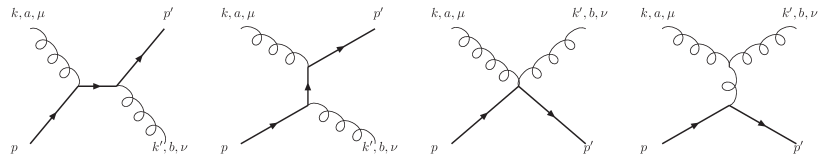
Figure 2: Feynman diagrams for Compton scattering in lattice gauge theory.

The factors $n_{\nu}(k^{\prime})$ and $n_{\mu}(k)$ appear in Eq. (80) to account for lattice gluons. With them one can verify that

$$\sum_{\rm pol.}\epsilon_{\mu}(k)n_{\mu}(k)n_{\nu}(k)\bar{\epsilon}_{\nu}(k)=-D_{\mu\nu}(k),$$ (81)

as usual. We find it convenient to associate these factors with the diagrams and introduce $\mathcal{M}_{\mu\nu}^{ab}=n_{\nu}(k^{\prime})\hat{\mathcal{M}}_{\mu\nu}^{ab}n_{\mu}(k)$. Then

$$\mathcal{M}_{\mu\nu}^{ab} = t^{b}t^{a}n_{\nu}(k^{\prime})\mathcal{N}(p^{\prime})\bar{u}(\xi^{\prime},\bm{p}^{\prime})\Lambda_{\nu}(p^{\prime},q)S(q)\Lambda_{\mu}(q,p)u(\xi,\bm{p})\mathcal{N}(p)n_{\mu}(k)$$

$$+ t^{a}t^{b}n_{\nu}(k^{\prime})\mathcal{N}(p^{\prime})\bar{u}(\xi^{\prime},\bm{p}^{\prime})\Lambda_{\mu}(p^{\prime},q^{\prime})S(q^{\prime})\Lambda_{\mu}(q^{\prime},p)u(\xi,\bm{p})\mathcal{N}(p)n_{\mu}(k)$$

$$- {\textstyle\frac{1}{2}}\{t^{a},t^{b}\}n_{\nu}(k^{\prime})\mathcal{N}(p^{\prime})\bar{u}(\xi^{\prime},\bm{p}^{\prime})aX_{\mu\nu}(p,k,-k^{\prime})u(\xi,\bm{p})\mathcal{N}(p)n_{\mu}(k)$$

$$- {\textstyle\frac{1}{2}}[t^{a},t^{b}]n_{\nu}(k^{\prime})\mathcal{N}(p^{\prime})\bar{u}(\xi^{\prime},\bm{p}^{\prime})aY_{\mu\nu}(p,k,-k^{\prime})u(\xi,\bm{p})\mathcal{N}(p)n_{\mu}(k),$$

$$+ t^{c}V^{abc}_{\mu\nu\sigma}(k,-k^{\prime},-K)D_{\sigma\rho}(K)n_{\nu}(k^{\prime})\mathcal{N}(p^{\prime})\bar{u}(\xi^{\prime},\bm{p}^{\prime})\Lambda_{\rho}(p^{\prime},p)u(\xi,\bm{p})\mathcal{N}(p)n_{\mu}(k)$$

where $q=p+k=p^{\prime}+k^{\prime}$, $q^{\prime}=p-k^{\prime}=p^{\prime}-k$, $K=k-k^{\prime}=p^{\prime}-p$. The propagator $S(q)$ and vertex factors $\Lambda_{\mu}$, $X_{\mu\nu}$ and $Y_{\mu\nu}$ are defined in Appendix A. The gluon propagator, to the accuracy needed, is given in Eq. (78), and to the same accuracy the triple-gluon vertex is (with $x=0$)

$$V^{abc}_{\mu\nu\sigma}(k,-k^{\prime},-K) = if^{abc}\left[n_{\mu}(k)n_{\nu}(k^{\prime})n_{\sigma}(K)\right]^{-1}\left\{\vphantom{{\textstyle\frac{1}{2}}}\right.$$ (83)

$$\delta_{\mu\nu}[(k+k^{\prime})_{\sigma}(1-{\textstyle\frac{1}{12}}\delta_{\mu\sigma}K^{2}a^{2})+{\textstyle\frac{1}{12}}K_{\sigma}(k^{2}_{\mu}-{k^{\prime}_{\mu}}^{2})a^{2}]$$

$$- \delta_{\nu\sigma}[(k^{\prime}-K)_{\mu}(1-{\textstyle\frac{1}{12}}\delta_{\nu\mu}k^{2}a^{2})+{\textstyle\frac{1}{12}}k_{\mu}({k^{\prime}_{\nu}}^{2}-K_{\nu}^{2})a^{2}]$$

$$- \delta_{\sigma\mu}[(K+k)_{\nu}(1-{\textstyle\frac{1}{12}}\delta_{\sigma\nu}{k^{\prime}}^{2}a^{2})-{\textstyle\frac{1}{12}}k^{\prime}_{\nu}(K^{2}_{\sigma}-k_{\sigma}^{2})a^{2}]\left.\vphantom{{\textstyle\frac{1}{2}}}\right\}.$$

Note that the factors $n_{\sigma}(K)$, etc., arise naturally. Note also that $K\cdot J=k\cdot\epsilon=k^{\prime}\cdot\bar{\epsilon}^{\prime}=k^{2}={k^{\prime}}^{2}=0$, so most of the lattice artifacts in the vertex drop out. The remaining one is necessary to cancel a similar lattice artifact from the other diagrams, cf. Eqs. (164) and (165).

We may choose the polarization vectors such that $\bar{\epsilon}^{\prime}_{4}=\epsilon_{4}=0$. Then we need only focus on $\mathcal{M}_{mn}$. We have verified that $\mathcal{M}_{44}$ is improved by (a subset of) the improvement conditions needed for $\mathcal{A}(qg\to qg)$ calculated with these polarization vectors.

The present the results, let us introduce some notation. Write the momenta as

$$P = (p^{\prime}+p)/2,$$ (84)

$$R = (k+k^{\prime})/2,$$ (85)

$$K = p^{\prime}-p=k-k^{\prime},$$ (86)

so $q=P+R$ and $q^{\prime}=P-R$. Note that $P_{0}=-iP_{4}=2m_{1}+\cdots$ is larger than the other momenta, and $K_{0}=-iK_{4}=({\bm{p}^{\prime}}^{2}-\bm{p}^{2})/2m_{2}$ is smaller. Next separate the diagrams according to a color decomposition,

$$\mathcal{M}_{\mu\nu}^{ab}={\textstyle\frac{1}{2}}\{t^{a},t^{b}\}\mathcal{M}_{\mu\nu}+{\textstyle\frac{1}{2}}[t^{a},t^{b}]\mathcal{N}_{\mu\nu},$$ (87)

where the second term would be absent in an Abelian gauge theory. Finally, write

$$\mathcal{M}_{\mu\nu}=\sum_{n=0}^{3}\sum_{s=0}^{n}R_{0}^{n-1-2s}\mathcal{M}_{\mu\nu}^{(n,n-1-2s)},$$ (88)

and similarly for $\mathcal{N}_{\mu\nu}$, where the superscript $(n,r)$ denotes the power in $1/m$ and $R_{0}$.

Most of these terms are well-matched with Eqs. (58), (59), (69)–(74). New matching conditions come from $\mathcal{M}_{mn}^{(3,2)}$, $\mathcal{N}_{mn}^{(3,2)}$, $\mathcal{M}_{mn}^{(3,0)}$, and $\mathcal{N}_{mn}^{(3,0)}$. The $(n,r)=(3,2)$ amplitudes are

$$\mathcal{M}_{mn}^{(3,2)} = \frac{\delta_{mn}}{4m_{EE}^{3}}+\frac{2a^{3}z_{EE}\delta_{mn}}{1+m_{0}a},$$ (89)

$$\mathcal{N}_{mn}^{(3,2)} = \frac{\varepsilon_{mni}i\Sigma_{i}}{4m_{EE}^{3}},$$ (90)

where

$$\frac{1}{m_{EE}^{3}a^{3}} = \frac{8[\zeta+{\textstyle\frac{1}{2}}c_{E}\zeta m_{0}a(2+m_{0}a)]^{2}}{[m_{0}a(2+m_{0}a)]^{3}}+\frac{4\zeta^{2}}{[m_{0}a(2+m_{0}a)]^{2}}$$ (91)

$$+ \frac{16c_{EE}\zeta}{m_{0}a(2+m_{0}a)(1+m_{0}a)}+\frac{8(c_{EE}\zeta+r_{EE})}{1+m_{0}a}.$$

To match to continuum QCD one requires

$$z_{EE}=0$$ (92)

and the adjustment of $(c_{EE},r_{EE})$ so that $m_{EE}=m_{2}$. As with, say, $(c_{E},r_{E})$, at fixed $m_{0}a$ the latter prescribes a line in the $(c_{EE},r_{EE})$ plane, which becomes vertical at $m_{0}a=0$, fixing $c_{EE}=-{\textstyle\frac{1}{8}}$ and leaving $r_{EE}$ undetermined.

The $(n,r)=(3,0)$ amplitudes are

$$\mathcal{M}_{mn}^{(3,0)} = \left.\mathcal{M}_{mn}^{(3,0)}\right|_{\rm matched}-\frac{2a^{3}}{e^{m_{1}a}}(z_{BB}+z_{6}+r_{7}-r_{BB}-z^{\prime}_{7})M_{mn},$$ (93)

$$M_{mn} = \delta_{mn}(\bm{R}^{2}-{\textstyle\frac{1}{4}}\bm{K}^{2})-(R_{m}-{\textstyle\frac{1}{2}}K_{m})(R_{n}+{\textstyle\frac{1}{2}}K_{n}),$$ (94)

$$\mathcal{N}_{mn}^{(3,0)} = \left.\mathcal{N}_{mn}^{(3,0)}\right|_{\rm matched}-\frac{2a^{3}}{e^{m_{1}a}}(z_{6}+r_{7}-r_{BB}-z^{\prime}_{7})N_{mn},$$ (95)

$$N_{mn} = \varepsilon_{mnr}(R_{r}i\bm{\Sigma}\cdot\bm{R}-{\textstyle\frac{1}{4}}K_{r}i\bm{\Sigma}\cdot\bm{K})-{\textstyle\frac{1}{2}}(i\Sigma_{n}\varepsilon_{mrs}+i\Sigma_{m}\varepsilon_{nrs})R_{r}K_{s},$$ (96)

where “matched” denotes terms (spelled out in Appendix B) that already match, if the conditions derived so far are applied. Equations (93) and (95) yield the new conditions

$$z_{BB}+z_{6}-z^{\prime}_{7} = r_{BB}-r_{7},$$ (97)

$$z_{6}-z^{\prime}_{7} = r_{BB}-r_{7}.$$ (98)

Solving these, and noting $z^{\prime}_{7}=r^{\prime}_{7}$ [Eq. (74)], we find

$$z_{BB} = 0,$$ (99)

$$z_{6} = r_{BB}+r^{\prime}_{7}-r_{7},$$ (100)

which completes the set of conditions needed to match the new lattice action.

IV.5 Matching Summary

Equations (46), (47), (71)–(74), (99), and (100) can now be combined to yield

$$6\zeta c_{1} = -\zeta^{2}+(c_{B}\zeta+6r_{5})\frac{m_{0}a(2+m_{0}a)}{1+m_{0}a},$$ (101)

$$16\zeta c_{2} = \frac{4\zeta^{4}(\zeta^{2}-1)}{[m_{0}a(2+m_{0}a)]^{2}}-\frac{\zeta^{3}[2\zeta+4r_{s}(1+m_{0}a)-6r_{s}\zeta^{2}/(1+m_{0}a)]}{m_{0}a(2+m_{0}a)}$$

$$+ \frac{3r_{s}^{2}\zeta^{4}}{(1+m_{0}a)^{2}}+\frac{m_{0}a(2+m_{0}a)}{2(1+m_{0}a)}\left[8(r_{BB}+r^{\prime}_{7}-r_{7})+\frac{r_{s}^{3}\zeta^{3}}{(1+m_{0}a)^{2}}-\frac{r_{s}^{2}\zeta^{2}}{1+m_{0}a}\right],$$

$$c_{3} = c_{2}+\frac{r_{7}}{\zeta}\frac{m_{0}a(2+m_{0}a)}{2(1+m_{0}a)}+\frac{(r_{s}-c_{B})\zeta^{2}(1+m_{0}a)}{4m_{0}a(2+m_{0}a)},$$ (103)

$$c_{4} = {\textstyle\frac{1}{24}}r_{s}\zeta+{\textstyle\frac{1}{3}}c_{B}\zeta+2r_{5},$$ (104)

$$c_{5} = {\textstyle\frac{1}{4}}c_{B}\zeta+r_{5},$$ (105)

$$z_{3} = \frac{r^{\prime}_{7}}{\zeta}\frac{m_{0}a(2+m_{0}a)}{2(1+m_{0}a)},$$ (106)

$$z_{6} = r_{BB}+r^{\prime}_{7}-r_{7},$$ (107)

$$z_{7} = r_{BB}-{\textstyle\frac{1}{2}}(r_{7}-r^{\prime}_{7}),$$ (108)

$$z^{\prime}_{7} = r^{\prime}_{7},$$ (109)

$$z_{BB} = 0,$$ (110)

To run a numerical simulation, we would like to have as few new couplings as possible. The matching calculations verified the presence of several redundant directions. We may, therefore, take

$$r_{5}=r_{7}=r^{\prime}_{7}=r_{BB}=0$$ (111)

to all orders in perturbation theory. Hence

$$c_{B} = r_{s},$$ (112)

$$c_{1} = -{\textstyle\frac{1}{6}}\zeta+c_{B}\frac{m_{0}a(2+m_{0}a)}{6(1+m_{0}a)},$$ (113)

$$c_{2}=c_{3} = \frac{\zeta^{3}(\zeta^{2}-1)}{[2m_{0}a(2+m_{0}a)]^{2}}-\frac{\zeta^{2}[\zeta+2r_{s}(1+m_{0}a)-3r_{s}\zeta^{2}/(1+m_{0}a)]}{8m_{0}a(2+m_{0}a)}$$ (114)

$$+ \frac{3r_{s}^{2}\zeta^{3}}{16(1+m_{0}a)^{2}}+\frac{m_{0}a(2+m_{0}a)r_{s}^{2}\zeta}{32(1+m_{0}a)^{2}}\left[\frac{r_{s}\zeta}{1+m_{0}a}-1\right],$$

$$c_{4} = {\textstyle\frac{1}{24}}r_{s}\zeta+{\textstyle\frac{1}{3}}c_{B}\zeta,$$ (115)

$$c_{5} = {\textstyle\frac{1}{4}}c_{B}\zeta,$$ (116)

and

$$z_{3}=z_{6}=z_{7}=z^{\prime}_{7}=z_{BB}=0.$$ (117)

From the chromoelectric interactions we require $m_{E}=m_{2}$ and $m_{EE}=m_{2}$, whence

$$c_{E}=\frac{\zeta^{2}-1}{m_{0}a(2+m_{0}a)}+\frac{r_{s}\zeta}{1+m_{0}a}+\frac{r_{s}^{2}m_{0}a(2+m_{0}a)}{4(1+m_{0}a)^{2}}-\frac{r_{E}}{\zeta^{2}}\frac{2m_{0}a(2+m_{0}a)}{1+m_{0}a},$$ (118)

$$c_{EE}[2+m_{0}a(2+m_{0}a)] = \frac{\zeta(\zeta^{2}-1)(1+m_{0}a)}{[m_{0}a(2+m_{0}a)]^{2}}+\frac{c_{E}\zeta(\zeta^{2}-1)(1+m_{0}a)}{m_{0}a(2+m_{0}a)}$$ (119)

$$+ \frac{\zeta(r_{s}\zeta-1-m_{0}a)}{2m_{0}a(2+m_{0}a)}+{\textstyle\frac{1}{2}}r_{s}c_{E}\zeta^{2}+2r_{E}\zeta-{\textstyle\frac{1}{4}}c_{E}^{2}\zeta(1+m_{0}a)$$

$$+ \frac{r_{s}r_{E}m_{0}a(2+m_{0}a)}{1+m_{0}a}-\frac{r_{EE}}{\zeta}m_{0}a(2+m_{0}a),$$

and we also find

$$z_{E}=z_{EE}=0.$$ (120)

Without loss one may set the redundant $r_{E}=r_{EE}=0$ to simplify the action and Eqs. (118) and (119).

In summary, of the nineteen new couplings in Eqs. (33)–(35), we find only six that are non-zero at tree-level matching. Moreover, once the bilinear action has been matched, and the redundant gauge coupling $x=0$, the only non-zero four-quark interaction would correspond to (highly suppressed) $Q\bar{Q}$ annihilation. In the next section we shall examine the size of the remaining uncertainties, to justify that this level of matching suffices.

V Errors from Truncation

In this section we give a semi-quantitative analysis of heavy-quark discretization effects with the new action. Our aim is to study the accuracy needed in matching lattice gauge theory to continuum QCD. Several elements are needed. First, we need estimates of the mismatch at short distances. This is straightforward, because the calculations of Sec. IV can be applied to work out how large the mismatch is for the unimproved action. Second, we need estimates of the long-distance effects, which is possible parametrically, by counting powers of $\Lambda$ and $\upsilon$. Finally, the size of discretization effects depends on the lattice spacing (obviously) so we must note the range that is tractable today and in the near future.

The error analysis is convenient using the non-relativistic description. Heavy-quark effects of operators that are related as in Eqs. (14) and (15) are lumped into one short-distance coefficient ${\cal C}_{i}^{\mathrm{lat}}$ per HQET operator in Table 3. In Sec. IV the short-distance coefficients are $1/2m_{2}$, $1/2m_{B}$, $1/4m_{E}^{2}$, $1/8m_{4}^{3}$, $w_{4}$, $w_{B_{i}}$, etc. In the corresponding continuum short-distance coefficients ${\cal C}_{i}^{\mathrm{cont}}$, these masses are replaced with a single mass $m_{Q}$. To eliminate discretization effects from the kinetic energy, one should identify $m_{Q}$ with $m_{2}$.

Comparison of Eqs. (5) and (6) then says that heavy-quark discretization effects take the form

$$\mathtt{error}_{i}=\left({\cal C}_{i}^{\mathrm{lat}}-{\cal C}_{i}^{\mathrm{cont}}\right)\langle{\cal O}_{i}\rangle.$$ (121)

For example, the error from $(\bm{p}^{2})^{2}/8m_{4}^{3}$ is

$$\mathtt{error}_{m_{4}}=\left(\frac{1}{8m_{4}^{3}a^{3}}-\frac{1}{(2m_{2}a)^{3}}\right)a^{3}\langle(\bm{p}^{2})^{2}\rangle.$$ (122)

See Refs. Kronfeld:2000ck ; Harada:2001fi for further details, and Ref. Kronfeld:2003sd for the application of this technique to compare several heavy-quark formalisms. We estimate the matrix elements $\langle{\cal O}_{i}\rangle$ using the power counting of HQET and NRQCD for heavy-light hadrons and quarkonium, respectively. The power of $\lambda$ or $\upsilon$ is listed in Table 3. The coefficient mismatches are obtained from Sec. IV, where explicit expressions show how the coefficients depend on the new couplings. In particular, when the new couplings vanish, we derive the mismatch for the Wilson and clover actions.

Explicit calculations of the mismatch at higher orders of perturbation theory are not yet available. (They would be tantamount to higher-loop matching.) Nevertheless, the asymptotic behavior remains constrained, when $m_{Q}a\ll 1$ because of the presence of the $\mathcal{E}$-type operators, when $m_{Q}a\not\ll 1$ by heavy-quark symmetry, and when $m_{Q}a\sim 1$ because the Wilson time derivative ensures only one pole in the propagator Kronfeld:2000ck . It turns out that the most pessimistic asymptotic behavior for $1/2m_{B}$, $1/4m_{E}^{2}$, etc., is the same at higher orders as in the tree level formulas in Sec. IV. It seems reasonable, therefore, to multiply the tree-level mismatch with $\alpha_{s}^{l}$ to estimate the $l$-loop mismatch. We use one-loop running for $\alpha_{s}(a)$ starting with $\alpha_{s}(1/11~{}{\rm fm})=1/3$. This yields the high end of the Brodsky-Lepage-Mackenzie coupling Brodsky:1982gc calculated for similar quantities Harada:2002jh .

The resulting estimates for the mismatch of rotationally symmetric operators are shown in Fig. 3, as a function of the lattice spacing $a=m_{2}a/m_{Q}$, $Q\in\{c,b\}$.

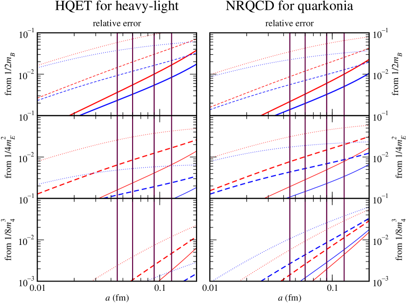
Figure 3: Relative truncation errors for the new action. The light gray or red curves stand for $c$ quarks; dark gray or blue for $b$. Dotted curves show the error when the contribution is unimproved. Dashed and solid curves show the error for tree-level and one-loop matching, respectively, of the needed operators. $\Lambda=700$ MeV, $m_{c}=1400$ MeV, $m_{b}=4200$ MeV; $\upsilon^{2}_{\bar{c}c}=0.3$, $\upsilon^{2}_{\bar{b}b}=0.1$. Vertical lines show lattice spacings available with the MILC ensembles Bernard:2001av .

We show the relative error in mass splittings, which are of order $\Lambda$ in heavy-light hadrons and of order $m_{Q}\upsilon^{2}$ in quarkonium. The left set of plots uses HQET power counting, for heavy-light hadrons, while the right set of plots uses NRQCD power counting, for quarkonia. The light gray or red (dark gray or blue) curves show the estimate for hadrons containing $c$ ($b$) quarks. The dotted curves show the error when the corresponding correction term is omitted completely, i.e., the errors in the Wilson action. The dashed (solid) curves show the estimate of the error for tree-level (one-loop) matching. The vertical lines highlight $a=0.125$ fm, $0.09$ fm, $0.06$ fm and $0.045$ fm, corresponding to the ensembles of gauge fields with $n_{f}=2+1$ flavors from the MILC collaboration Bernard:2001av .

To drive the each contribution to heavy-quark discretization effects below 1%, we find that one-loop matching is necessary for $c_{B}$, the coupling of the chromomagnetic clover term. Tree-level matching is sufficient for the chromoelectric clover coupling $c_{E}$, though one-loop matching would be desirable for charmonium and charmed hadrons. The lowest plots, labeled “from $1/8m_{4}^{3}$” are for the relativistic correction terms, with couplings $c_{2}$ and $z_{6}$. They also apply to $1/8m_{B^{\prime}}^{3}$ and the related chromomagnetic couplings $c_{3}$ and $z_{7}$. The one-loop mismatches of four-quark interactions are suppressed not only by a loop factor, but also by $\lambda^{2}$ or $\upsilon^{2}$, so they should fall below 1% too.

Similar results for operators that break rotational symmetry are shown in Fig. 4.

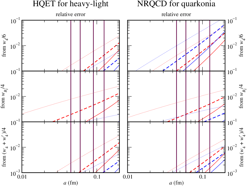
Figure 4: Relative truncation errors for the new action, from discretization effects that break rotational symmetry. The curves have the same meaning as in Fig. 3.

To drive these contributions to heavy-quark discretization effects below 1%, we again find it sufficient to tune the couplings of the new action at the tree level.

There are some other noteworthy features of Figs. 3 and 4. For $m_{Q}a\ll 1$, the discretization effects vanish as a power of $a$, as one would deduce from the Symanzik effective field theory. Because we identify $m_{2}$ with the mass in the ${\cal C}_{i}^{\mathrm{cont}}$, the powers of $a$ are balanced by $\Lambda$ or $m_{Q}\upsilon$, not $m_{Q}$. Had we identified $m_{1}$ with the physical mass, errors of order $(m_{Q}a)^{n}$ would have appeared. For $m_{Q}a\sim 1$, the tree-level curves flatten out. The error cannot grow without bound, because of the heavy-quark symmetries of the Wilson action and our improvements to it. Indeed, the curves for the $b$ quark are usually lower than those for the $c$ quark, which bodes well for calculations relevant to the Cabibbo-Kobayashi-Maskawa matrix. The underlying reason for the pattern is that the static approximation works better for $b$-flavored hadrons than for charmed hadrons. The $1/m_{b}^{n}$ contributions start out smaller, so their mismatches are also smaller. Similarly, the leading NRQCD works better for bottomonium than charmonium. The mismatches from $1/8m_{4}^{3}$ and $w_{4}/6$ deviate from the pattern, however, because NRQCD’s relative suppression $\upsilon^{2}_{\bar{b}b}/\upsilon^{2}_{\bar{c}c}$ is not as strong as HQET’s $(m_{c}/m_{b})^{3}$. Mismatches from $w_{B_{i}}/4$ and $(w_{4}+w^{\prime}_{4})/4$ are of order $\upsilon^{4}$ and again follow the pattern.

In tree-level improvement, one should avoid choices where it is known that one-loop corrections from tadpole diagrams will be large Lepage:1992xa . Therefore, we envision following some sort of tadpole improvement. In the action, write each link matrix as $u_{0}[U_{\mu}/u_{0}]$ and absorb all but one pre-factor of $u_{0}$ into a tadpole-improved coupling $\tilde{c}_{i}$ and $\tilde{r}_{i}$. (In several cases, it will be necessary to expand expressions such as ${D_{i}}_{\rm lat}{\triangle_{i}}_{\rm lat}$, ${\triangle_{i}}_{\rm lat}^{2}$, and Eq. (39), to eliminate any instance of $U_{\mu}U_{\mu}^{\dagger}=1$ before inserting $u_{0}$.) Then apply the conditions of Sec. IV to $\tilde{c}_{i}$ and $\tilde{r}_{i}$ instead of $c_{i}$ and $r_{i}$, and take the $u_{0}$ factors in the denominator from the Monte Carlo simulation.

VI Conclusions

In this paper we have presented the formalism and explicit calculations needed to define a new lattice action for heavy quarks. Our aim was to obtain an action whose discretization errors would be $\lesssim 1\%$ at currently available lattice spacings. Combining our matching calculations, power counting, and the heavy-quark theory of discretization effects, we have argued that the proposed action should meet its target. Setting to zero the redundant couplings and those that vanish when matched at the tree level, our action can be written $S=S_{0}+S_{B}+S_{E}+S_{\rm new}$, where

$$S_{\rm new} = c_{1}a^{6}\sum_{x}\bar{\psi}(x)\sum_{i}\gamma_{i}{D_{i}}_{\mathrm{lat}}{\triangle_{i}}_{\mathrm{lat}}\psi(x)+c_{2}a^{6}\sum_{x}\bar{\psi}(x)\{\bm{\gamma}\cdot\bm{D}_{\mathrm{lat}},\triangle^{(3)}_{\mathrm{lat}}\}\psi(x)$$ (123)

$$+ c_{3}a^{6}\sum_{x}\bar{\psi}(x)\{\bm{\gamma}\cdot\bm{D}_{\mathrm{lat}},i\bm{\Sigma}\cdot\bm{B}_{\mathrm{lat}}\}\psi(x)+c_{EE}a^{6}\sum_{x}\bar{\psi}(x)\{\gamma_{4}{D_{4}}_{\mathrm{lat}},\bm{\alpha}\cdot\bm{E}_{\mathrm{lat}}\}\psi(x)$$

$$+ c_{4}a^{7}\sum_{x}\bar{\psi}(x)\sum_{i}{\triangle_{i}}_{\mathrm{lat}}^{2}\psi(x)+c_{5}a^{7}\sum_{x}\bar{\psi}(x)\sum_{i}\sum_{j\neq i}\{i\Sigma_{i}{B_{i}}_{\mathrm{lat}},{\triangle_{j}}_{\mathrm{lat}}\}\psi(x).$$

The new action has six additional nonzero couplings, which depend on the couplings in $S_{0}+S_{B}+S_{E}$ according to Eqs. (113)–(116) and (119). To achieve 1% accuracy, $S_{B}$ must be, and $S_{E}$ could well be, matched at the one-loop level Nobes:2003nc .

Another lattice action achieves similar accuracy for charmed quarks, namely the highly-improved staggered quark (HISQ) action Follana:2006rc . Our approach is computationally more demanding than HISQ. Its advantage, however, is the intriguing result that our discretization errors for bottom quarks are smaller than for charmed quarks. That means that experience with charmed hadrons and charmonium can inform analogous calculation of properties of $b$-flavored hadrons.

Finally, we note that there is tension between the most accurate calculation of the $D_{s}$ meson decay constant, $f_{D_{s}}$ Follana:2007uv , which uses HISQ, and experimental measurements Dobrescu:2008fd . Our action is a candidate for the charmed quark in a cross-check of the HISQ $f_{D_{s}}$, because its discretization errors can be expected to be small enough to strengthen or dissipate the disagreement, while possessing different systematic errors.

Appendix A Feynman Rules

In this Appendix we present Feynman rules for the new action needed to carry out the matching calculations of Sec. IV. These are the quark and gluon propagators and three- and four-point vertices. The corresponding Feynman diagrams are shown in Fig. 5.

Figure 5: Feynman rules for the action $S$ given by Eqs. (29)–(35).

The quark propagator [Fig. 5(a)] is modified only through $c_{2}$, $c_{1}$, $z_{6}$, and $c_{4}$. It reads

$$aS^{-1}(p)=i\gamma_{4}\sin(p_{4}a)+i\bm{\gamma}\cdot\bm{K}(p)+\mu(p)-\cos(p_{4}a)$$ (124)

where

$$K_{i}(p) = \sin(p_{i}a)\left[\zeta-2c_{2}\hat{\bm{p}}^{2}a^{2}-c_{1}\hat{p}_{i}^{2}a^{2}\right]$$ (125)

$$\mu(p) = 1+m_{0}a+\hat{\bm{p}}^{2}a^{2}\left[{\textstyle\frac{1}{2}}r_{s}\zeta+z_{6}\hat{\bm{p}}^{2}a^{2}\right]+c_{4}\sum_{i}(\hat{p}_{i}a)^{4}$$ (126)

The tree-level mass shell is $p_{4}=iE$, where the energy satisfies

$$\cosh Ea=\frac{1+\mu^{2}+\bm{K}^{2}}{2\mu(\bm{p})}.$$ (127)

Incoming external fermion lines receive factors $u(\xi,\bm{p})\mathcal{N}(p)$ or $v(\xi,\bm{p})\mathcal{N}(p)$, where

$$\mathcal{N}(p) = \left(\frac{L}{\mu(\bm{p})\sinh E}\right)^{1/2},$$ (128)

$$u(\xi,\bm{p}) = \frac{L+\sinh E-i\bm{\gamma}\cdot\bm{K}}{\sqrt{2L(L+\sinh E)}}u(\xi,\bm{0}),$$ (129)

$$v(\xi,\bm{p}) = \frac{L+\sinh E+i\bm{\gamma}\cdot\bm{K}}{\sqrt{2L(L+\sinh E)}}v(\xi,\bm{0}),$$ (130)

$L=\mu(\bm{p})-\cosh E$; $\gamma_{4}u(\xi,\bm{0})=u(\xi,\bm{0})$, $\gamma_{4}v(\xi,\bm{0})=-v(\xi,\bm{0})$. Outgoing external fermion lines receive factors $\mathcal{N}(p)\bar{u}(\xi,\bm{p})$ or $\mathcal{N}(p)\bar{v}(\xi,\bm{p})$, where $\bar{u}(\xi,\bm{p})=u^{\dagger}(\xi,\bm{p})\gamma_{4}$, $\bar{v}(\xi,\bm{p})=v^{\dagger}(\xi,\bm{p})\gamma_{4}$.

The gluon propagator [Fig. 5(b)] is not easy to express in closed form. We refer the reader to two papers of Weisz for details Weisz:1982zw and a correction Weisz:1983bn for the propagator on isotropic lattices. The improved vertex is in Ref. Weisz:1983bn .

Now let us turn to vertices with one [Fig. 5(c)–(d)] or two [Fig. 5(e)–(g)] gluons attached to a quark line. The new terms in the bilinear part of the action are all built from difference and clover operators that already appear in $S_{0}+S_{B}+S_{E}$. Consequently, the new terms in the Feynman rules for these vertices can be obtained using the chain rule.

The difference operators are given in Eqs. (36)–(38). To simplify notation, let us drop the subscript “lat” in this Appendix. One-gluon vertices need

$${D_{\rho}}^{\;a}_{,\mu}(P,k)=\frac{\partial D_{\rho}}{\partial A^{a}_{\mu}(k)} = g_{0}t^{a}\delta_{\rho\mu}\cos[(P+{\textstyle\frac{1}{2}}k)_{\mu}a],$$ (131)

$${\triangle_{\rho}}^{\;a}_{,\mu}(P,k)=\frac{\partial\triangle_{\rho}}{\partial A^{a}_{\mu}(k)} = g_{0}t^{a}\delta_{\rho\mu}(2i/a)\sin[(P+{\textstyle\frac{1}{2}}k)_{\mu}a],$$ (132)

$${F_{\rho\sigma}}^{\;a}_{,\mu}(k)=\frac{\partial{F_{\rho\sigma}}}{\partial A^{a}_{\mu}(k)} = g_{0}t^{a}\cos{\textstyle\frac{1}{2}}k_{\mu}a\left[\delta_{\mu\sigma}iS_{\rho}(k)-\delta_{\mu\rho}iS_{\sigma}(k)\right].$$ (133)

It is convenient to write out the chromomagnetic and chromoelectric cases of Eq. (133):

$${B_{i}}^{\;a}_{,m}(k)=\frac{\partial{B_{i}}}{\partial A^{a}_{m}(k)} = -g_{0}t^{a}\cos({\textstyle\frac{1}{2}}k_{m}a)\varepsilon_{mri}iS_{r}(k),$$ (134)

$${E_{i}}^{\;a}_{,m}(k)=\frac{\partial{E_{i}}}{\partial A^{a}_{m}(k)} = g_{0}t^{a}\cos({\textstyle\frac{1}{2}}k_{m}a)\delta_{mi}iS_{4}(k),$$ (135)

$${E_{i}}^{\;a}_{,4}(k)=\frac{\partial{E_{i}}}{\partial A^{a}_{4}(k)} = -g_{0}t^{a}\cos({\textstyle\frac{1}{2}}k_{4}a)iS_{i}(k),$$ (136)

since $B_{i}={\textstyle\frac{1}{2}}\varepsilon_{ijk}F_{jk}$ and $E_{i}=F_{4i}$ appear in Eq. (29). Two-gluon vertices need

$${D_{\rho}}^{\;ab}_{,\mu\nu}(P,k,l)=\frac{\partial^{2}D_{\rho}}{\partial A^{a}_{\mu}(k)\partial A^{b}_{\nu}(l)} = g_{0}^{2}{\textstyle\frac{1}{2}}\{t^{a},t^{b}\}\delta_{\mu\nu}\delta_{\rho\mu}ai\sin[(P+{\textstyle\frac{1}{2}}K)_{\mu}a],$$ (137)

$${\triangle_{\rho}}^{\;ab}_{,\mu\nu}(P,k,l)=\frac{\partial^{2}\triangle_{\rho}}{\partial A^{a}_{\mu}(k)\partial A^{b}_{\nu}(l)} = g_{0}^{2}{\textstyle\frac{1}{2}}\{t^{a},t^{b}\}\delta_{\mu\nu}\delta_{\rho\mu}2\cos[(P+{\textstyle\frac{1}{2}}K)_{\mu}a],$$ (138)

where $K=k+l$. For the clover operator it is convenient to introduce

$$C_{\mu\nu}(k,l)=2\cos{\textstyle\frac{1}{2}}(k+l)_{\mu}a\cos{\textstyle\frac{1}{2}}l_{\mu}a\cos{\textstyle\frac{1}{2}}(k+l)_{\nu}a\cos{\textstyle\frac{1}{2}}k_{\nu}a-\cos{\textstyle\frac{1}{2}}k_{\mu}a\cos{\textstyle\frac{1}{2}}l_{\nu}a.$$ (139)

Then one has ($K=k+l$)

$${F_{\rho\sigma}}^{\;ab}_{,\mu\nu}(k,l)=\frac{\partial^{2}F_{\rho\sigma}}{\partial A^{a}_{\mu}(k)\partial A^{b}_{\nu}(l)} = g_{0}^{2}[t^{a},t^{b}]\left\{\vphantom{\hat{K}}(\delta_{\mu\rho}\delta_{\nu\sigma}-\delta_{\mu\sigma}\delta_{\nu\rho})C_{\mu\nu}(k,l)\right.$$

$$- \left.{\textstyle\frac{1}{4}}\delta_{\mu\nu}a^{2}\hat{K}_{\mu}\left[\delta_{\mu\rho}\left(S_{\sigma}(k)-S_{\sigma}(l)\right)-\delta_{\mu\sigma}\left(S_{\rho}(k)-S_{\rho}(l)\right)\right]\right\},$$

$${B_{i}}^{\;ab}_{,mn}(k,l)=\frac{\partial^{2}{B_{i}}}{\partial A^{a}_{m}(k)\partial A^{b}_{n}(l)} = g_{0}^{2}[t^{a},t^{b}]\left\{\varepsilon_{mni}C_{mn}(k,l)-{\textstyle\frac{1}{4}}\delta_{mn}\varepsilon_{mri}a^{2}\hat{K}_{m}\left[S_{r}(k)-S_{r}(l)\right]\right\},$$

$${E_{i}}^{\;ab}_{,mn}(k,l)=\frac{\partial^{2}{E_{i}}}{\partial A^{a}_{m}(k)\partial A^{b}_{n}(l)} = g_{0}^{2}[t^{a},t^{b}]{\textstyle\frac{1}{4}}\delta_{mn}\delta_{mi}a^{2}\hat{K}_{m}\left[S_{4}(k)-S_{4}(l)\right],$$ (142)

$${E_{i}}^{\;ab}_{,4n}(k,l)=\frac{\partial^{2}{E_{i}}}{\partial A^{a}_{4}(k)\partial A^{b}_{n}(l)} = g_{0}^{2}[t^{a},t^{b}]\delta_{ni}C_{4n}(k,l),$$ (143)

$${E_{i}}^{\;ab}_{,44}(k,l)=\frac{\partial^{2}{E_{i}}}{\partial A^{a}_{4}(k)\partial A^{b}_{4}(l)} = -g_{0}^{2}[t^{a},t^{b}]{\textstyle\frac{1}{4}}a^{2}\hat{K}_{4}\left[S_{i}(k)-S_{i}(l)\right].$$ (144)

The Feynman rules for one gluon are then

$${\rm Fig.~{}\ref{fig:feynman}(c,d)}=-g_{0}t^{a}_{ij}\Lambda_{\mu}(p^{\prime},p),$$ (145)

with

$$\Lambda_{4}(p^{\prime},p) = \gamma_{4}\cos[{\textstyle\frac{1}{2}}(p^{\prime}+p)_{4}a]-i\sin[{\textstyle\frac{1}{2}}(p^{\prime}+p)_{4}a]+{\textstyle\frac{i}{2}}c_{E}\zeta a\bm{\alpha}\cdot\bm{S}(k)\cos({\textstyle\frac{1}{2}}k_{4}a)$$ (146)

$$+ ir_{E}a^{2}\gamma_{4}\bm{\Sigma}\cdot\left\{\bm{S}(k)\times\left[\bm{S}(p^{\prime})+\bm{S}(p)\right]\right\}\cos({\textstyle\frac{1}{2}}k_{4}a)$$

$$- (r_{E}-z_{E})a^{2}\gamma_{4}\bm{S}(k)\cdot\left[\bm{S}(p^{\prime})-\bm{S}(p)\right]\cos({\textstyle\frac{1}{2}}k_{4}a)$$

$$+ c_{EE}a^{2}\bm{\gamma}\cdot\bm{S}(k)\left[S_{4}(p^{\prime})-S_{4}(p)\right]\cos({\textstyle\frac{1}{2}}k_{4}a),$$

$$\Lambda_{m}(p^{\prime},p) = \zeta\gamma_{m}\cos[{\textstyle\frac{1}{2}}(p^{\prime}+p)_{m}a]-ir_{s}\zeta\sin[{\textstyle\frac{1}{2}}(p^{\prime}+p)_{m}a]$$ (147)

$$- {\textstyle\frac{1}{2}}c_{B}\zeta a\varepsilon_{mri}\Sigma_{i}S_{r}(k)\cos({\textstyle\frac{1}{2}}k_{m}a)-{\textstyle\frac{i}{2}}c_{E}\zeta a\alpha_{m}S_{4}(k)\cos({\textstyle\frac{1}{2}}k_{m}a)$$

$$- ir_{E}a^{2}\varepsilon_{mri}\Sigma_{i}\gamma_{4}S_{4}(k)\left[S_{r}(p^{\prime})+S_{r}(p)\right]\cos({\textstyle\frac{1}{2}}k_{m}a)$$

$$+ (r_{E}-z_{E})a^{2}\gamma_{4}S_{4}(k)\left[S_{m}(p^{\prime})-S_{m}(p)\right]\cos({\textstyle\frac{1}{2}}k_{m}a)$$

$$- c_{2}a^{2}\left\{\gamma_{m}\cos[{\textstyle\frac{1}{2}}(p^{\prime}+p)_{m}a]\left(\widehat{\bm{p}^{\prime}}^{2}+\hat{\bm{p}}^{2}\right)+\bm{\gamma}\cdot\left[\bm{S}(p^{\prime})+\bm{S}(p)\right]\widehat{(p^{\prime}+p)}_{m}\right\}$$

$$- {\textstyle\frac{1}{2}}c_{1}a^{2}\gamma_{m}\left\{\cos[{\textstyle\frac{1}{2}}(p^{\prime}+p)_{m}a]\left(\widehat{p_{m}^{\prime}}^{2}+\hat{p}_{m}^{2}\right)+\left[S_{m}(p^{\prime})+S_{m}(p)\right]\widehat{(p^{\prime}+p)}_{m}\right\}$$

$$- c_{3}a^{2}\varepsilon_{mri}\gamma_{4}\gamma_{5}S_{r}(k)\left[S_{i}(p^{\prime})+S_{i}(p)\right]\cos({\textstyle\frac{1}{2}}k_{m}a)$$

$$+ (c_{3}-z_{3})a^{2}\bm{\gamma}\cdot\bm{S}(k)\left[S_{m}(p^{\prime})-S_{m}(p)\right]\cos({\textstyle\frac{1}{2}}k_{m}a)$$

$$- (c_{3}-z_{3})a^{2}\gamma_{m}\bm{S}(k)\cdot\left[\bm{S}(p^{\prime})-\bm{S}(p)\right]\cos({\textstyle\frac{1}{2}}k_{m}a)$$

$$- c_{EE}a^{2}\gamma_{m}S_{4}(k)\left[S_{4}(p^{\prime})-S_{4}(p)\right]\cos({\textstyle\frac{1}{2}}k_{m}a)$$

$$- iz_{6}a^{3}\widehat{(p^{\prime}+p)}_{m}\left(\widehat{\bm{p}^{\prime}}^{2}+\hat{\bm{p}}^{2}\right)$$

$$- ic_{4}a^{3}\widehat{(p^{\prime}+p)}_{m}\left(\widehat{p_{m}^{\prime}}^{2}+\hat{p}_{m}^{2}\right)$$

$$- (z_{7}+c_{5})a^{3}\varepsilon_{mri}\Sigma_{i}S_{r}(k)\left(\hat{\bm{p}^{\prime}}^{2}+\hat{\bm{p}}^{2}\right)\cos({\textstyle\frac{1}{2}}k_{m}a)$$

$$+ c_{5}a^{3}\varepsilon_{mri}\Sigma_{i}S_{r}(k)\left(\hat{p^{\prime}}_{i}^{2}+\hat{p}_{i}^{2}\right)\cos({\textstyle\frac{1}{2}}k_{m}a)$$

$$+ r_{5}a^{3}\varepsilon_{mri}\Sigma_{i}S_{r}(k)\left[S_{i}(p^{\prime})S_{i}(p)\right]\cos({\textstyle\frac{1}{2}}k_{m}a)$$

$$+ (r_{7}-z^{\prime}_{7}-r_{5})a^{3}\varepsilon_{mri}\Sigma_{i}S_{r}(k)\left[\bm{S}(p^{\prime})\cdot\bm{S}(p)\right]\cos({\textstyle\frac{1}{2}}k_{m}a)$$

$$- r_{7}a^{3}\varepsilon_{mri}\left[S_{i}(p^{\prime})\bm{\Sigma}\cdot\bm{S}(p)+S_{i}(p)\bm{\Sigma}\cdot\bm{S}(p)\right]S_{r}(k)\cos({\textstyle\frac{1}{2}}k_{m}a)$$

$$+ i(r_{7}-r^{\prime}_{7})a^{3}\left[S_{m}(p^{\prime})\bm{S}(p)\cdot\bm{S}(k)-S_{m}(p)\bm{S}(p^{\prime})\cdot\bm{S}(k)\right]\cos({\textstyle\frac{1}{2}}k_{m}a).$$

In the $r_{5}$ and $z^{\prime}_{7}$ terms, Eq. (39) has been assumed. If instead one prefers Eq. (40) then replace

$$\left[S_{j}(p^{\prime})S_{j}(p)\right]\to\left[\cos({\textstyle\frac{1}{2}}k_{j}a)\hat{p}^{\prime}_{j}\hat{p}_{j}\right].$$

Both choices have the same effect on Eq. (61).

The two-gluon rules are

$${\rm Fig.~{}\ref{fig:feynman}(e,f,g)}=-{\textstyle\frac{1}{2}}g_{0}^{2}\{t^{a},t^{b}\}_{ij}aX_{\mu\nu}(p,k,l)-{\textstyle\frac{1}{2}}g_{0}^{2}[t^{a},t^{b}]_{ij}aY_{\mu\nu}(p,k,l),$$ (148)

with

$$X_{mn}(p,k,l) = i\zeta\delta_{mn}\gamma_{m}\sin({\textstyle\frac{1}{2}}s_{m}a)-r_{s}\zeta\delta_{mn}\cos({\textstyle\frac{1}{2}}s_{m}a)$$ (149)

$$- 2r_{E}a\varepsilon_{mni}\gamma_{4}\Sigma_{i}\left[\cos({\textstyle\frac{1}{2}}s_{n}a)\cos({\textstyle\frac{1}{2}}k_{n}a)\cos({\textstyle\frac{1}{2}}k_{m}a)S_{4}(k)\right.$$

$$\quad-\left.\cos({\textstyle\frac{1}{2}}s_{m}a)\cos({\textstyle\frac{1}{2}}l_{m}a)\cos({\textstyle\frac{1}{2}}l_{n}a)S_{4}(l)\right]$$

$$+ i(r_{E}-z_{E})a^{2}\gamma_{4}\delta_{mn}\sin({\textstyle\frac{1}{2}}s_{m}a)\left[S_{m}(k)S_{4}(k)+S_{m}(l)S_{4}(l)\right]$$

$$+ 4ic_{2}\gamma_{m}\left[\cos({\textstyle\frac{1}{2}}s_{m}a)\cos({\textstyle\frac{1}{2}}l_{m}a)\sin({\textstyle\frac{1}{2}}s_{n}a)\cos({\textstyle\frac{1}{2}}k_{n}a)\right.$$

$$\quad+\,\left.\sin({\textstyle\frac{1}{2}}s_{m}a)\sin({\textstyle\frac{1}{2}}l_{m}a)\cos({\textstyle\frac{1}{2}}s_{n}a)\sin({\textstyle\frac{1}{2}}k_{n}a)\right]$$

$$+ 4ic_{2}\gamma_{n}\left[\sin({\textstyle\frac{1}{2}}s_{m}a)\cos({\textstyle\frac{1}{2}}l_{m}a)\cos({\textstyle\frac{1}{2}}s_{n}a)\cos({\textstyle\frac{1}{2}}k_{n}a)\right.$$

$$\quad+\,\left.\cos({\textstyle\frac{1}{2}}s_{m}a)\sin({\textstyle\frac{1}{2}}l_{m}a)\sin({\textstyle\frac{1}{2}}s_{n}a)\sin({\textstyle\frac{1}{2}}k_{n}a)\right]$$

$$+ 2ic_{2}a\delta_{mn}\cos({\textstyle\frac{1}{2}}s_{m}a)\,\bm{\gamma}\cdot\left[\bm{S}(p^{\prime})+\bm{S}(p)\right]$$

$$- ic_{2}a^{2}\delta_{mn}\gamma_{m}\sin({\textstyle\frac{1}{2}}s_{m}a)\left(\widehat{\bm{p}^{\prime}}^{2}+\hat{\bm{p}}^{2}\right)$$

$$+ ic_{1}a\delta_{mn}\gamma_{m}\hat{s}_{m}\left[4\cos({\textstyle\frac{1}{2}}s_{m}a)\cos({\textstyle\frac{1}{2}}k_{m}a)\cos({\textstyle\frac{1}{2}}l_{m}a)-1\right]$$

$$+ 2ic_{3}\varepsilon_{mnr}\gamma_{4}\gamma_{5}\left[\sin(l_{r}a)\cos({\textstyle\frac{1}{2}}s_{m}a)\cos({\textstyle\frac{1}{2}}l_{m}a)\cos({\textstyle\frac{1}{2}}l_{n}a)\right.$$

$$\quad-\left.\sin(k_{r}a)\cos({\textstyle\frac{1}{2}}s_{n}a)\cos({\textstyle\frac{1}{2}}k_{n}a)\cos({\textstyle\frac{1}{2}}k_{m}a)\right]$$

$$+ 2i(c_{3}-z_{3})a\left\{[\delta_{mn}\bm{\gamma}\cdot\bm{S}(l)-\gamma_{n}S_{m}(l)]\sin({\textstyle\frac{1}{2}}s_{m}a)\sin({\textstyle\frac{1}{2}}l_{m}a)\cos({\textstyle\frac{1}{2}}l_{n}a)\right.$$

$$\quad+\left.[\delta_{mn}\bm{\gamma}\cdot\bm{S}(k)-\gamma_{m}S_{n}(k)]\sin({\textstyle\frac{1}{2}}s_{n}a)\sin({\textstyle\frac{1}{2}}k_{n}a)\cos({\textstyle\frac{1}{2}}k_{m}a)\right\}$$

$$- 8z_{6}\left[\sin({\textstyle\frac{1}{2}}s_{m}a)\cos({\textstyle\frac{1}{2}}l_{m}a)\sin({\textstyle\frac{1}{2}}s_{n}a)\cos({\textstyle\frac{1}{2}}k_{n}a)\right.$$

$$\quad-\left.\cos({\textstyle\frac{1}{2}}s_{m}a)\sin({\textstyle\frac{1}{2}}l_{m}a)\cos({\textstyle\frac{1}{2}}s_{n}a)\sin({\textstyle\frac{1}{2}}k_{n}a)\right]$$

$$- 2z_{6}a^{2}\delta_{mn}\cos({\textstyle\frac{1}{2}}s_{m}a)\left(\widehat{\bm{p}^{\prime}}^{2}+\hat{\bm{p}}^{2}\right)$$

$$- 2c_{4}a^{2}\delta_{mn}\left\{\cos({\textstyle\frac{1}{2}}s_{m}a)\left(\widehat{p^{\prime}}_{m}^{2}+\hat{p}_{m}^{2}\right)+\cos[{\textstyle\frac{1}{2}}(k-l)_{m}a]\hat{s}_{m}^{2}-\hat{k}_{m}\hat{l}_{m}\right\}$$

$$+ 2i(z_{7}+c_{5})a^{2}\Sigma_{i}\left[\hat{s}_{n}\varepsilon_{mri}S_{r}(k)\cos({\textstyle\frac{1}{2}}k_{m}a)\cos({\textstyle\frac{1}{2}}k_{n}a)\right.$$

$$\quad+\left.\hat{s}_{m}\varepsilon_{nri}S_{r}(l)\cos({\textstyle\frac{1}{2}}l_{n}a)\cos({\textstyle\frac{1}{2}}l_{m}a)\right]$$

$$+ 2ic_{5}a^{2}\varepsilon_{mnr}\left[\hat{s}_{n}\Sigma_{n}S_{r}(k)\cos({\textstyle\frac{1}{2}}k_{m}a)\cos({\textstyle\frac{1}{2}}k_{n}a)\right.$$

$$\quad-\left.\hat{s}_{m}\Sigma_{m}S_{r}(l)\cos({\textstyle\frac{1}{2}}l_{n}a)\cos({\textstyle\frac{1}{2}}l_{m}a)\right]$$

$$+ ir_{5}a^{2}\varepsilon_{mnr}\left\{\Sigma_{n}S_{n}(s)S_{r}(k)-\Sigma_{m}S_{m}(s)S_{r}(l)\right\}\cos({\textstyle\frac{1}{2}}k_{m}a)\cos({\textstyle\frac{1}{2}}l_{n}a)$$

$$+ ir_{7}a^{2}\Sigma_{n}\varepsilon_{mri}S_{r}(k)\left\{\left[S_{i}(p^{\prime})+S_{i}(p)\right]\cos({\textstyle\frac{1}{2}}s_{n}a)\cos({\textstyle\frac{1}{2}}k_{n}a)\right.$$

$$\quad+\left.\left[S_{i}(p^{\prime})-S_{i}(p)\right]\sin({\textstyle\frac{1}{2}}s_{n}a)\sin({\textstyle\frac{1}{2}}k_{n}a)\right\}\cos({\textstyle\frac{1}{2}}k_{m}a)$$

$$+ ir_{7}a^{2}\Sigma_{m}\varepsilon_{nri}S_{r}(l)\left\{\left[S_{i}(p^{\prime})+S_{i}(p)\right]\cos({\textstyle\frac{1}{2}}s_{m}a)\cos({\textstyle\frac{1}{2}}l_{m}a)\right.$$

$$\quad+\left.\left[S_{i}(p^{\prime})-S_{i}(p)\right]\sin({\textstyle\frac{1}{2}}s_{m}a)\sin({\textstyle\frac{1}{2}}l_{m}a)\right\}\cos({\textstyle\frac{1}{2}}l_{n}a)$$

$$- ir_{7}a^{2}\varepsilon_{mnr}S_{r}(k)\bm{\Sigma}\cdot\left\{\left[\bm{S}(p^{\prime})+\bm{S}(p)\right]\cos({\textstyle\frac{1}{2}}s_{n}a)\cos({\textstyle\frac{1}{2}}k_{n}a)\right.$$

$$\quad+\left.\left[\bm{S}(p^{\prime})-\bm{S}(p)\right]\sin({\textstyle\frac{1}{2}}s_{n}a)\sin({\textstyle\frac{1}{2}}k_{n}a)\right\}\cos({\textstyle\frac{1}{2}}k_{m}a)$$

$$+ ir_{7}a^{2}\varepsilon_{mnr}S_{r}(l)\bm{\Sigma}\cdot\left\{\left[\bm{S}(p^{\prime})+\bm{S}(p)\right]\cos({\textstyle\frac{1}{2}}s_{m}a)\cos({\textstyle\frac{1}{2}}l_{m}a)\right.$$

$$\quad+\left.\left[\bm{S}(p^{\prime})-\bm{S}(p)\right]\sin({\textstyle\frac{1}{2}}s_{m}a)\sin({\textstyle\frac{1}{2}}l_{m}a)\right\}\cos({\textstyle\frac{1}{2}}l_{n}a)$$

$$+ i(z^{\prime}_{7}+r_{5}-r_{7})a^{2}\varepsilon_{mri}S_{n}(s)\Sigma_{i}S_{r}(k)\cos({\textstyle\frac{1}{2}}k_{m}a)\cos({\textstyle\frac{1}{2}}l_{n}a)$$

$$+ i(z^{\prime}_{7}+r_{5}-r_{7})a^{2}\varepsilon_{nri}S_{m}(s)\Sigma_{i}S_{r}(l)\cos({\textstyle\frac{1}{2}}k_{m}a)\cos({\textstyle\frac{1}{2}}l_{n}a)$$

$$- (r^{\prime}_{7}-r_{7})a^{2}S_{n}(k)\left[S_{m}(p^{\prime})-S_{m}(p)\right]\cos({\textstyle\frac{1}{2}}s_{n}a)\cos({\textstyle\frac{1}{2}}k_{n}a)\cos({\textstyle\frac{1}{2}}k_{m}a)$$

$$- (r^{\prime}_{7}-r_{7})a^{2}S_{m}(l)\left[S_{n}(p^{\prime})-S_{n}(p)\right]\cos({\textstyle\frac{1}{2}}s_{m}a)\cos({\textstyle\frac{1}{2}}l_{m}a)\cos({\textstyle\frac{1}{2}}l_{n}a)$$

$$- (r^{\prime}_{7}-r_{7})a^{2}S_{n}(k)\left[S_{m}(p^{\prime})+S_{m}(p)\right]\sin({\textstyle\frac{1}{2}}s_{n}a)\sin({\textstyle\frac{1}{2}}k_{n}a)\cos({\textstyle\frac{1}{2}}k_{m}a)$$

$$- (r^{\prime}_{7}-r_{7})a^{2}S_{m}(l)\left[S_{n}(p^{\prime})+S_{n}(p)\right]\sin({\textstyle\frac{1}{2}}s_{m}a)\sin({\textstyle\frac{1}{2}}l_{m}a)\cos({\textstyle\frac{1}{2}}l_{n}a)$$

$$+ (r^{\prime}_{7}-r_{7})a^{2}\delta_{mn}\bm{S}(k)\cdot\left[\bm{S}(p^{\prime})-\bm{S}(p)\right]\cos({\textstyle\frac{1}{2}}s_{m}a)\cos^{2}({\textstyle\frac{1}{2}}k_{m}a)$$

$$+ (r^{\prime}_{7}-r_{7})a^{2}\delta_{mn}\bm{S}(l)\cdot\left[\bm{S}(p^{\prime})-\bm{S}(p)\right]\cos({\textstyle\frac{1}{2}}s_{m}a)\cos^{2}({\textstyle\frac{1}{2}}l_{m}a)$$

$$+ {\textstyle\frac{1}{4}}(r^{\prime}_{7}-r_{7})a^{4}\delta_{mn}\hat{s}_{m}\left\{S_{m}(k)\bm{S}(k)+S_{m}(l)\bm{S}(l)\right\}\cdot\left[\bm{S}(p^{\prime})+\bm{S}(p)\right]$$

$$+ 2(r_{BB}-z_{BB})a^{2}\left[\delta_{mn}\bm{S}(k)\cdot\bm{S}(l)-S_{m}(l)S_{n}(k)\right]\cos({\textstyle\frac{1}{2}}k_{m}a)\cos({\textstyle\frac{1}{2}}l_{n}a)$$

$$- 2(r_{EE}+z_{EE})a^{2}\delta_{mn}S_{4}(k)S_{4}(l)\cos({\textstyle\frac{1}{2}}k_{m}a)\cos({\textstyle\frac{1}{2}}l_{n}a),$$

where now $p^{\prime}=p+k+l$, and $s=p^{\prime}+p=2p+k+l$;

$$X_{44}(p,k,l) = i\gamma_{4}\sin[{\textstyle\frac{1}{2}}(p^{\prime}+p)_{4}a]-\cos[{\textstyle\frac{1}{2}}(p^{\prime}+p)_{4}a]$$ (150)

$$+ ic_{EE}a^{2}\left[\bm{\gamma}\cdot\bm{S}(k)S_{4}(k)+\bm{\gamma}\cdot\bm{S}(l)S_{4}(l)\right]\sin[{\textstyle\frac{1}{2}}(p^{\prime}+p)_{4}a]$$

$$- 2(r_{EE}+z_{EE})a^{2}\bm{S}(k)\cdot\bm{S}(l)\cos({\textstyle\frac{1}{2}}k_{4}a)\cos({\textstyle\frac{1}{2}}l_{4}a),$$

$$X_{4m}(p,k,l) = -2r_{E}a\varepsilon_{mri}\gamma_{4}\Sigma_{i}S_{r}(k)\cos({\textstyle\frac{1}{2}}s_{m}a)\cos({\textstyle\frac{1}{2}}k_{4}a)\cos({\textstyle\frac{1}{2}}k_{m}a)$$ (151)

$$- i(r_{E}-z_{E})a^{2}\gamma_{4}\hat{k}_{m}^{2}\sin({\textstyle\frac{1}{2}}s_{m}a)\cos({\textstyle\frac{1}{2}}k_{4}a)\cos({\textstyle\frac{1}{2}}k_{m}a)$$

$$- ic_{EE}a^{2}\gamma_{m}\hat{l}_{4}^{2}\sin[{\textstyle\frac{1}{2}}(p^{\prime}+p)_{4}a]\cos({\textstyle\frac{1}{2}}l_{4}a)\cos({\textstyle\frac{1}{2}}l_{m}a)$$

$$+ 2(r_{EE}+z_{EE})a^{2}S_{m}(k)S_{4}(l)\cos({\textstyle\frac{1}{2}}k_{4}a)\cos({\textstyle\frac{1}{2}}l_{m}a),$$

$$Y_{mn}(p,k,l) = -ic_{B}\zeta\Sigma_{i}\bar{C}_{mni}(k,l)-{\textstyle\frac{1}{4}}c_{E}\zeta a^{2}\delta_{mn}\alpha_{m}\hat{K}_{m}\left[S_{4}(k)-S_{4}(l)\right]$$ (152)

$$- {\textstyle\frac{1}{2}}r_{E}a^{3}\varepsilon_{mni}\gamma_{4}\Sigma_{i}\left[\hat{s}_{n}\hat{k}_{n}S_{4}(k)\cos({\textstyle\frac{1}{2}}k_{m}a)+\hat{s}_{m}\hat{l}_{m}S_{4}(l)\cos({\textstyle\frac{1}{2}}l_{n}a)\right]$$

$$- {\textstyle\frac{1}{2}}r_{E}a^{3}\delta_{mn}\varepsilon_{mri}\gamma_{4}\Sigma_{i}\hat{K}_{m}[S_{r}(p^{\prime})+S_{r}(p)][S_{4}(k)-S_{4}(l)]$$

$$+ 2i(r_{E}-z_{E})a\delta_{mn}\gamma_{4}\left[S_{4}(k)\cos^{2}({\textstyle\frac{1}{2}}k_{m}a)-S_{4}(l)\cos^{2}({\textstyle\frac{1}{2}}l_{m}a)\right]\cos({\textstyle\frac{1}{2}}s_{m}a)$$

$$- {\textstyle\frac{i}{2}}(r_{E}-z_{E})a^{3}\gamma_{4}\delta_{mn}\hat{K}_{m}[S_{m}(p^{\prime})-S_{m}(p)][S_{4}(k)-S_{4}(l)]$$

$$- 4ic_{2}\gamma_{m}\left[\cos({\textstyle\frac{1}{2}}s_{m}a)\cos({\textstyle\frac{1}{2}}l_{m}a)\cos({\textstyle\frac{1}{2}}s_{n}a)\sin({\textstyle\frac{1}{2}}k_{n}a)\right.$$

$$\quad+\,\left.\sin({\textstyle\frac{1}{2}}s_{m}a)\sin({\textstyle\frac{1}{2}}l_{m}a)\sin({\textstyle\frac{1}{2}}s_{n}a)\cos({\textstyle\frac{1}{2}}k_{n}a)\right]$$

$$+ 4ic_{2}\gamma_{n}\left[\cos({\textstyle\frac{1}{2}}s_{n}a)\cos({\textstyle\frac{1}{2}}k_{n}a)\cos({\textstyle\frac{1}{2}}s_{m}a)\sin({\textstyle\frac{1}{2}}l_{m}a)\right.$$

$$\quad+\,\left.\sin({\textstyle\frac{1}{2}}s_{n}a)\sin({\textstyle\frac{1}{2}}k_{n}a)\sin({\textstyle\frac{1}{2}}s_{m}a)\cos({\textstyle\frac{1}{2}}l_{m}a)\right]$$

$$- 2c_{1}\delta_{mn}i\gamma_{m}\cos[(p^{\prime}+p)_{m}a]\sin[{\textstyle\frac{1}{2}}(k-l)_{m}a]$$

$$- 2ic_{3}a\gamma_{4}\gamma_{5}\bar{C}_{mni}(k,l)[S_{i}(p^{\prime})+S_{i}(p)]$$

$$- {\textstyle\frac{i}{4}}c_{3}a^{3}\gamma_{4}\gamma_{5}\varepsilon_{mnr}\left[\hat{k}_{r}\hat{k}_{n}\hat{s}_{n}\cos({\textstyle\frac{1}{2}}k_{m}a)+\hat{l}_{r}\hat{l}_{m}\hat{s}_{m}\cos({\textstyle\frac{1}{2}}l_{n}a)\right]$$

$$- 2i(c_{3}-z_{3})a\left(\vphantom{\hat{K}_{m}}C_{mn}(k,l)\left\{\gamma_{m}[S_{n}(p^{\prime})-S_{n}(p)]-\gamma_{n}[S_{m}(p^{\prime})-S_{m}(p)]\right\}\right.$$

$$+\left.{\textstyle\frac{1}{4}}\delta_{mn}a^{2}\hat{K}_{m}[S_{m}(p^{\prime})-S_{m}(p)]\bm{\gamma}\cdot[\bm{S}(k)-\bm{S}(l)]\right.$$

$$-\left.{\textstyle\frac{1}{4}}\delta_{mn}\gamma_{m}a^{2}\hat{K}_{m}[\bm{S}(p^{\prime})-\bm{S}(p)]\cdot[\bm{S}(k)-\bm{S}(l)]\right.$$

$$+\left.[\delta_{mn}\bm{\gamma}\cdot\bm{S}(l)-\gamma_{n}S_{m}(l)]\cos({\textstyle\frac{1}{2}}s_{m}a)\cos({\textstyle\frac{1}{2}}l_{m}a)\cos({\textstyle\frac{1}{2}}l_{n}a)\right.$$

$$-\left.[\delta_{mn}\bm{\gamma}\cdot\bm{S}(k)-\gamma_{m}S_{n}(k)]\cos({\textstyle\frac{1}{2}}s_{n}a)\cos({\textstyle\frac{1}{2}}k_{n}a)\cos({\textstyle\frac{1}{2}}k_{m}a)\vphantom{\hat{K}_{m}}\right)$$

$$+ {\textstyle\frac{i}{2}}c_{EE}a^{3}\gamma_{m}\delta_{mn}\hat{K}_{m}\left[S_{4}(p^{\prime})-S_{4}(p)\right]\left[S_{4}(k)-S_{4}(l)\right]$$

$$- 2z_{6}a^{2}\left[\cos({\textstyle\frac{1}{2}}s_{m}a)\hat{l}_{m}\hat{s}_{n}\cos({\textstyle\frac{1}{2}}k_{n}a)-\cos({\textstyle\frac{1}{2}}s_{n}a)\hat{k}_{n}\hat{s}_{m}\cos({\textstyle\frac{1}{2}}l_{m}a)\right]$$

$$+ 4c_{4}\delta_{mn}\sin[(p^{\prime}+p)_{m}a]\sin[{\textstyle\frac{1}{2}}(k-l)_{m}a]$$

$$- 2i(z_{7}+c_{5})a^{2}\Sigma_{i}\left[\varepsilon_{mri}S_{r}(k)\hat{k}_{n}\cos({\textstyle\frac{1}{2}}s_{n}a)\cos({\textstyle\frac{1}{2}}k_{m}a)\right.$$

$$\quad-\left.\varepsilon_{nri}S_{r}(l)\hat{l}_{m}\cos({\textstyle\frac{1}{2}}s_{m}a)\cos({\textstyle\frac{1}{2}}l_{n}a)+\bar{C}_{mni}(k,l)\left(\widehat{\bm{p}^{\prime}}^{2}+\hat{\bm{p}}^{2}\right)\right]$$

$$- 2ic_{5}a^{2}\varepsilon_{mnr}\left[\Sigma_{n}S_{r}(k)\hat{k}_{n}\cos({\textstyle\frac{1}{2}}s_{n}a)\cos({\textstyle\frac{1}{2}}k_{m}a)\right.$$

$$\quad+\left.\Sigma_{m}S_{r}(l)\hat{l}_{m}\cos({\textstyle\frac{1}{2}}s_{m}a)\cos({\textstyle\frac{1}{2}}l_{n}a)\right]$$

$$+ 2ic_{5}a^{2}\Sigma_{i}\left(\widehat{p^{\prime}}_{i}^{2}+\hat{p}_{i}^{2}\right)\bar{C}_{mni}(k,l)$$

$$+ ir_{5}a^{2}\varepsilon_{mnr}\Sigma_{n}\left[\hat{K}_{n}\cos({\textstyle\frac{1}{2}}l_{n}a)-\hat{l}_{n}\sin^{2}({\textstyle\frac{1}{2}}s_{n}a)\right]S_{r}(k)\cos({\textstyle\frac{1}{2}}k_{m}a)$$

$$+ ir_{5}a^{2}\varepsilon_{mnr}\Sigma_{m}\left[\hat{K}_{m}\cos({\textstyle\frac{1}{2}}k_{m}a)-\hat{k}_{m}\sin^{2}({\textstyle\frac{1}{2}}s_{m}a)\right]S_{r}(l)\cos({\textstyle\frac{1}{2}}l_{n}a)$$

$$+ 2ir_{5}a^{2}\Sigma_{i}S_{i}(p^{\prime})S_{i}(p)\bar{C}_{mni}(k,l)$$

$$+ ir_{7}a^{2}\Sigma_{n}\varepsilon_{mri}S_{r}(k)\left\{\left[S_{i}(p^{\prime})-S_{i}(p)\right]\cos({\textstyle\frac{1}{2}}s_{n}a)\cos({\textstyle\frac{1}{2}}k_{n}a)\right.$$

$$\quad+\left.\left[S_{i}(p^{\prime})+S_{i}(p)\right]\sin({\textstyle\frac{1}{2}}s_{n}a)\sin({\textstyle\frac{1}{2}}k_{n}a)\right\}\cos({\textstyle\frac{1}{2}}k_{m}a)$$

$$- ir_{7}a^{2}\Sigma_{m}\varepsilon_{nri}S_{r}(l)\left\{\left[S_{i}(p^{\prime})-S_{i}(p)\right]\cos({\textstyle\frac{1}{2}}s_{m}a)\cos({\textstyle\frac{1}{2}}l_{m}a)\right.$$

$$\quad+\left.\left[S_{i}(p^{\prime})+S_{i}(p)\right]\sin({\textstyle\frac{1}{2}}s_{m}a)\sin({\textstyle\frac{1}{2}}l_{m}a)\right\}\cos({\textstyle\frac{1}{2}}l_{n}a)$$

$$- ir_{7}a^{2}\varepsilon_{mnr}S_{r}(k)\left\{\bm{\Sigma}\cdot\left[\bm{S}(p^{\prime})-\bm{S}(p)\right]\cos({\textstyle\frac{1}{2}}s_{m}a)\cos({\textstyle\frac{1}{2}}k_{m}a)\right.$$

$$\quad+\left.\bm{\Sigma}\cdot\left[\bm{S}(p^{\prime})+\bm{S}(p)\right]\sin({\textstyle\frac{1}{2}}s_{m}a)\sin({\textstyle\frac{1}{2}}k_{m}a)\right\}\cos({\textstyle\frac{1}{2}}k_{m}a)$$

$$- ir_{7}a^{2}\varepsilon_{mnr}S_{r}(l)\left\{\bm{\Sigma}\cdot\left[\bm{S}(p^{\prime})-\bm{S}(p)\right]\cos({\textstyle\frac{1}{2}}s_{n}a)\cos({\textstyle\frac{1}{2}}l_{n}a)\right.$$

$$\quad+\left.\bm{\Sigma}\cdot\left[\bm{S}(p^{\prime})+\bm{S}(p)\right]\sin({\textstyle\frac{1}{2}}s_{n}a)\sin({\textstyle\frac{1}{2}}l_{n}a)\right\}\cos({\textstyle\frac{1}{2}}l_{n}a)$$

$$- 2ir_{7}a^{2}\bm{\Sigma}\cdot\left[\bm{S}(p^{\prime})S_{i}(p)+\bm{S}(p)S_{i}(p^{\prime})\right]\bar{C}_{mni}(k,l)$$

$$+ i(z^{\prime}_{7}+r_{5}-r_{7})a^{2}\varepsilon_{mri}S_{r}(k)\Sigma_{i}\left\{\hat{K}_{n}\cos({\textstyle\frac{1}{2}}l_{n}a)-\hat{l}_{n}\sin^{2}({\textstyle\frac{1}{2}}s_{n}a)\right\}\cos({\textstyle\frac{1}{2}}k_{m}a)$$

$$- i(z^{\prime}_{7}+r_{5}-r_{7})a^{2}\varepsilon_{nri}S_{r}(l)\Sigma_{i}\left\{\hat{K}_{m}\cos({\textstyle\frac{1}{2}}k_{m}a)-\hat{k}_{m}\sin^{2}({\textstyle\frac{1}{2}}s_{m}a)\right\}\cos({\textstyle\frac{1}{2}}l_{n}a)$$

$$- 2i(z^{\prime}_{7}+r_{5}-r_{7})a^{2}\Sigma_{i}\bm{S}(p^{\prime})\cdot\bm{S}(p)\bar{C}_{mni}(k,l)$$

$$- (r^{\prime}_{7}-r_{7})a^{2}\left[S_{m}(p^{\prime})+S_{m}(p)\right]S_{n}(k)\cos({\textstyle\frac{1}{2}}s_{n}a)\cos({\textstyle\frac{1}{2}}k_{n}a)\cos({\textstyle\frac{1}{2}}k_{m}a)$$

$$+ (r^{\prime}_{7}-r_{7})a^{2}\left[S_{n}(p^{\prime})+S_{n}(p)\right]S_{m}(l)\cos({\textstyle\frac{1}{2}}s_{m}a)\cos({\textstyle\frac{1}{2}}l_{m}a)\cos({\textstyle\frac{1}{2}}l_{n}a)$$

$$- (r^{\prime}_{7}-r_{7})a^{2}\left[S_{m}(p^{\prime})-S_{m}(p)\right]S_{n}(k)\sin({\textstyle\frac{1}{2}}s_{n}a)\sin({\textstyle\frac{1}{2}}k_{n}a)\cos({\textstyle\frac{1}{2}}k_{m}a)$$

$$+ (r^{\prime}_{7}-r_{7})a^{2}\left[S_{n}(p^{\prime})-S_{n}(p)\right]S_{m}(l)\sin({\textstyle\frac{1}{2}}s_{m}a)\sin({\textstyle\frac{1}{2}}l_{m}a)\cos({\textstyle\frac{1}{2}}l_{n}a)$$

$$+ (r^{\prime}_{7}-r_{7})a^{2}\delta_{mn}\bm{S}(k)\cdot\left[\bm{S}(p^{\prime})+\bm{S}(p)\right]\cos({\textstyle\frac{1}{2}}s_{n}a)\cos^{2}({\textstyle\frac{1}{2}}k_{n}a)$$

$$- (r^{\prime}_{7}-r_{7})a^{2}\delta_{mn}\bm{S}(l)\cdot\left[\bm{S}(p^{\prime})+\bm{S}(p)\right]\cos({\textstyle\frac{1}{2}}s_{m}a)\cos^{2}({\textstyle\frac{1}{2}}l_{m}a)$$

$$+ {\textstyle\frac{1}{4}}(r^{\prime}_{7}-r_{7})a^{4}\delta_{mn}\hat{s}_{m}\left\{S_{m}(k)\bm{S}(k)-S_{m}(l)\bm{S}(l)\right\}\cdot\left[\bm{S}(p^{\prime})-\bm{S}(p)\right]$$

$$+ 2(r^{\prime}_{7}-r_{7})a^{2}\left[S_{m}(p^{\prime})S_{n}(p)-S_{m}(p)S_{n}(p^{\prime})\right]C_{mn}(k,l)$$

$$- {\textstyle\frac{1}{2}}(r^{\prime}_{7}-r_{7})a^{4}\delta_{mn}\hat{K}_{m}\left[S_{m}(p^{\prime})\bm{S}(p)-S_{m}(p)\bm{S}(p^{\prime})\right]\cdot\left[\bm{S}(k)-\bm{S}(l)\right]$$

$$+ ir_{BB}a^{2}\varepsilon_{mnr}\left[S_{r}(k)\bm{\Sigma}\cdot\bm{S}(l)+S_{r}(l)\bm{\Sigma}\cdot\bm{S}(k)\right]\cos({\textstyle\frac{1}{2}}k_{m}a)\cos({\textstyle\frac{1}{2}}l_{n}a)$$

$$+ ir_{BB}a^{2}\left(\Sigma_{m}\varepsilon_{nri}+\Sigma_{n}\varepsilon_{mri}\right)S_{r}(k)S_{i}(l)\cos({\textstyle\frac{1}{2}}k_{m}a)\cos({\textstyle\frac{1}{2}}l_{n}a)$$

$$- 2ir_{EE}a^{2}\varepsilon_{mni}\Sigma_{i}S_{4}(k)S_{4}(l)\cos({\textstyle\frac{1}{2}}k_{m}a)\cos({\textstyle\frac{1}{2}}l_{n}a),$$

where $\bar{C}_{mni}(k,l)=\varepsilon_{mni}C_{mn}(k,l)-{\textstyle\frac{1}{4}}\delta_{mn}\varepsilon_{mri}a^{2}\hat{K}_{m}[S_{r}(k)-S_{r}(l)]$;

$$Y_{44}(p,k,l) = {\textstyle\frac{1}{2}}c_{E}\zeta a\bm{\alpha}\cdot[\bm{S}(k)-\bm{S}(l)]\sin[{\textstyle\frac{1}{2}}(k+l)_{4}a]$$ (153)

$$- r_{E}a^{2}\gamma_{4}\bm{\Sigma}\cdot\{[\bm{S}(p^{\prime})+\bm{S}(p)]\times[\bm{S}(k)-\bm{S}(l)]\}\sin[{\textstyle\frac{1}{2}}(k+l)_{4}a]$$

$$+ i(r_{E}-z_{E})a^{2}\gamma_{4}[\bm{S}(p^{\prime})-\bm{S}(p)]\cdot[\bm{S}(k)-\bm{S}(l)]\sin[{\textstyle\frac{1}{2}}(k+l)_{4}a]$$

$$+ 2ic_{EE}a\left[\bm{\gamma}\cdot\bm{S}(k)\cos^{2}({\textstyle\frac{1}{2}}k_{4}a)-\bm{\gamma}\cdot\bm{S}(l)\cos^{2}({\textstyle\frac{1}{2}}l_{4}a)\right]\cos[{\textstyle\frac{1}{2}}(p^{\prime}+p)_{4}a]$$

$$- 2ic_{EE}a\bm{\gamma}\cdot\left[\bm{S}(k)-\bm{S}(l)\right]\sin^{2}[{\textstyle\frac{1}{2}}(k+l)_{4}a]\cos[{\textstyle\frac{1}{2}}(p^{\prime}+p)_{4}a]$$

$$- 2ir_{EE}a^{2}\bm{\Sigma}\cdot\left[\bm{S}(k)\times\bm{S}(l)\right]\cos({\textstyle\frac{1}{2}}k_{4}a)\cos({\textstyle\frac{1}{2}}l_{4}a),$$

$$Y_{4m}(p,k,l) = -c_{E}\zeta\alpha_{m}C_{4m}(k,l)$$ (154)

$$- 2r_{E}a\varepsilon_{mri}\gamma_{4}\Sigma_{i}[S_{r}(p^{\prime})+S_{r}(p)]C_{4m}(k,l)$$

$$- r_{E}a^{2}\varepsilon_{mri}\gamma_{4}\Sigma_{i}\sin({\textstyle\frac{1}{2}}s_{m}a)\hat{k}_{m}S_{r}(k)\cos({\textstyle\frac{1}{2}}k_{4}a)$$

$$- 2i(r_{E}-z_{E})a\gamma_{4}[S_{m}(p^{\prime})-S_{m}(p)]C_{4m}(k,l)$$

$$- 2i(r_{E}-z_{E})a\gamma_{4}S_{m}(k)\cos({\textstyle\frac{1}{2}}s_{m}a)\cos({\textstyle\frac{1}{2}}k_{4}a)\cos({\textstyle\frac{1}{2}}k_{m}a)$$

$$+ 2ic_{EE}a\gamma_{m}[S_{4}(p^{\prime})-S_{4}(p)]C_{4m}(k,l)$$

$$+ 2ic_{EE}a\gamma_{m}S_{4}(l)\cos[{\textstyle\frac{1}{2}}(p^{\prime}+p)_{4}a]\cos({\textstyle\frac{1}{2}}l_{4}a)\cos({\textstyle\frac{1}{2}}l_{m}a)$$

$$- 2ir_{EE}a^{2}\varepsilon_{mri}\Sigma_{i}S_{r}(k)S_{4}(l)\cos({\textstyle\frac{1}{2}}k_{4}a)\cos({\textstyle\frac{1}{2}}l_{m}a).$$

Appendix B Details of Compton Amplitudes

The parts of the Compton scattering amplitude not exhibited in Sec. IV.4 are shown here. First the color-symmetric contributions:

$$\mathcal{M}_{mn}^{(1,0)} = \frac{\delta_{mn}}{m_{2}},$$ (155)

$$\mathcal{M}_{mn}^{(2,-1)} = \frac{P_{m}(R+{\textstyle\frac{1}{2}}K)_{n}+P_{n}(R-{\textstyle\frac{1}{2}}K)_{m}}{m_{2}^{2}}$$ (156)

$$+ \frac{[(R-{\textstyle\frac{1}{2}}K)_{m}\varepsilon_{nri}(R-{\textstyle\frac{1}{2}}K)_{r}-(R+{\textstyle\frac{1}{2}}K)_{n}\varepsilon_{mri}(R+{\textstyle\frac{1}{2}}K)_{r}]i\Sigma_{i}}{2m_{2}m_{B}}$$

$$+ \frac{2(i\Sigma_{m}\varepsilon_{nrs}+i\Sigma_{n}\varepsilon_{mrs})R_{r}K_{s}-4\varepsilon_{mnr}R_{r}i\bm{\Sigma}\cdot\bm{R}+\varepsilon_{mnr}K_{r}i\bm{\Sigma}\cdot\bm{K}}{8m_{B}^{2}},$$

$$\mathcal{M}_{mn}^{(2,1)} = \frac{\varepsilon_{mni}i\Sigma_{i}}{2m_{E}^{2}},$$ (157)

$$\mathcal{M}_{mn}^{(3,-2)} = \left[4P_{m}P_{n}+(R-{\textstyle\frac{1}{2}}K)_{m}(R+{\textstyle\frac{1}{2}}K)_{n}\right]\frac{4\bm{R}^{2}-\bm{K}^{2}}{16m_{2}^{3}}$$ (158)

$$+ [P_{m}(R+{\textstyle\frac{1}{2}}K)_{n}+P_{n}(R-{\textstyle\frac{1}{2}}K)_{m}]\frac{\bm{P}\cdot\bm{R}}{m_{2}^{3}}$$

$$- \left[P_{n}\varepsilon_{mri}(R_{r}+{\textstyle\frac{1}{2}}K_{r})-P_{m}\varepsilon_{nri}(R_{r}-{\textstyle\frac{1}{2}}K_{r})\right]i\Sigma_{i}\frac{4\bm{R}^{2}-\bm{K}^{2}}{8m_{2}^{2}m_{B}}$$

$$- \left[\varepsilon_{mri}(R+{\textstyle\frac{1}{2}}K)_{r}(R+{\textstyle\frac{1}{2}}K)_{n}-\varepsilon_{nri}(R-{\textstyle\frac{1}{2}}K)_{r}(R-{\textstyle\frac{1}{2}}K)_{m}\right]i\Sigma_{i}\frac{\bm{P}\cdot\bm{R}}{2m_{2}^{2}m_{B}}$$

$$- \left[(R-{\textstyle\frac{1}{2}}K)_{m}(R+{\textstyle\frac{1}{2}}K)_{n}+{\textstyle\frac{1}{2}}(i\Sigma_{n}\varepsilon_{mrs}-i\Sigma_{m}\varepsilon_{nrs})R_{r}K_{s}\right]\frac{4\bm{R}^{2}-\bm{K}^{2}}{16m_{2}m_{B}^{2}}$$

$$+ \delta_{mn}\frac{(4\bm{R}^{2}-\bm{K}^{2})^{2}}{64m_{2}m_{B}^{2}}+(i\Sigma_{n}\varepsilon_{mrs}+i\Sigma_{m}\varepsilon_{nrs})R_{r}K_{s}\frac{\bm{P}\cdot\bm{R}}{4m_{2}m_{B}^{2}}$$

$$+ \left(\varepsilon_{mnr}K_{r}i\bm{\Sigma}\cdot\bm{R}-\varepsilon_{mnr}R_{r}i\bm{\Sigma}\cdot\bm{K}\right)\frac{4\bm{R}^{2}-\bm{K}^{2}}{32m_{2}m_{B}^{2}}$$

$$- \left(4\varepsilon_{mnr}R_{r}i\bm{\Sigma}\cdot\bm{R}-\varepsilon_{mnr}K_{r}i\bm{\Sigma}\cdot\bm{K}\right)\frac{\bm{P}\cdot\bm{R}}{8m_{2}m_{B}^{2}},$$

$$\left.\mathcal{M}_{mn}^{(3,0)}\right|_{\rm match} = -\frac{\delta_{mn}\bm{P}^{2}+2P_{m}P_{n}}{2m_{4}^{3}}-\left(\frac{1}{m_{4}^{3}}+\frac{1}{m_{B}m_{E}^{2}}\right)\delta_{mn}\frac{4\bm{R}^{2}+\bm{K}^{2}}{16}$$ (159)

$$- \left[\frac{1}{4m_{2}m_{E}^{2}}-\frac{1}{4m_{B}m_{E}^{2}}-\frac{2z_{E}a^{2}}{e^{m_{1}a}m_{2}}\right]\left(R_{m}R_{n}+{\textstyle\frac{1}{4}}K_{m}K_{n}\right)$$

$$+ a^{3}\left(\frac{(r_{s}^{2}-c_{B}^{2})\zeta^{2}}{16e^{2m_{1}a}}+a^{3}{\textstyle\frac{1}{16}}w_{B_{2}}\right)\delta_{mn}(4\bm{R}^{2}-\bm{K}^{2})$$

$$- a^{3}\left(\frac{(r_{s}^{2}-c_{B}^{2})\zeta^{2}}{16e^{2m_{1}a}}+a^{3}{\textstyle\frac{1}{16}}w_{B_{2}}\right)(4R_{m}R_{n}-K_{m}K_{n})$$

$$+ a^{3}{\textstyle\frac{1}{8}}w_{B_{1}}(\delta_{mn}\bm{K}^{2}-K_{m}K_{n})-a^{3}w_{4}\delta_{mn}\left(2P_{m}^{2}+{\textstyle\frac{1}{3}}R_{m}^{2}+{\textstyle\frac{1}{12}}K_{m}^{2}\right)$$

$$+ \left[\frac{1}{2m_{B^{\prime}}^{3}}+\frac{1}{2m_{2}m_{E}^{2}}+a^{3}{\textstyle\frac{1}{2}}(w_{4}+w^{\prime}_{4})\right]\varepsilon_{mni}i\Sigma_{i}\bm{P}\cdot\bm{R}$$

$$- \left(\frac{1}{4m_{2}m_{E}^{2}}-\frac{1}{4m_{B}m_{E}^{2}}+{\textstyle\frac{1}{4}}a^{3}w_{B_{3}}\right)\varepsilon_{mnr}P_{r}i\bm{\Sigma}\cdot\bm{R}$$

$$- \left[\frac{1}{2m_{B^{\prime}}^{3}}+\frac{1}{4m_{2}m_{E}^{2}}-\frac{1}{4m_{B}m_{E}^{2}}+a^{3}{\textstyle\frac{1}{2}}(w_{4}+w^{\prime}_{4})-a^{3}{\textstyle\frac{3}{4}}w_{B_{3}}\right]\varepsilon_{mnr}R_{r}i\bm{\Sigma}\cdot\bm{P}$$

$$+ a^{3}{\textstyle\frac{1}{2}}(w_{4}+w^{\prime}_{4})\varepsilon_{mnr}R_{r}(P_{m}i\Sigma_{m}+P_{n}i\Sigma_{n})$$

$$- a^{3}\left[\frac{(r_{s}^{2}-c_{B}^{2})\zeta^{2}}{8e^{2m_{1}a}}+a^{3}{\textstyle\frac{1}{8}}(w_{B_{2}}-w_{B_{1}})\right](R_{m}K_{n}-R_{n}K_{m})$$

$$+ \frac{1}{8m_{2}m_{E}^{2}}(K_{n}\varepsilon_{mri}+K_{m}\varepsilon_{nri})P_{r}i\Sigma_{i}$$

$$- \left(\frac{1}{8m_{B}m_{E}^{2}}-a^{3}{\textstyle\frac{1}{8}}w_{B_{3}}\right)(i\Sigma_{n}\varepsilon_{mrs}+i\Sigma_{m}\varepsilon_{nrs})P_{r}K_{s}$$

$$+ \left[\frac{1}{4m_{B^{\prime}}^{3}}-\frac{1}{8m_{2}m_{E}^{2}}+{\textstyle\frac{1}{4}}a^{3}(w_{4}+w^{\prime}_{4})\right](P_{n}\varepsilon_{mri}+P_{m}\varepsilon_{nri})K_{r}i\Sigma_{i}$$

$$- a^{3}{\textstyle\frac{1}{4}}(w_{4}+w^{\prime}_{4})\varepsilon_{mnr}K_{r}(P_{m}i\Sigma_{m}-P_{n}i\Sigma_{n}).$$

The color-antisymmetric contributions from Fig. 2(a)-(c):

$$\mathcal{N}_{mn}^{(1,0)} = \frac{\varepsilon_{mni}i\Sigma_{i}}{m_{B}},$$ (160)

$$\mathcal{N}_{mn}^{(2,-1)} = -\frac{4P_{m}P_{n}+(R-{\textstyle\frac{1}{2}}K)_{m}(R+{\textstyle\frac{1}{2}}K)_{n}}{2m_{2}^{2}}$$ (161)

$$- \frac{[P_{m}\varepsilon_{nri}(R-{\textstyle\frac{1}{2}}K)_{r}-P_{n}\varepsilon_{mri}(R+{\textstyle\frac{1}{2}}K)_{r}]i\Sigma_{i}}{m_{2}m_{B}}$$

$$- \frac{(i\Sigma_{m}\varepsilon_{nrs}-i\Sigma_{n}\varepsilon_{mrs})R_{r}K_{s}+\varepsilon_{mnr}K_{r}i\bm{\Sigma}\cdot\bm{R}-\varepsilon_{mnr}R_{r}i\bm{\Sigma}\cdot\bm{K}}{4m_{B}^{2}}$$

$$- \frac{\delta_{mn}(\bm{R}^{2}-{\textstyle\frac{1}{4}}\bm{K}^{2})-(R-{\textstyle\frac{1}{2}}K)_{m}(R+{\textstyle\frac{1}{2}}K)_{n}}{2m_{B}^{2}},$$

$$\mathcal{N}_{mn}^{(2,1)} = \frac{\delta_{mn}}{2m_{E}^{2}}-\frac{4a^{2}z_{E}\delta_{mn}}{1+m_{0}a},$$ (162)

$$\mathcal{N}_{mn}^{(3,-2)} = -\left[4P_{m}P_{n}+(R-{\textstyle\frac{1}{2}}K)_{m}(R+{\textstyle\frac{1}{2}}K)_{n}\right]\frac{\bm{P}\cdot\bm{R}}{2m_{2}^{3}}$$ (163)

$$- [P_{m}(R+{\textstyle\frac{1}{2}}K)_{n}+P_{n}(R-{\textstyle\frac{1}{2}}K)_{m}]\frac{4\bm{R}^{2}-\bm{K}^{2}}{8m_{2}^{3}}$$

$$+ \left[P_{n}\varepsilon_{mri}(R_{r}+{\textstyle\frac{1}{2}}K_{r})-P_{m}\varepsilon_{nri}(R_{r}-{\textstyle\frac{1}{2}}K_{r})\right]i\Sigma_{i}\frac{\bm{P}\cdot\bm{R}}{m_{2}^{2}m_{B}}$$

$$+ \left[\varepsilon_{mri}(R+{\textstyle\frac{1}{2}}K)_{r}(R+{\textstyle\frac{1}{2}}K)_{n}-\varepsilon_{nri}(R-{\textstyle\frac{1}{2}}K)_{r}(R-{\textstyle\frac{1}{2}}K)_{m}\right]i\Sigma_{i}\frac{4\bm{R}^{2}-\bm{K}^{2}}{16m_{2}^{2}m_{B}}$$

$$+ \left[(R-{\textstyle\frac{1}{2}}K)_{m}(R+{\textstyle\frac{1}{2}}K)_{n}+{\textstyle\frac{1}{2}}(i\Sigma_{n}\varepsilon_{mrs}-i\Sigma_{m}\varepsilon_{nrs})R_{r}K_{s}\right]\frac{\bm{P}\cdot\bm{R}}{2m_{2}m_{B}^{2}}$$

$$- \delta_{mn}(4\bm{R}^{2}-\bm{K}^{2})\frac{\bm{P}\cdot\bm{R}}{8m_{2}m_{B}^{2}}-(i\Sigma_{n}\varepsilon_{mrs}+i\Sigma_{m}\varepsilon_{nrs})R_{r}K_{s}\frac{4\bm{R}^{2}-\bm{K}^{2}}{32m_{2}m_{B}^{2}}$$

$$- \left(\varepsilon_{mnr}K_{r}i\bm{\Sigma}\cdot\bm{R}-\varepsilon_{mnr}R_{r}i\bm{\Sigma}\cdot\bm{K}\right)\frac{\bm{P}\cdot\bm{R}}{4m_{2}m_{B}^{2}}$$

$$+ \left(4\varepsilon_{mnr}R_{r}i\bm{\Sigma}\cdot\bm{R}-\varepsilon_{mnr}K_{r}i\bm{\Sigma}\cdot\bm{K}\right)\frac{4\bm{R}^{2}-\bm{K}^{2}}{64m_{2}m_{B}^{2}},$$

$$\left.\mathcal{N}_{mn}^{(3,0)}\right|_{\rm match} = -\left(\frac{1}{2m_{B^{\prime}}^{3}}+\frac{1}{2m_{2}m_{E}^{2}}\right)\varepsilon_{mni}i\Sigma_{i}\bm{P}^{2}$$ (164)

$$+ \left(\frac{1}{2m_{2}m_{E}^{2}}+a^{3}{\textstyle\frac{1}{2}}w_{B_{3}}\right)\varepsilon_{mnr}P_{r}i\bm{\Sigma}\cdot\bm{P}$$

$$- a^{3}{\textstyle\frac{1}{2}}(w_{4}+w^{\prime}_{4})\varepsilon_{mni}i\Sigma_{i}(P_{m}^{2}+P_{n}^{2})$$

$$- \left[\frac{1}{4m_{B^{\prime}}^{3}}+\frac{1}{8m_{2}m_{E}^{2}}+\frac{1}{8m_{B}m_{E}^{2}}-\frac{a^{2}z_{E}}{m_{B}e^{m_{1}a}}\right.$$

$$\hskip 20.00003pt+\left.\vphantom{\frac{1}{8}}a^{3}{\textstyle\frac{1}{6}}(w_{4}+w^{\prime}_{4}+w^{\prime}_{B})-a^{3}{\textstyle\frac{1}{8}}w_{B_{2}}\right]\varepsilon_{mni}i\Sigma_{i}\bm{R}^{2}$$

$$+ \left[\frac{1}{4m_{B^{\prime}}^{3}}-\frac{1}{4m_{4}^{3}}+\frac{1}{8m_{2}m_{E}^{2}}-\frac{1}{8m_{B}m_{E}^{2}}-\frac{a^{2}z_{E}}{m_{B}e^{m_{1}a}}\right.$$

$$\hskip 20.00003pt+\left.a^{3}{\textstyle\frac{1}{6}}(w_{4}+w^{\prime}_{4}+w^{\prime}_{B})+a^{3}{\textstyle\frac{1}{8}}w_{B_{2}}+\frac{a^{3}(r_{s}^{2}-c_{B}^{2})\zeta^{2}}{4e^{2m_{1}a}}\right]\varepsilon_{mnr}R_{r}i\bm{\Sigma}\cdot\bm{R}$$

$$- a^{3}{\textstyle\frac{1}{6}}(w_{4}+w^{\prime}_{4}+w^{\prime}_{B})\varepsilon_{mnr}R_{r}(i\Sigma_{m}R_{m}+i\Sigma_{n}R_{n})$$

$$- {\textstyle\frac{1}{4}}\left[\frac{3}{4m_{B^{\prime}}^{3}}-\frac{1}{8m_{2}m_{E}^{2}}-\frac{1}{8m_{B}m_{E}^{2}}+\frac{a^{2}z_{E}}{m_{B}e^{m_{1}a}}\right.$$

$$\hskip 20.00003pt+\left.\vphantom{\frac{1}{8}}a^{3}{\textstyle\frac{1}{6}}(w_{4}+w^{\prime}_{4}+7w^{\prime}_{B})-a^{3}{\textstyle\frac{7}{8}}w_{B_{2}}\right]\varepsilon_{mni}i\Sigma_{i}\bm{K}^{2}$$

$$+ {\textstyle\frac{1}{4}}\left[\frac{1}{4m_{4}^{3}}+\frac{1}{4m_{B^{\prime}}^{3}}-\frac{1}{8m_{2}m_{E}^{2}}-\frac{3}{8m_{B}m_{E}^{2}}+\frac{a^{2}z_{E}}{m_{B}e^{m_{1}a}}\right.$$

$$\hskip 20.00003pt+\left.a^{3}{\textstyle\frac{1}{6}}(w_{4}+w^{\prime}_{4}+7w^{\prime}_{B})-a^{3}{\textstyle\frac{5}{8}}w_{B_{2}}-\frac{a^{3}(r_{s}^{2}-c_{B}^{2})\zeta^{2}}{4e^{2m_{1}a}}\right]\varepsilon_{mnr}K_{r}i\bm{\Sigma}\cdot\bm{K}$$

$$- a^{3}{\textstyle\frac{1}{24}}(w_{4}+w^{\prime}_{4}+7w^{\prime}_{B})\varepsilon_{mnr}K_{r}(i\Sigma_{m}K_{m}+i\Sigma_{n}K_{n})$$

$$+ \left(\frac{1}{2m_{B}m_{E}^{2}}+a^{3}{\textstyle\frac{1}{2}}w_{B_{1}}\right)\delta_{mn}\bm{P}\cdot\bm{R}+a^{3}{\textstyle\frac{4}{3}}w_{4}\delta_{mn}P_{m}R_{m}$$

$$+ \left[\frac{1}{2m_{4}^{3}}+\frac{1}{4m_{2}m_{E}^{2}}-\frac{1}{4m_{B}m_{E}^{2}}-\frac{2a^{2}z_{E}}{m_{2}e^{m_{1}a}}-a^{3}{\textstyle\frac{1}{4}}w_{B_{1}}\right](P_{m}R_{n}+P_{n}R_{m})$$

$$+ a^{3}{\textstyle\frac{1}{2}}w^{\prime}_{B}\delta_{mn}(R_{m}K_{r}-K_{m}R_{r})\varepsilon_{mri}i\Sigma_{i}$$

$$- {\textstyle\frac{1}{2}}\left[\frac{1}{4m_{B^{\prime}}^{3}}-\frac{1}{8m_{2}m_{E}^{2}}+\frac{1}{8m_{B}m_{E}^{2}}-\frac{a^{2}z_{E}}{m_{B}e^{m_{1}a}}\right.$$

$$\hskip 20.00003pt+\left.\vphantom{\frac{1}{8}}a^{3}{\textstyle\frac{1}{6}}(w_{4}+w^{\prime}_{4}+4w^{\prime}_{B})-a^{3}{\textstyle\frac{1}{8}}w_{B_{2}}\right](R_{n}\varepsilon_{mri}+R_{m}\varepsilon_{nri})K_{r}i\Sigma_{i}$$

$$- {\textstyle\frac{1}{2}}\left[\frac{1}{4m_{B^{\prime}}^{3}}+\frac{1}{8m_{2}m_{E}^{2}}-\frac{1}{8m_{B}m_{E}^{2}}+\frac{a^{2}z_{E}}{m_{B}e^{m_{1}a}}\right.$$

$$\hskip 20.00003pt-\left.\vphantom{\frac{1}{8}}a^{3}{\textstyle\frac{3}{8}}w_{B_{2}}\right](K_{n}\varepsilon_{mri}+K_{m}\varepsilon_{nri})R_{r}i\Sigma_{i}$$

$$+ {\textstyle\frac{1}{2}}\left[\frac{1}{4m_{4}^{3}}-a^{3}{\textstyle\frac{1}{4}}(w_{B_{2}}+w_{B_{3}})-\frac{a^{3}(r_{s}^{2}-c_{B}^{2})\zeta^{2}}{4e^{2m_{1}a}}\right](i\Sigma_{n}\varepsilon_{mrs}+i\Sigma_{m}\varepsilon_{nrs})R_{r}K_{s}$$

$$+ a^{3}{\textstyle\frac{1}{12}}(w_{4}+w^{\prime}_{4}+4w^{\prime}_{B})\varepsilon_{mnr}K_{r}(i\Sigma_{m}R_{m}-i\Sigma_{n}R_{n})$$

$$+ \left[\frac{1}{4m_{4}^{3}}-\frac{1}{8m_{2}m_{E}^{2}}-\frac{1}{8m_{B}m_{E}^{2}}+\frac{a^{2}z_{E}}{m_{2}e^{m_{1}a}}-a^{3}{\textstyle\frac{3}{8}}w_{B_{1}}\right](P_{m}K_{n}-P_{n}K_{m})$$

$$- a^{2}{\textstyle\frac{1}{3}}\delta_{mn}\left(\frac{P_{m}R_{m}}{m_{2}}-\frac{R_{m}\varepsilon_{mri}K_{r}i\Sigma_{i}}{2m_{B}}\right).$$

The terms on the last line do not match, but we still must add to Eqs. (160)–(164) the contribution of the diagram with the three-gluon vertex [Fig. 2(d)], which is

$$\mathcal{N}_{\mu\nu}^{\ref{fig:compton}(d)} = -2iK^{-2}\left[2\delta_{\mu\nu}R\cdot J-(k^{\prime}-K)_{\mu}J_{\nu}-(k+K)_{\nu}J_{\mu}\right]+ia^{2}{\textstyle\frac{1}{3}}\delta_{\mu\nu}R_{\mu}J_{\mu}$$ (165)

$$+ {\textstyle\frac{i}{6}}a^{2}K^{-2}\left[k_{\mu}k_{\nu}(k^{\prime}-K)_{\nu}J_{\nu}+k^{\prime}_{\nu}k^{\prime}_{\mu}(K+k)_{\mu}J_{\mu}\right]$$

and no $\mathcal{M}_{\mu\nu}$ contribution. Here $J_{\mu}$ is the current of Sec. IV.2. The first lattice artifact cancels the last line of Eq. (164). The second lattice artifact vanishes upon contraction with the external-gluon polarization vectors.

Appendix C Improved Gauge Action

In this Appendix we outline how to improve the gauge action, when axis-interchange symmetry is given up. The improvement program is the same as for anisotropic lattices, which has been worked out Alford:1996up and summarized Morningstar:1996ze . Since it has not been published, we give the main details here.

Table 6 lists the interactions in the Symanzik LE${\cal L}$, with and without axis-interchange symmetry.

Table 6: Dimension-6 gauge-field interactions that could appear in the LE${\cal L}$.

With axis-interchange		Without axis-interchange
$\sum_{\mu}\mathop{\mathrm{tr}}[(D_{\mu}F_{\mu\nu})(D_{\mu}F_{\mu\nu})]$		$\mathop{\mathrm{tr}}[(D_{4}\bm{E})\cdot(D_{4}\bm{E})]$
		$\sum_{i}\mathop{\mathrm{tr}}[(D_{i}E_{i})(D_{i}E_{i})]$
		$\sum_{j\neq k}\mathop{\mathrm{tr}}[(D_{j}B_{k})(D_{j}B_{k})]$
$\mathop{\mathrm{tr}}[F_{\mu\nu}F_{\nu\rho}F_{\rho\mu}]$		$\mathop{\mathrm{tr}}[\bm{B}\cdot(\bm{E}\times\bm{E})]$
		$\mathop{\mathrm{tr}}[\bm{B}\cdot(\bm{B}\times\bm{B})]$
$\mathop{\mathrm{tr}}[(D_{\mu}F_{\mu\nu})(D_{\rho}F_{\rho\nu})]$	$\varepsilon_{A}$	$\mathop{\mathrm{tr}}[(\bm{D}\cdot\bm{E})(\bm{D}\cdot\bm{E})]$	$\varepsilon_{A}$
		$\mathop{\mathrm{tr}}[(\bm{D}\times\bm{B})\cdot(\bm{D}\times\bm{B})]$	$\delta_{A}$
		$\mathop{\mathrm{tr}}[(D_{4}\bm{E})\cdot(\bm{D}\times\bm{B})]$	$\delta_{E}$

Without axis-interchange symmetry there are eight operators. Other operators can be written as linear combinations of the operators in the table and total derivatives. For example, previous work Weisz:1982zw ; Weisz:1983bn ; Luscher:1984xn used $\mathop{\mathrm{tr}}[(D_{\mu}F_{\rho\nu})(D_{\mu}F_{\rho\nu})]$, but we find it easier to use $\mathop{\mathrm{tr}}[F_{\mu\nu}F_{\nu\rho}F_{\rho\mu}]$. With the Bianchi identity $D_{\mu}F_{\rho\nu}+D_{\rho}F_{\nu\mu}+D_{\nu}F_{\mu\rho}=0$, one can show that

$${\textstyle\frac{1}{2}}\mathop{\mathrm{tr}}[(D_{\mu}F_{\rho\nu})(D_{\mu}F_{\rho\nu})]=\mathop{\mathrm{tr}}[(D_{\mu}F_{\mu\nu})(D_{\rho}F_{\rho\nu})]-2\mathop{\mathrm{tr}}[F_{\mu\nu}F_{\nu\rho}F_{\rho\mu}]+\partial,$$ (166)

where $\partial$ denotes the omission of total derivatives that make no contribution to the action. Thus, only two of these three operators are needed.

Table 6 is laid out in a suggestive way: operators in the right column clearly descend from those in the left. It is a little harder to show that there are no more Alford:1996up . When parity and charge conjugation are taken into account there are $10$ operators with two $D$s and two $E$s and another $10$ where the two $E$s are replaced with two $B$s. Of these $2\times 6$ may be eliminated in favor of total derivatives and others, leaving $2\times 4=8$ of this type. Three of these may be eliminated with the Bianchi identities

$$\bm{D}\cdot\bm{B} = 0,$$ (167)

$$\bm{D}\times\bm{E} = D_{4}\bm{B}.$$ (168)

One application of the second Bianchi identity is less than obvious:

$$\mathop{\mathrm{tr}}[(D_{4}\bm{B})\cdot(D_{4}\bm{B})]=2\mathop{\mathrm{tr}}[\bm{B}\cdot(\bm{E}\times\bm{E})]-\mathop{\mathrm{tr}}[(D_{4}\bm{E})\cdot(\bm{D}\times\bm{B})]+\partial.$$ (169)

To find Eq. (169) one uses Eq. (168) for one factor of $D_{4}\bm{B}$, and then integrates by parts. In the end, there are 5 independent operators with two $D$s and two $E$s or two $B$s.

In addition, there are $6$ operators with one each of $D_{4}$, $\bm{D}$, $\bm{E}$, and $\bm{B}$; $4$ may be eliminated in favor of total derivatives, and another may be eliminated with a Bianchi identity, leaving 1. Finally, there are the two operators $\mathop{\mathrm{tr}}[\bm{B}\cdot(\bm{E}\times\bm{E})]$ and $\mathop{\mathrm{tr}}[\bm{B}\cdot(\bm{B}\times\bm{B})]$. Thus, the total is 8, and the list in Table 6 is complete.

There are three redundant interactions, corresponding to the transformations in Eqs. (22)–(24) that only involve gauge fields. They change the LE${\cal L}$ by

$${\cal L}_{\mathrm{Sym}} \mapsto {\cal L}_{\mathrm{Sym}}+a^{2}\frac{2}{g^{2}}\left\{\varepsilon_{A}\mathop{\mathrm{tr}}[(\bm{D}\cdot\bm{E})(\bm{D}\cdot\bm{E})]+(\varepsilon_{A}+\delta_{A})\mathop{\mathrm{tr}}[(\bm{D}\times\bm{B})\cdot(\bm{D}\times\bm{B})]\right.$$ (170)

$$-\left.(2\varepsilon_{A}+\delta_{A}+\delta_{E})\mathop{\mathrm{tr}}[(D_{4}\bm{E})\cdot(\bm{D}\times\bm{B})]+(\varepsilon_{A}+\delta_{E})\mathop{\mathrm{tr}}[(D_{4}\bm{E})\cdot(D_{4}\bm{E})]\right\}.$$

By appropriate choice of the parameters $\varepsilon_{A}$, $\delta_{A}$, and $\delta_{E}$, one can remove $\mathop{\mathrm{tr}}[(\bm{D}\cdot\bm{E})(\bm{D}\cdot\bm{E})]$ and two of the other three induced interactions from the LE${\cal L}$. Below we shall see that it is most convenient to choose the redundant directions as shown in the last three lines of Table 6.

To construct an improved gauge action, it is enough to consider the eight classes of six-link loops shown in Fig. 1, as well as plaquettes. Generalizing from Ref. Luscher:1984xn , we label sets of unoriented loops as in Table 7.

Table 7: Unoriented loops on the lattice, up to length 6.

Set $i$	Type of loop
$0t$	Temporal plaquettes
$0s$	Spatial plaquettes
$1t$	Rectangles with temporal long side
$1t^{\prime}$	Rectangles with temporal short side
$1s$	Spatial rectangles
$2t$	“Parallelograms” with two temporal sides
$2s$	Spatial “parallelograms”
$3t$	Bent rectangles with temporal bend edge
$3t^{\prime}$	Bent rectangles with temporal sides, but spatial bend edge
$3s$	Spatial bent rectangles

Then let

$$S_{i}=\sum_{{\cal C}\in{\cal S}_{i}}2\mathop{\mathrm{Re}}\mathop{\mathrm{tr}}[1-U({\cal C})],$$ (171)

where $U({\cal C})$ is the product of link matrices around the curve ${\cal C}$. The gauge action is

$$S_{D^{2}F^{2}}=\frac{1}{g_{0}^{2}}\sum_{i}c_{i}S_{i},$$ (172)

where the $c_{i}$ are chosen so that $S_{D^{2}F^{2}}\geq 0$ and so that classical continuum limit is correct.

The classical continuum limit is needed not only to determine the normalization of the $c_{i}$, but also to deduce which terms in the lattice action correspond to the redundant operators of the LE${\cal L}$. The classical continuum limit of the $S_{i}$ is easy to find with the procedure given in Ref. Luscher:1984xn . For the plaquette terms we find

$$S_{0t} = -\frac{a_{t}}{a_{s}}\int_{x}\mathop{\mathrm{tr}}[\bm{E}\cdot\bm{E}]+\frac{a_{t}^{3}}{12a_{s}}\int_{x}\mathop{\mathrm{tr}}[(D_{4}\bm{E})\cdot(D_{4}\bm{E})]+\frac{a_{t}a_{s}}{12}\int_{x}\sum_{i}\mathop{\mathrm{tr}}[(D_{i}E_{i})(D_{i}E_{i})],\hskip 20.00003pt$$ (173)

$$S_{0s} = -\frac{a_{s}}{a_{t}}\int_{x}\mathop{\mathrm{tr}}[\bm{B}\cdot\bm{B}]+\frac{a_{s}^{3}}{12a_{t}}\int_{x}\sum_{j\neq k}\mathop{\mathrm{tr}}[(D_{j}B_{k})(D_{j}B_{k})],$$ (174)

where $a_{t}$ and $a_{s}$ are temporal and spatial lattice spacings, respectively. Here

$$\int_{x}=a_{t}a_{s}^{3}\sum_{x}\doteq\int d^{4}x.$$ (175)

It is convenient to express the six-link loops through $S_{0t}$ and $S_{0s}$, plus further terms of order $a^{2}$. The rectangles yield

$$S_{1t} = 4S_{0t}+\frac{a_{t}^{3}}{a_{s}}\int_{x}\mathop{\mathrm{tr}}[(D_{4}\bm{E})\cdot(D_{4}\bm{E})],$$ (176)

$$S_{1t^{\prime}} = 4S_{0t}+a_{t}a_{s}\int_{x}\sum_{i}\mathop{\mathrm{tr}}[(D_{i}E_{i})(D_{i}E_{i})],$$ (177)

$$S_{1s} = 8S_{0s}+\frac{a_{s}^{3}}{a_{t}}\int_{x}\sum_{j\neq k}\mathop{\mathrm{tr}}[(D_{j}B_{k})(D_{j}B_{k})];$$ (178)

the “parallelograms”

$$S_{2t}=8S_{0t}+4S_{0s} - 4a_{t}a_{s}\int_{x}\mathop{\mathrm{tr}}[\bm{B}\cdot(\bm{E}\times\bm{E})]-2a_{t}a_{s}\int_{x}\mathop{\mathrm{tr}}[(D_{4}\bm{E})\cdot(\bm{D}\times\bm{B})]$$ (179)

$$+ a_{t}a_{s}\int_{x}\mathop{\mathrm{tr}}[(\bm{D}\cdot\bm{E})(\bm{D}\cdot\bm{E})]-a_{t}a_{s}\int_{x}\sum_{i}\mathop{\mathrm{tr}}[(D_{i}E_{i})(D_{i}E_{i})],\hskip 20.00003pt$$

$$S_{2s}=4S_{0s} - \frac{4a_{s}^{3}}{3a_{t}}\int_{x}\mathop{\mathrm{tr}}[\bm{B}\cdot(\bm{B}\times\bm{B})]+\frac{a_{s}^{3}}{a_{t}}\int_{x}\mathop{\mathrm{tr}}[(\bm{D}\times\bm{B})\cdot(\bm{D}\times\bm{B})]$$ (180)

$$- \frac{a_{s}^{3}}{a_{t}}\int_{x}\sum_{j\neq k}\mathop{\mathrm{tr}}[(D_{j}B_{k})(D_{j}B_{k})];$$

and the bent rectangles

$$S_{3t} = 8S_{0t}+a_{t}a_{s}\int_{x}\mathop{\mathrm{tr}}[(\bm{D}\cdot\bm{E})(\bm{D}\cdot\bm{E})]-a_{t}a_{s}\int_{x}\sum_{i}\mathop{\mathrm{tr}}[(D_{i}E_{i})(D_{i}E_{i})],$$ (181)

$$S_{3t^{\prime}} = 8S_{0t}+8S_{0s}-2a_{t}a_{s}\int_{x}\sum_{i}\mathop{\mathrm{tr}}[(D_{4}\bm{E})\cdot(\bm{D}\times\bm{B})],$$ (182)

$$S_{3s} = 8S_{0s}+\frac{a_{s}^{3}}{a_{t}}\int_{x}\mathop{\mathrm{tr}}[(\bm{D}\times\bm{B})\cdot(\bm{D}\times\bm{B})]-\frac{a_{s}^{3}}{a_{t}}\int_{x}\sum_{j\neq k}\mathop{\mathrm{tr}}[(D_{j}B_{k})(D_{j}B_{k})].$$ (183)

We see immediately that the bent rectangles are the only place that the redundant interactions appear, so one may set $c_{3t}$, $c_{3t^{\prime}}$, and $c_{3s}$ at will, without sacrificing on-shell improvement. Indeed, the bent rectangles may be completely omitted from the improved action.

To normalize the lattice gauge action to the classical continuum limit, one must choose

$$c_{0t}+4(c_{1t}+c_{1t^{\prime}})+8c_{2t}+8(c_{3t}+c_{3t^{\prime}}) = \xi_{0},$$ (184)

$$c_{0s}+8c_{1s}+4(c_{2t}+c_{2s})+8(c_{3s}+c_{3t^{\prime}}) = \xi_{0}^{-1},$$ (185)

where $\xi_{0}$ is the bare anisotropy. At the tree level $\xi_{0}=a_{s}/a_{t}$. The essence of Eqs. (184) and (185) is to trade $c_{0t}$ and $c_{0s}$ for the bare coupling $g_{0}^{2}$ and the bare anisotropy $\xi_{0}$.

To derive on-shell improvement conditions (at the tree level), one must allow for the transformations in Eqs. (23) and (24). We find on-shell improvement, at the tree level, when

$$\xi_{0}^{-1}c_{0t} = {\textstyle\frac{5}{3}}-12x_{t^{\prime}}-4x_{s}-4(1+\xi_{0}^{-2})x_{t},$$ (186)

$$\xi_{0}c_{0s} = {\textstyle\frac{5}{3}}-4x_{t}-4(4+\xi_{0}^{2})x_{s},$$ (187)

$$\xi_{0}^{-1}c_{1t} = -{\textstyle\frac{1}{12}}+x_{t},$$ (188)

$$\xi_{0}^{-1}c_{1t^{\prime}} = -{\textstyle\frac{1}{12}}+x_{t^{\prime}},$$ (189)

$$\xi_{0}c_{1s} = -{\textstyle\frac{1}{12}}+x_{s},$$ (190)

$$c_{2t} = c_{2s}=0,$$ (191)

$$\xi_{0}^{-1}c_{3t} = x_{t^{\prime}},$$ (192)

$$\xi_{0}^{-1}c_{3t^{\prime}} = {\textstyle\frac{1}{2}}(x_{s}+\xi_{0}^{-2}x_{t}),$$ (193)

$$\xi_{0}c_{3s} = x_{s},$$ (194)

where $x_{t}$, $x_{t^{\prime}}$, and $x_{s}$ are free parameters.

In the main text of the paper, we consider isotropic lattices, but allow for the possibility that heavy-quark vacuum polarization requires some asymmetry in the couplings, starting at the one-loop level. Thus, we consider $\xi_{0}=1$ and $x_{t}=x_{t^{\prime}}=x_{s}=x$ and recover Luscher:1984xn

$$c_{0t} = c_{0s}={\textstyle\frac{5}{3}}-24x,$$ (195)

$$c_{1t} = c_{1t^{\prime}}=c_{1s}=-{\textstyle\frac{1}{12}}+x,$$ (196)

$$c_{2t} = c_{2s}=0,$$ (197)

$$c_{3t} = c_{3t^{\prime}}=c_{3s}=x.$$ (198)

Positivity of the action requires $x<5/72$ and is guaranteed if $|x|<1/16$ Luscher:1984xn . Beyond the tree level asymmetry in these couplings may indeed arise. But the full freedom of the three redundant directions remains, so one may still choose $c_{3t}=x_{t}=0$, $c_{3t^{\prime}}=x_{t^{\prime}}=0$, and $c_{3s}=x_{s}=0$.

References

- (1) C. T. H. Davies et al. [HPQCD, MILC, and Fermilab Lattice Collaborations], Phys. Rev. Lett. 92, 022001 (2004) [arXiv:hep-lat/0304004]; C. Aubin et al. [HPQCD, MILC, and UKQCD Collaborations], Phys. Rev. D 70, 031504 (2004) [arXiv:hep-lat/0405022]; C. Aubin et al. [MILC Collaboration], Phys. Rev. D 70, 114501 (2004) [arXiv:hep-lat/0407028].
- (2) C. Aubin et al. [Fermilab Lattice, MILC, and HPQCD Collaborations], Phys. Rev. Lett. 94, 011601 (2005) [arXiv:hep-ph/0408306]; M. Okamoto et al., Nucl. Phys. B Proc. Suppl. 140, 461 (2005) [arXiv:hep-lat/0409116].
- (3) C. Aubin et al. [Fermilab Lattice, MILC, and HPQCD Collaborations], Phys. Rev. Lett. 95, 122002 (2005) [arXiv:hep-lat/0506030].
- (4) I. F. Allison et al. [HPQCD and Fermilab Lattice Collaborations], Phys. Rev. Lett. 94, 172001 (2005) [arXiv:hep-lat/0411027].
- (5) E. Eichten, Nucl. Phys. B Proc. Suppl. 4, 170 (1988); E. Eichten and B. R. Hill, Phys. Lett. B 234, 511 (1990).
- (6) G. P. Lepage and B. A. Thacker, Nucl. Phys. B Proc. Suppl. 4, 199 (1988); B. A. Thacker and G. P. Lepage, Phys. Rev. D 43, 196 (1991).
- (7) A. X. El-Khadra, A. S. Kronfeld, and P. B. Mackenzie, Phys. Rev. D 55, 3933 (1997) [arXiv:hep-lat/9604004].
- (8) K. G. Wilson, in New Phenomena in Subnuclear Physics, edited by A. Zichichi (Plenum, New York, 1977).
- (9) B. Sheikholeslami and R. Wohlert, Nucl. Phys. B 259, 572 (1985).
- (10) K. Symanzik, in Recent Developments in Gauge Theories, edited by G. ’t Hooft et al. (Plenum, New York, 1980); in Mathematical Problems in Theoretical Physics, edited by R. Schrader et al. (Springer, New York, 1982); Nucl. Phys. B 226, 187, 205 (1983).
- (11) A. S. Kronfeld, Phys. Rev. D 62, 014505 (2000) [arXiv:hep-lat/0002008].
- (12) J. Harada et al., Phys. Rev. D 65, 094513 (2002) [arXiv:hep-lat/0112044]; 71, 019903(E) (2005); 65, 094514 (2002) [arXiv:hep-lat/0112045].
- (13) M. B. Oktay et al., Nucl. Phys. B Proc. Suppl. 119, 464 (2003) [arXiv:hep-lat/0209150]; 129, 349 (2004) [arXiv:hep-lat/0310016]; A. S. Kronfeld and M. B. Oktay, PoS LAT2006, 159 (2006) [arXiv:hep-lat/0610069].
- (14) S. Aoki, Y. Kuramashi, and S. i. Tominaga, Prog. Theor. Phys. 109, 383 (2003) [arXiv:hep-lat/0107009].
- (15) N. H. Christ, M. Li, and H. W. Lin, Phys. Rev. D 76, 074505 (2007) [arXiv:hep-lat/0608006].
- (16) A. S. Kronfeld, in At the Frontiers of Particle Physics: Handbook of QCD, Vol. 4, edited by M. Shifman (World Scientific, Singapore, 2002) [arXiv:hep-lat/0205021].
- (17) P. Weisz, Nucl. Phys. B 212, 1 (1983).
- (18) P. Weisz and R. Wohlert, Nucl. Phys. B 236, 397 (1984); 247, 544(E) (1984).
- (19) M. Lüscher and P. Weisz, Commun. Math. Phys. 97, 59 (1985); 98, 433(E) (1985).
- (20) M. Lüscher, in Fields, Strings, and Critical Phenomena, edited by E. Brézin and J. Zinn-Justin (Elsevier, Amsterdam, 1990); in Probing the Standard Model of Particle Interactions, edited by R. Gupta, A. Morel, E. DeRafael, and F. David (Elsevier, Amsterdam, 1999) [arXiv:hep-lat/9802029].
- (21) D. H. Adams and W. Lee, Phys. Rev. D 77, 045010 (2008) [arXiv:0709.0781 [hep-lat]].
- (22) G. P. Lepage, L. Magnea, C. Nakhleh, U. Magnea, and K. Hornbostel, Phys. Rev. D 46, 4052 (1992) [arXiv:hep-lat/9205007].
- (23) C. Morningstar, Nucl. Phys. B Proc. Suppl. 53, 914 (1997) [arXiv:hep-lat/9608019].
- (24) M. Alford, T. Klassen, G. P. Lepage, C. Morningstar, M. Peardon, and H. Trottier (unpublished).
- (25) G. T. Bodwin, E. Braaten, and G. P. Lepage, Phys. Rev. D 51, 1125 (1995) [arXiv:hep-ph/9407339]; 55, 5853(E) (1997).
- (26) K. Osterwalder and E. Seiler, Ann. Phys. 110, 440 (1978).
- (27) M. Lüscher and P. Weisz, Nucl. Phys. B 240, 349 (1984).
- (28) A. S. Kronfeld and D. M. Photiadis, Phys. Rev. D 31, 2939 (1985).
- (29) M. Di Pierro et al. [FermiQCD Collaboration], Nucl. Phys. B Proc. Suppl. 129, 832 (2004) [arXiv:hep-lat/0311027].
- (30) M. Di Pierro, private communication.
- (31) A. S. Kronfeld, Nucl. Phys. B Proc. Suppl. 129, 46 (2004) [arXiv:hep-lat/0310063].
- (32) S. J. Brodsky, G. P. Lepage, and P. B. Mackenzie, Phys. Rev. D 28, 228 (1983).
- (33) J. Harada, S. Hashimoto, A. S. Kronfeld, and T. Onogi, Phys. Rev. D 67, 014503 (2003) [arXiv:hep-lat/0208004]; A. X. El-Khadra, E. Gamiz, A. S. Kronfeld and M. A. Nobes, PoS LATTICE 2007, 242 (2007) [arXiv:0710.1437 [hep-lat]].
- (34) C. Bernard et al. [MILC Collaboration], Phys. Rev. D 64, 054506 (2001) [arXiv:hep-lat/0104002]; C. Aubin et al. [MILC Collaboration], Phys. Rev. D 70, 094505 (2004) [arXiv:hep-lat/0402030].
- (35) G. P. Lepage and P. B. Mackenzie, Phys. Rev. D 48, 2250 (1993) [arXiv:hep-lat/9209022].
- (36) M. A. Nobes and H. D. Trottier, Nucl. Phys. B Proc. Suppl. 129, 355 (2004) [arXiv:hep-lat/0309086]; S. Aoki, Y. Kayaba and Y. Kuramashi, Nucl. Phys. B 689, 127 (2004) [arXiv:hep-lat/0401030].
- (37) E. Follana et al. [HPQCD Collaboration], Phys. Rev. D 75, 054502 (2007) [arXiv:hep-lat/0610092].
- (38) E. Follana, C. T. H. Davies, G. P. Lepage and J. Shigemitsu [HPQCD Collaboration], Phys. Rev. Lett. 100, 062002 (2008) [arXiv:0706.1726 [hep-lat]].
- (39) B. A. Dobrescu and A. S. Kronfeld, Phys. Rev. Lett. 100, 241802 (2008) [arXiv:0803.0512 [hep-ph]].