Molecular line profiles as diagnostics of protostellar collapse: modelling the ‘blue asymmetry’ in inside-out infall

Abstract

The evolution of star-forming core analogues undergoing inside-out collapse is studied with a multi-point chemodynamical model which self-consistently computes the abundance distribution of chemical species in the core. For several collapse periods the output chemistry of infall tracer species such as HCO⁺, CS, and N₂H⁺, is then coupled to an accelerated $\Lambda$-iteration radiative transfer code, which predicts the emerging molecular line profiles using two different input gas/dust temperature distributions. We investigate the sensitivity of the predicted spectral line profiles and line asymmetry ratios to the core temperature distribution, the time-dependent model chemistry, as well as to ad hoc abundance distributions. The line asymmetry is found to be strongly dependent on the adopted chemical abundance distribution. In general, models with a warm central region show higher values of blue asymmetry in optically thick HCO⁺ and CS lines than models with a starless core temperature profile. We find that in the formal context of Shu-type inside-out infall, and in the absence of rotation or outflows, the relative blue asymmetry of certain HCO⁺ and CS transitions is a function of time and, subject to the foregoing caveats, can act as a collapse chronometer. The sensitivity of simulated HCO⁺ line profiles to linear radial variations, subsonic or supersonic, of the internal turbulence field is investigated in the separate case of static cores.

Key Words: line: profiles - radiative transfer - stars: formation - ISM: clouds - ISM: kinematics and dynamics - ISM: molecules

1 Introduction

The study of star-formation is entering a new era with the advent of large (sub-)millimetre arrays such as the eSMA (SMA-JCMT-CSO combined), CARMA, and later ALMA. These facilities will provide crucial new information on the gas kinematics in pre-stellar cores, proto-stars and circumstellar disks in nearby star-forming clouds, matching, or in the case of ALMA, exceeding the spatial resolution of the Hubble Space Telescope. The Spitzer Space Telescope has recently mapped the infrared emissions from a large number of candidate, low-mass young stellar objects belonging to Classes 0, I, II in nearby ($\sim$ 200–300 pc) interstellar clouds (e.g. J$\o$rgensen et al. 2006; Brooke et al. 2007; Porras et al. 2007). No doubt these newly detected sources will later become ideal targets for the large arrays.

Of particular interest when studying the earliest stages of star-formation, as in starless ‘pre-protostellar’ cores (PPCs; Ward-Thompson et al. 1994), and Class 0 sources, is the identification and characterization of the associated gas infall, which requires the kinematic interpretation of the observed molecular line profiles. This is by no means straightforward and in some cases the approach has been based on statistics: key core-collapse indicators, such as the relative number of blue- versus red-shifted line profiles (quantified as a normalized velocity difference), or the ‘blue’ to ‘red’ peak intensity ratio, are analyzed drawing from a bulk sample of infall candidates (e.g. Mardones et al. 1997; Gregersen et al. 2000; Gregersen & Evans 2000; Sohn et al. 2007). These studies can be greatly assisted by detailed modelling of pre-stellar cores; such models, including sophisticated molecular line radiative transfer (RT) and/or dust RT calculations, have been presented by Evans et al. (2001), Ward-Thompson & Buckley (2001), Redman et al. (2004), De Vries & Myers (2005), and Pavlyuchencov et al. (2006) amongst others. The studies of Redman et al. and Pavlyuchenkov et al., in particular, have demonstrated how effects other than infall, such as rotation of the core, can be inferred from a proper modelling of the observed line profiles.

The large number of poorly constrained free parameters in the models suggests two alternative approaches to the problem; (i) generic modelling, where the sensitivities of the line profiles to the various free parameters are analyzed – with a view to identifying and breaking possible degeneracies, and (ii) modelling individual sources/datasets, making plausible assumptions concerning the physical and chemical natures of the source. This study adopts the former approach and follows the exploratory work of Rawlings & Yates (2001; hereafter RY01). RY01 presented preliminary results obtained from coupled chemical/dynamical and line RT models applicable to generic, low-mass (1–3 M_⊙) infalling cores. In that paper they explored the sensitivity of the emerging line profiles to limited variations in a subset of the free parameters in the chemistry and dynamics. Although they only considered two transitions (HCO⁺ $J$ $=$ 4$\to$3 and CS $J$ $=$ 3$\to$2), they found that the line profiles are extremely sensitive to assumed gas-grain interaction efficiencies and the dynamical history of the core. The line profiles are less sensitive to the cosmic ray ionization rate (as a consequence of the fact that the timescale for the gas-phase chemistry is less significant than the freeze-out timescale).

As an example of the second approach, Evans et al. (2005) attempted to model 25 transitions of 17 isotopologues in the well-known infall source B335 (e.g. Zhou et al. 1993). The model included a careful consideration of the thermal balance and calculated both the gas and dust temperatures. Assuming that the dynamics of the source can be described by the Shu (1977) ‘inside-out’ collapse model, preceded by the quasi-static contraction of a sequence of Bonnor-Ebert spheres, reasonably good matches with the observational data can be obtained, provided the cosmic ray ionization rate and the sulphur abundance are enhanced. However, it must be emphasized, that this result whilst compatible with the assumed chemistry and dynamics does not not unequivocally validate those assumptions. The standard model of low-mass star formation which advocates that a core collapses via ambipolar diffusion, followed by inside-out infall after it has become supercritical (Shu et al. 1987), has been challenged by observations showing evidence of extended inward motions and non-zero infall velocities ($\sim$0.1 km s^-1) at large core radii ($\sim$10⁴ AU); see, for instance, sources such as L1544 (Tafalla et al. 1998), IRAM 04191 (Belloche et al. 2002), L1551 (Swift et al. 2006). Observations of B335, on the other hand, have been adequately explained by the standard model (Zhou et al. 1993; Choi et al. 1995). Even for this most well studied infall source, however, the exact interpretation of the blue/red line asymmetry for some molecular tracers is further complicated by the presence of an outflow (e.g. Choi 2007).

An analysis of 50 PPCs by Sohn et al. (2007) estimated the amount, $\delta V$, by which the HCN ($J$ $=$ 1–0) hyperfine spectrum is blue- or red-shifted with respect to the line centre of the optically thin tracer N₂H⁺ ($J$ $=$ 1–0), and revealed that the $\delta V$ distribution of the HCN ($J$ $=$ 0–1) components is skewed to the blue consistent with systematic inward motions in the cores – the degree of skewness was greater than for the other infall tracers they used (CS $J$ $=$ 2–1, DCO⁺ $J$ $=$ 2–1, and N₂H⁺ $J$ $=$ 1–0). In four out of 12 infall candidates (L63, L492, L694-2, and L1197) the blue to red peak asymmetry ratio was larger for the hyperfine line with the lowest opacity ($F$ $=$ 0–1), which is a better tracer of dense inner regions, suggesting that these cores may show increasing gas velocities towards their centres. The exact shape of the velocity profiles in starless cores, however, is an open issue: for example, Lee et al. (2007) have modelled two of these cores adopting a ‘$\Lambda$-shaped’ profile which calls for an approximately zero-infall velocity in the innermost core regions (as opposed to inside-out collapse where the velocity there is the largest) with a peak in velocity somewhere in the intermediate regions. This contradicts the work of Williams, Lee and Myers (2006) who modelled one of the cores in the Lee et al. study with a velocity profile increasing towards the centre. Clearly, the models may not be unique and the adopted velocity laws may be representative of only a particular evolutionary phase of a core.

In this study we adhere to the inside-out model of collapse and extend the analysis of RY01 concentrating on the effects of the thermal structure and the molecular abundance of infall tracer species on the emerging line asymmetry (in the form of the peak blue/red ratio – not the normalized velocity difference of Mardones et al. 1997). We adopt models of low-mass ($\sim$3 M_⊙) static and infalling cores subject to time-dependent chemical evolution, and investigate the various line profiles simulated by means of an accelerated $\Lambda$-iteration (ALI) RT code. The main focus of this paper is a theoretical analysis of the line asymmetry in the context of the inside-out paradigm of protostellar collapse. The hydrodynamical, chemical and RT models, and model assumptions, are presented in Section 2. The results are presented in Section 3, and our conclusions in Section 4.

2 The Model

As described above when trying to analyze the molecular line profiles, there are a number of free-parameters that need to be defined/constrained. These can be summarized as follows:

(i) The instantaneous density and temperature profiles, $n(r)$, and $T(r)$.

(ii) The instantaneous systemic velocity profile, $v(r)$.

(iii) The instantaneous microturbulent velocity profile, $\sigma(r)$.

(iv) The chemical abundance profiles, $n_{\rm mol}(r)$.

The chemical abundance profiles are particularly hard to constrain as they can (critically) depend on the assumed initial conditions and the history of the object. For example, Rawlings et al. (2002) showed that the chemical evolution of many species is highly dependent on the assumed initial H:H₂ ratio. Moreover, as the dynamical and chemical kinetic timescales are comparable ($\sim$ 10⁶ yr), the abundance profiles are sensitive to the dynamical evolution in both the collapse and the pre-collapse phases. As well as the dependencies on the cosmic ray ionization rate and the elemental abundances etc., the chemistry is critically dependent on the assumptions concerning the gas-grain interactions: e.g. the effective grain surface areas, the sticking efficiencies, the desorption mechanisms (and efficiencies) and the surface chemistry.

2.1 The hydrodynamics and chemistry

Figure 1: The two kinetic temperature distributions in our inside-out collapsing core models.

Each of the free parameters discussed above should be considered in a full sensitivity analysis. In this study we concentrate on a subset. This is partly for the sake of brevity and clarity, and partly because we consider these free parameters to be particularly important.

The density and dust temperature profiles [$n(r)$, $T_{d}(r)$] of protostellar cores are now reasonably well-constrained by continuum data. For the dust temperature, $T_{d}$($r$), we use radial profiles appropriate for PPCs and Class 0 sources: for the former case we adopted the generic profile computed by Evans et al. (2001; their fig. 3) who used a 1D continuum radiative transfer model; for the latter case the radial profile is the one deduced by Zhou et al. (1990) from dust continuum observations of B335 for a luminosity of $\sim$ 3 L_⊙ (again using a radiative transfer model – see also Shirley, Evans & Rawlings 2002 who obtained very similar temperature profiles). These two profiles respectively denoted $T_{\rm PPC}$ and $T_{\rm cls0}$ are shown in Fig.  1. In both cases we assume that the dust and kinetic gas, $T_{k}$($r$), temperatures are thermally coupled, i.e. $T_{k}$($r$) $=$ $T_{d}$($r$), an assumption which probably holds in the denser line-forming regions of the core’s center. Observationally, variations in the temperature profiles within each protostellar class are relatively small, so we make the simplification that the profiles do not vary with time. As the level populations are only dependent on the instantaneous temperatures and the range of temperatures involved ($\sim$ 8–16 K) is too small to lead to chemical variations, the history of the temperature profiles is of little significance (see however Section 3.3).

Note that, although all of the results that we present in this work are for inside-out collapsing cores, we have considered both the $T_{\rm PPC}$ and $T_{\rm cls0}$ temperature profiles. This allows us to determine the sensitivity of the simulated line profiles to the assumed temperature distribution, even though (i) a Shu-type collapse is not, in all probability, universally applicable to protostellar infall sources, and (ii) realistically a $T_{\rm PPC}$ temperature profile is not expected following the formation of the singular isothermal spheroid (SIS) which forms the basis of the inside-out collapse.

In this study we do not investigate the sensitivities to the temporal evolution of the density and velocity laws either during the collapse, or the pre-collapse phases. Nor do we consider the possibility of the presence of non-thermal (i.e. magnetic) support. Instead, we assume a purely gravitational collapse, and impose the exact dynamical collapse solution of Shu (1977). For the physical and chemical ‘pre-evolution’, we follow RY01 and adopt the initial conditions of an irradiated diffuse cloud, of density 10³ cm^-3, that is in a state of chemical equilibrium, and allow it to contract to the SIS configuration that forms the initial basis for the Shu (1977) model. This contraction is represented by a retarded free-fall collapse parametrized as in Rawlings et al. (1992) and has a duration of the order of 10⁶ yr. The extinction is dynamically calculated as a function of position and time, both during this initial collapse phase, and also during the subsequent inside-out collapse. This approach, although somewhat arbitrary, is probably reasonably representative of the (empirically unconstrained) evolution of a cloud from a diffuse state to a pre-collapse core. We defer a full analysis of the sensitivities of the line profiles to the dynamics to a later study.

As emphasized above, gas-grain interactions are very poorly constrained – a fact that is often overlooked in studies of this type. For instance, Roberts et al. (2007) have showed that the desorption mechanisms and efficiencies are particularly uncertain. They advocate a more empirical approach, which is what we adopt in this study: thus, the dust grains, which are characterized by a population-averaged surface area (as in Rawlings et al. 1992), are treated only as an inert ‘sink’ for gas-phase species and the chemistry consists solely of gas-phase chemical reactions. The freeze-out of gas-phase material onto the surface of grains is represented with a nominal sticking efficiency of $S_{i}=0.3$ for most species. We additionally assume that freeze-out only occurs above some critical value of the extinction, $A_{v}(crit.)$. The value that we adopt in this study, $A_{v}(crit.)$ $=$ 4.0, is similar to that deduced for Taurus ($=$ 3.3) based on the observed correlations between the 3$\mu$m water ice feature and visual extinction (Whittet et al. 1988).

Table 1: Parameters used in the dynamical/chemical models.

Sticking co-efficient (Si)	0.3
Cosmic ray ionization rate ($\zeta$)	$1.0\times 10^{-16}$s-1
External extinction ($A_{V}$ ext.)	3.0 mag
Critical extinction ($A_{V}$ crit.)	4.0 mag
Cloud radius	0.15 pc
Effective sound speed	0.21 km s-1
Collapse period ($t_{\rm coll}$) and infall radius ($R_{\rm CEW}$)
($t_{\rm coll}$, $R_{\rm CEW}$) $=$ (1.36$\times$105 yr, 0.03 pc)
($t_{\rm coll}$, $R_{\rm CEW}$) $=$ (2.72$\times$105 yr, 0.06 pc)
($t_{\rm coll}$, $R_{\rm CEW}$) $=$ (4.08$\times$105 yr, 0.09 pc)
($t_{\rm coll}$, $R_{\rm CEW}$) $=$ (5.44$\times$105 yr, 0.12 pc)

Table 2: Control parameters for smmol. See text for details.

Number of radial shells	100
Number of lines of sight	500
Number of frequency bins	100
Convergence criterion	1$\times 10^{-4}$
Distance to source	500 pc
Telescope diameter	45 m
Free parameters
$T_{d}$($r$)	PPC or Class 0 profile (Fig. 1)
$n_{\rm mol}(r)$	‘model’ or arbitrary (Fig. 2)

Transition	$\nu$ (GHz)	HPBW (′′)	Beam effic.
HCO+
$J$ $=$ 1$\rightarrow$0	89.19	18.8	0.49
2$\rightarrow$1	178.38	9.4	0.63
3$\rightarrow$2	267.56	6.3	0.44
4$\rightarrow$3	356.74	4.7	0.62
5$\rightarrow$4	445.90	3.8	0.53
CS
$J$ $=$ 1$\rightarrow$0	48.99	34.2	0.59
2$\rightarrow$1	97.98	17.1	0.49
3$\rightarrow$2	146.97	11.4	0.69
4$\rightarrow$3	195.95	8.6	0.60
5$\rightarrow$4	244.94	6.8	0.49
N2H+
$J$ $=$ 1$\rightarrow$0	93.17	18.0	0.49

We have used a multi-point chemical model, similar to the one employed by RY01, that follows the chemical and dynamical evolution of a grid of (50–100) points in a Lagrangian co-ordinate system. We follow the time and space evolution of 89 gas-phase and 36 solid-state chemical species which contain the elements H, He, C, N, O, S and Na, as well as electrons, through a comprehensive network of some 2000 gas phase reactions and 167 freeze-out reactions. The chemistry is limited to species containing four atoms or less. The total (depleted) elemental abundances are, by number, relative to H; He : 0.1, C : 1.88$\times 10^{-4}$, N : 1.15$\times 10^{-4}$, O : 6.74$\times 10^{-4}$, S : 1.62$\times 10^{-7}$, and Na : 3.5$\times 10^{-7}$. These values include gas-phase depletion factors of 0.5, 0.01 and 0.01 for C, S and Na respectively relative to their cosmic values. The chemical reaction network and rates have been drawn from the UMIST rate-file databases (e.g. Millar, Farquhar & Willacy 1997; Millar et al. 1991), and a full set of photo-reactions (including those induced by the cosmic ray ionization of H₂) are included.

The physical parameters that we have fixed in this study are the external extinction, $A_{v}(ext.)$, along the line of sight to the edge of the core, the cosmic ray ionization rate ($\zeta$) and the effective sticking coefficients ($S_{i}$). We assume that all species have the same basic sticking coefficient. Variables include: (i) the thermal structure of the core, designated $T_{\rm PPC}$ or $T_{\rm cls0}$  as described above (Fig.  1), and (ii) the abundance distribution of chemical species in the core. To identify the sensitivities we have considered four possible abundance distributions, whose generic form is shown in Fig.  2:

(i) As given by the chemodynamical model. These abundance profiles vary during the evolution of the collapse in a manner similar to that shown in RY1 (cf. their fig.  4ab).

(ii) Monotonically increasing with radius (arbitrary but within the bounds of the chemical model).

(iii) Monotonically decreasing with radius (arbitrary as above).

(iv) Constant throughout the core. For these models we use fractional abundances for HCO⁺ and CS (relative to molecular hydrogen) of a few $\times$ $10^{-8}$, which is within the range of values obtained by the chemical model.

For the collapse dynamics we use values that are close to those deduced in the Zhou et al. (1993) model, but consider various collapse periods ($t_{\rm coll}$; the duration since the initiation of inside-out collapse) along with their corresponding infall radii ($R_{\rm CEW}$). All these are summarized in Table 1. The form of the systemic velocity law is similar to the one shown by RY01 in their fig.  1b, and is assumed to be the same for all models. The value for the microturbulent velocity ($\sigma_{\rm NT}$ $\sim$ 0.145 km s^-1) was also taken from Zhou et al. and, in the standard model, is taken to be the same at all positions and times.

2.2 Radiative Transfer

Figure 2: The linear fractional abundances of HCO⁺ (top) and CS (bottom) as a function of the core radius at $t_{\rm coll}$ $=$ 2.72$\times$10⁵ yr. The various curves correspond to the ‘model’ (solid), ‘constant’ (dot-dash), ‘increasing’ (dot), and ‘decreasing’ (dash) abundance distributions discussed in the text.

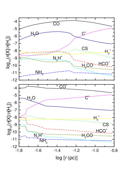
Figure 3: The log fractional abundances of various species as a function of the core radius at $t_{\rm coll}$ $=$ 1.36$\times$10⁵ yr (top) and 4.08$\times$10⁵ yr (bottom).

Having calculated the spatial distribution of the chemical abundances, we apply an appropriate radiative transfer model to be able to predict the observed line profiles. In this study we use smmol; a one-dimensional ALI code that solves multi-level non-LTE radiative transfer problems and which was described in RY01. Subsequent to that study, smmol has been benchmarked for accuracy (van Zadelhoff et al. 2002) and expanded to include a more comprehensive dataset of molecular collisional data. Defining an input continuum radiation field, the code calculates the total radiation field and the level populations, $n_{i}$, using a user-defined convergence criterion which we set to $\Delta n_{i}/n_{i}\leq 10^{-4}$. The emergent intensity distributions are then convolved with the telescope beam, so that the model directly predicts the spectral line profiles for a given source as observed with a given telescope. For the background radiation field we use the cosmic background continuum ($T_{\rm BB}$ = 2.72 K). We assume that the telescope beam can be approximated by a Gaussian, with a characteristic half power beam width (HPBW). In this paper we have concentrated on line profiles for the five lowest transitions of HCO⁺ and CS ($J$ $=$ 1$\to$0 to $J$ $=$ 5$\to$4), and the N₂H⁺ $J$ $=$ 1$\to$0 line (its hyperfine structure was, however, not considered; see Section 3.5). Data for HCO⁺ and N₂H⁺ – H₂ collisions were taken from Flower (1999) and for CS – H₂ collisions from Turner et al. (1992).

For a typical low mass star-forming region, the angular resolution of a single dish mm/sub-mm telescope is comparable to the angular size of the core. For our calculations we have adopted the physical parameters of the B335 core, as deduced from Zhou et al. (1993), but placing it at 500 pc (in the outskirts of the Gould Belt or at roughly the distance of the Orion molecular cloud). For the telescope beam we have used characteristics of a 45-m antenna corresponding to the Nobeyama class. We have used beam efficiency data from commonly used systems based on the Nobeyama 45-m, the IRAM 30-m, and the James Clerk Maxwell Telescope (JCMT) 15-m antennae and modelled these as a putative 45-m class telescope (putative in the sense that no 45-m dish exists that can fully sample the frequency range that covers all of the transitions that we have considered). The efficiencies across the frequency range thus correspond to Nobeyama ($<$145 GHz), IRAM (145 – 280 GHz) and the JCMT ($>$280 GHz). Beam efficiencies at line frequencies are interpolated values generated by the smmol code. For the range of frequencies that we considered the spatial coverage of the source is rather similar to that obtained with the JCMT 15-m antenna for a source distance of 250 pc (cf. the study by RY01). In Section 3.4 we comment on the sensitivity of the simulated line profiles to the adopted distance of the cloud. The beam was placed at the core’s centre in all cases and no spatial offsets were considered. The telescope/beam characteristics and utilized transitions are summarized in Table 2.

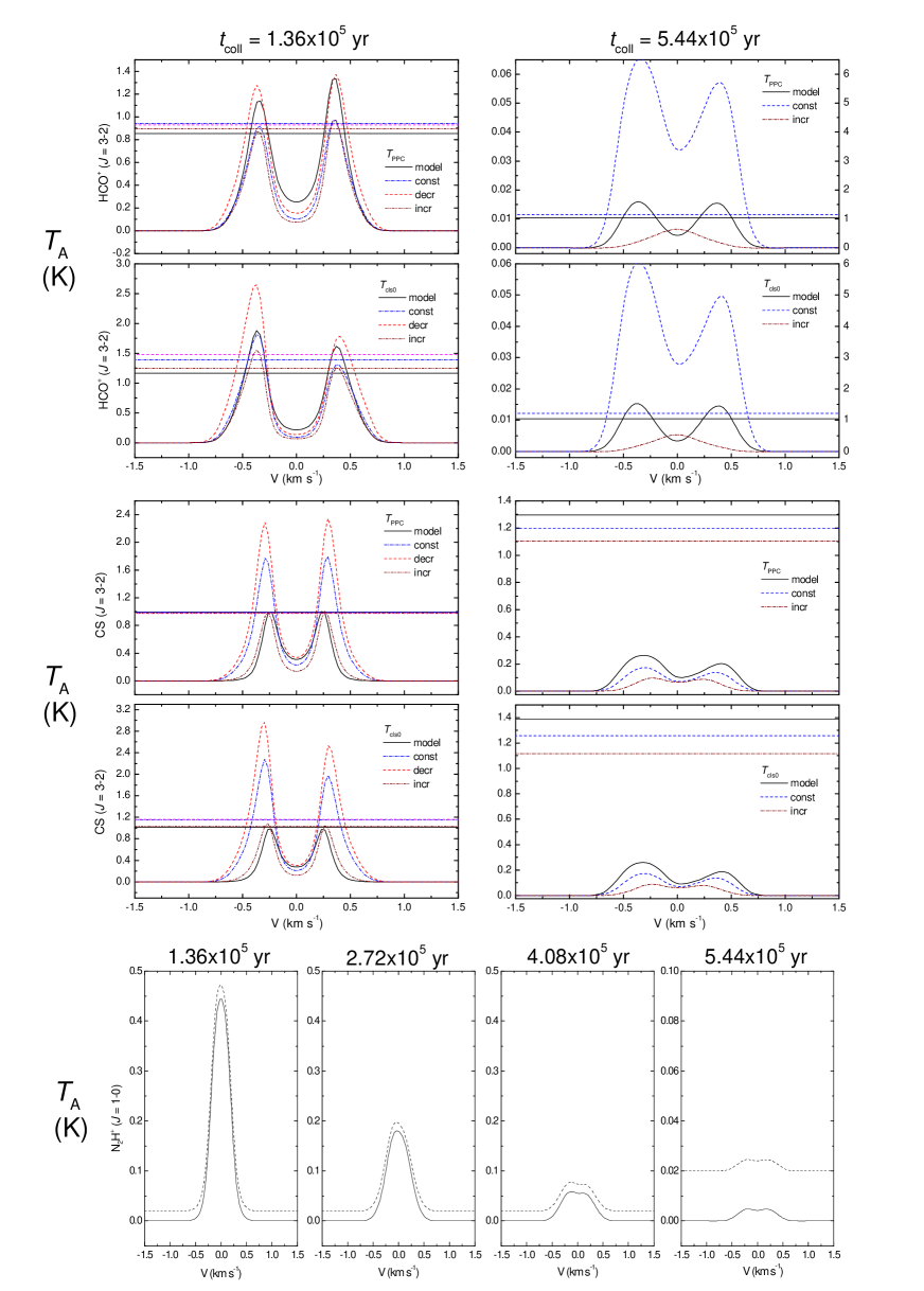
Figure 4: HCO⁺ ($J$ $=$ 3$\rightarrow$2) and CS ($J$ $=$ 3$\rightarrow$2) spectra for the $T_{\rm PPC}$ and $T_{\rm cls0}$ temperature profiles, at early and late collapse times $t_{\rm coll}$ $=$ 1.36$\times$10⁵ and 5.44$\times$10⁵ yr, respectively. The various profiles correspond to the ‘model’, ‘constant’, ‘decreasing’, and ‘increasing’ abundance distributions discussed in the text; the horizontal lines denote the respective blue/red asymmetry ratio (see Table A1; read off the right-hand axis for the two top-right HCO⁺ panels). The bottom four panels show the evolution of simulated N₂H⁺ ($J$ $=$ 1$\rightarrow$0) profiles for the $T_{\rm PPC}$ and $T_{\rm cls0}$ profiles across all collapse times adopting ‘model’ abundances divided by a factor of nine (solid and dashed line respectively; for clarity the latter was scaled up in intensity by $+$0.02 K. See Section 3.5 for details).

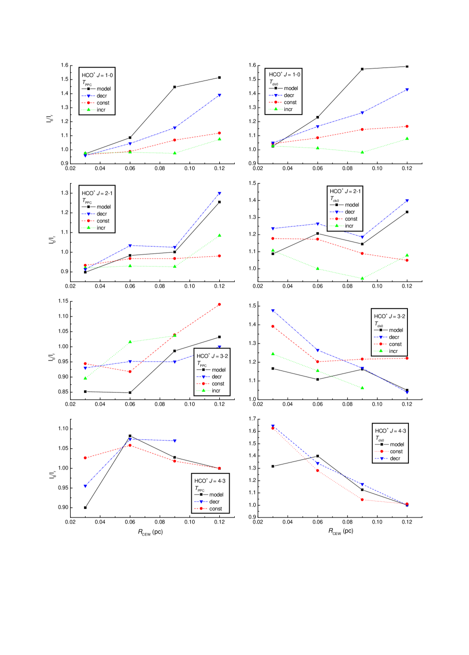
Figure 5: Evolution of the blue- to red-shifted line asymmetry for HCO⁺ ($J$ $=$ 1$\rightarrow$0, 2$\rightarrow$1, 3$\rightarrow$2, 4$\rightarrow$3) transitions for models with $T_{\rm PPC}$ and $T_{\rm cls0}$ temperature distributions.

3 Results and discussion

Raw results from the chemical models are given both in the form of a plot of the linear abundances as functions of position at a single time (Fig.  2) – which emphasizes the relative contributions of the different parts of the core to the line profiles – and a more conventional plot of the (logarithmic) abundances as functions of position at individual collapse times (Fig.  3). These represent the outputs obtained from the (independently integrated) Lagrangian grid of points.

Examples of the spectral line profiles for HCO⁺, CS and N₂H⁺ calculated using these abundances, the physical parameters obtained from the dynamical model and appropriate source/telescope parameters are shown in Fig.  4 (and also Fig.  12 – see below). For each of these line profiles the continuum (deriving from a combination of dust emission and the cosmic background radiation) has been subtracted so as to allow an easier comparison of the profiles. Line profiles are displayed for the first and last collapse periods for the HCO⁺ and CS $J$ = 3$\to$2 transitions.

The full set of results is given in numerical form in Table A1 of the Appendix. In constructing this table, and for the sake of brevity, we have reduced individual line profiles to the peak line intensities of the blue-shifted components ($I_{b}$) and the ratio of blue- to red-shifted component intensities ($I_{b}/I_{r}$). The tabulated intensities were determined by fitting Gaussians to the simulated line profiles as if they were observed spectra. We refer to the quantity $I_{b}/I_{r}$ as the line asymmetry ratio (or blue excess). This ratio is also marked by the horizontal lines in Fig.  4. Inspection of this figure allows the evaluation of the dependence of the line strength and asymmetry on the adopted abundance distributions in the core.

For almost all transitions and collapse periods considered in this study the peak line intensities, as well as the integrated fluxes, are the weakest for abundance distributions that increase outwards from the centre of the core. This can be explained in terms of a smaller optical depth and hence weaker emergent line intensity for regions of the core where the mass-averaged abundance of a molecular tracer is particularly low. For example, in the case of HCO⁺ at $t_{\rm coll}$ $=$ 1.36$\times$10⁵ yr this is true between $\sim$ 0.03 – 0.09 pc, and the line intensities corresponding to the ‘increasing’ abundance profile are typically weaker than for the other profiles. For CS the ‘model’ and ‘increasing’ abundance profiles show similar, radially increasing mass-averaged distributions out to $\sim$ 0.12 pc. The line intensities for these profiles are lower than for the constant and ‘decreasing’ profiles which are associated with larger mass-averaged abundances over the same region. Also, the difference in line intensities from the adoption of the ‘increasing’ as opposed to, for example, the ‘decreasing’ abundance profile is more pronounced for lines of higher critical density ($n_{\rm cr}$) and smaller HPBW as these are less efficiently excited at large core radii where the gas density is low.

In Figs.  5 and 7 we present plots of the line asymmetry ratio (using some of the values given in Table A1) for observationally interesting transitions of CS and HCO⁺ respectively, showing the temporal evolution of the line asymmetry ratio for models with a $T_{\rm PPC}$ and $T_{\rm cls0}$ temperature distribution. We can deduce several trends from these results and discuss them in the following subsections.

3.1 HCO⁺

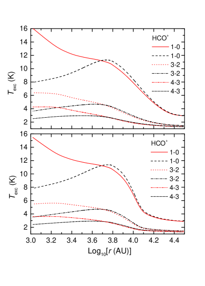
Figure 6: Excitation temperatures of HCO⁺ transitions corresponding to $t_{\rm coll}$ $=$ 1.36$\times$10⁵ yr: (Top) adopting the ‘decreasing’ abundance distribution; (Bottom) adopting the chemical model abundance distribution. Red curves are from the radiative transfer solution applicable to the $T_{\rm cls0}$ temperature profile and black curves are from the solution applicable to the $T_{\rm PPC}$ profile.

In our study we find that for both the $T_{\rm PPC}$ and $T_{\rm cls0}$ temperature distributions the line asymmetry ratio generally increases with time for the $J$ = 1–0 transition for the ‘model’ and ‘decreasing’ abundance distributions; it shows a very slight increase for a constant molecular abundance, while it remains mostly flat with the ‘increasing’ abundance distribution. In the latter case the line is almost symmetric, but the line does show a slight red asymmetry ($I_{\rm b}$/$I_{\rm r}$ $<$ 1) in models with a $T_{\rm PPC}$ temperature distribution: the symmetric profiles are due to the decreased line opacity resulting from the depressed molecular abundance towards the core’s centre. The slight red asymmetry is caused by a positive outward gradient of the line excitation temperature ($T_{\rm exc}$) given the $T_{\rm PPC}$ profile in the inner core. The blue asymmetry shows a rather stronger sensitivity on the abundance distribution for the 1–0 than for the 2–1 transition, especially at later times (Fig.  5).

The 2–1 line overall shows similar behaviours to that of the 1–0 line with rising asymmetry ratios at later times (except for a constant and ‘increasing’ abundance in the $T_{\rm cls0}$ case): the asymmetry ratios however are generally lower and this is caused by the smaller HPBW of this transition which covers about half the collapsing area of the cloud during each collapse period (relative to the 1–0 line), and the higher critical density of this line compared to the 1–0 transition (1.1$\times$10⁶ vs. 1.6$\times$10⁵ cm^-3). For the $T_{\rm cls0}$ temperature profile the asymmetry ratios of the 2–1, 3–2 and 4–3 lines initially (at 1.36 $\times$ 10⁵ yr) attain higher values than that of the 1–0 line. This is due to the smaller HPBWs of these lines which during that time respectively cover the central 38, 25, and 19 per cent of the infalling region thus sampling the warmest, dense inner regions of the cloud.

In Fig.  6 we show an example of the radiative transfer solution for the excitation temperature of representative HCO⁺ lines for both our adopted temperature profiles and for two different abundance distributions. For a given temperature profile the $T_{\rm exc}$ variations per line across the cloud appear similar, but the temperatures are all slightly higher in the top compared to the bottom panel along points in the cloud where the ‘decreasing’ abundance distribution results in a larger concentration of HCO⁺ than the ‘model’ abundance distribution. The opposing trends caused by the two different kinetic temperature profiles (Fig.  1) are especially evident towards the centre of the cloud. When adopting the $T_{\rm PPC}$ profile the $T_{\rm exc}$ of the lines shows a positive outward gradient in the inner cloud which results in red asymmetry ratios in the early collapse stages (Fig.  5). For the same temperature profile, the lines attain blue asymmetry ratios during the late collapse stages as the expanding CEW encounters a negative $T_{\rm exc}$ outward gradient (for log($r$) $\gtrsim$ 3.8): the 1–0 and 2–1 lines then reach slightly higher $I_{\rm b}$/$I_{\rm r}$ ratios than the 3–2 and 4–3 lines and this must be caused by the better sampling (larger HPBW) of the infalling region, combined with an increased line opacity for the former diagnostics (especially when the ‘model’ and ‘decreasing’ abundance distributions are adopted).

For the $T_{\rm cls0}$ temperature profile, the 3–2 and 4–3 lines initially show blue asymmetries ($I_{\rm b}$/$I_{\rm r}$ $>$ 1) with a spread depending on the adopted abundance distribution. This affects differently the line opacity in each case, but as the collapse progresses the line profiles become more symmetric: due to the central placement of the beams these high critical density lines (3.4$\times$10⁶ and 9.1$\times$10⁶ cm^-3respectively) cover at each successive collapse period a decreasing fraction of the infalling gas volume whose density steadily falls. At $t_{\rm coll}$ $=$ 5.44 $\times$ 10⁵ yr only 6 and 5 per cent of the infalling region is respectively sampled by the 3–2 and 4–3 lines compared to 19 per cent for the 1–0 line, and the central density has fallen below 5$\times$10⁴ cm^-3.

The $J$ $=$ 5–4 line is very weak for both adopted temperature profiles (due to the high critical density for the transition): it shows no central self-absorption in the $T_{\rm PPC}$ case, while it shows strong blue asymmetry at early times in the $T_{\rm cls0}$ case, becoming symmetric later on (Table A1).

3.2 CS

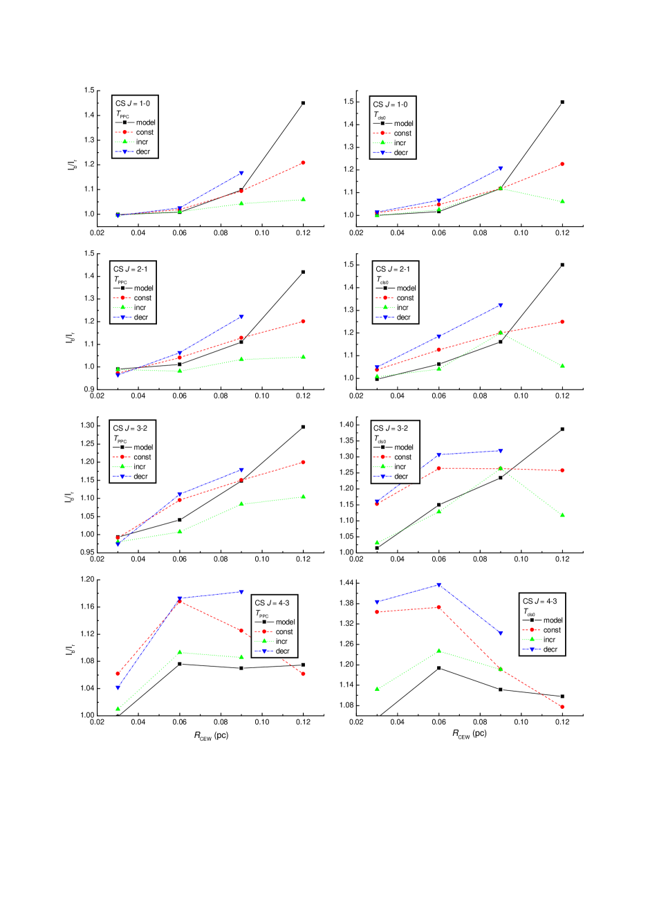
Figure 7: Evolution of the blue- to red-shifted line asymmetry for CS ($J$ $=$ 1$\rightarrow$0, 2$\rightarrow$1, 3$\rightarrow$2, 4$\rightarrow$3) transitions for models with $T_{\rm PPC}$ and $T_{\rm cls0}$ temperature distributions.

The $J$ $=$ 1–0, 2–1 and 3–2 transitions consistently show blue asymmetric profiles whose asymmetry increases at later times with both $T_{\rm PPC}$ and $T_{\rm cls0}$ temperature distributions, without a strong sensitivity on the adopted abundance for the species (Fig.  7). The only line that shows an opposite trend is the 4–3 transition which shows a blue asymmetry at early times (most clearly in the models with a $T_{\rm cls0}$ temperature profile), which becomes less prominent at later times. It is also strongly dependent on the adopted abundance distribution. This is also true for the 5–4 transition; this is always a very weak line. Compared to HCO⁺, the difference between the line asymmetry resulting from the adoption of different kinetic temperature profiles is not so pronounced, although for the $T_{\rm cls0}$ models slightly higher blue asymmetries are obtained. How can the different behaviour of CS compared to HCO⁺ be explained? A plot of $T_{\rm exc}$ for CS transitions reveals a broadly similar picture to Fig.  6 and the contrasting trends corresponding to the $T_{\rm PPC}$ and $T_{\rm cls0}$ cases remain. The outward gradient in the $T_{\rm exc}$ of all analyzed lines when adopting a $T_{\rm PPC}$ profile is however only slightly positive in contrast to the case of HCO⁺. Furthermore, all the CS lines have larger HPBWs than the corresponding HCO⁺ transitions with our 45-m antenna set-up. As a consequence, when adopting the $T_{\rm PPC}$ profile, the transitions plotted in Fig.  7 are all initially (at 1.36 $\times$ 10⁵ yr) approximately symmetric, in contrast to the HCO⁺ case where slightly negative asymmetry ratios are obtained. At later times as the beam footprint starts sampling infalling regions where the $T_{\rm exc}$ of the lines through the cloud becomes centrally peaked, the $I_{\rm b}$/$I_{\rm r}$ ratios typically increase. The high $n_{\rm cr}$ lines 4–3 and 5–4, which incidentally also have the smallest HPBWs, do not follow this trend at late collapse times because by then the core density is low and the lines are not sufficiently opaque compared to the lower $J$ transitions.

The 5–4 line becomes very weak after the first collapse period (Table A1) as it has a high critical density (9 $\times$ 10⁶ cm^-3) and cannot be efficiently excited in the decreasing density of the infalling envelope at later times. As CS is depleted in the chemical model in the inner core, the line appears optically thick and self-absorbed only for the constant and decreasing abundance distributions with a blue asymmetry that decreases rapidly after the first collapse age (as in HCO⁺ 4–3); again $T_{\rm cls0}$ models show higher blue asymmetry ratios than $T_{\rm PPC}$ models.

3.3 Chronometers of inside-out collapse?

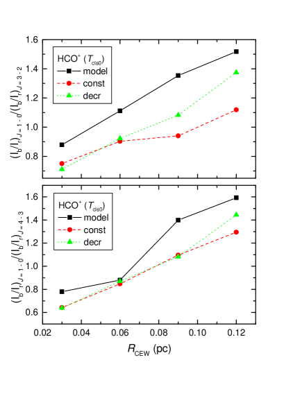
Figure 8: Evolution of the relative blue excess (the ratio of the respective line asymmetries) as function of the outer collapse expansion wave radius for HCO⁺, in a $T_{\rm cls0}$ model, for the ‘model’, ‘constant’, and ‘decreasing’ abundance distributions in the core: (Top) $J$ $=$ 1$\rightarrow$0 vs. 3$\rightarrow$2; (Bottom): $J$ $=$ 1$\rightarrow$0 vs. 4$\rightarrow$3 transitions. See also Table A1.

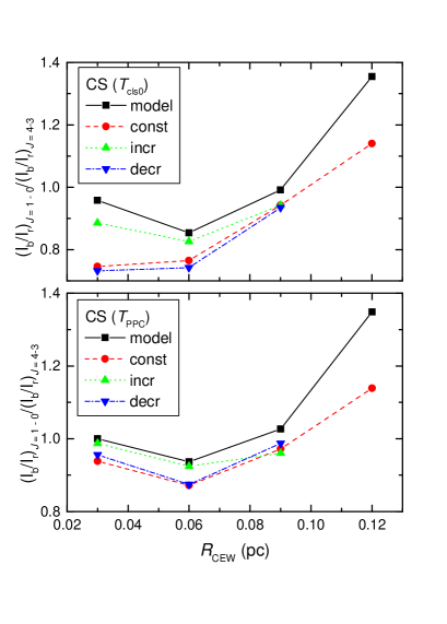
Figure 9: As in Fig.  8 but for CS $J$ $=$ 1$\rightarrow$0 vs. 4$\rightarrow$3 transitions: (Top) model core with a $T_{\rm cls0}$ temperature profile; (Bottom) model core with a $T_{\rm PPC}$ profile.

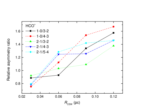
Figure 10: As in Fig.  8 but for the relative asymmetry ratios of the HCO⁺ lines noted in the key. The simulation is for a 15-m antenna for a core with a fixed $T_{\rm cls0}$ temperature profile and a ‘model’ HCO⁺ abundance distribution at a distance of 250 pc.

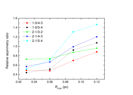
Figure 11: As in Fig.  8 but for the relative asymmetry ratios of the HCO⁺ lines noted in the key. The simulation is for a 45-m antenna for a core with a fixed $T_{\rm cls0}$ temperature profile and a constant HCO⁺ abundance distribution at a distance of 500 pc.

Studying the above results, we see that the HCO⁺ $J$ $=$ 3–2, 4–3, and 5–4 transitions follow an inverse trend in the temporal evolution of their blue asymmetry compared to the 1–0 transition. To help visualize these effects we plot in Fig.  8 the time evolution of the relative blue excess;

$$\mathcal{E}=\frac{(I_{b}/I_{r})_{1\to 0}}{(I_{b}/I_{r})_{4\to 3}},~{}\frac{(I_{b}/I_{r})_{1\to 0}}{(I_{b}/I_{r})_{3\to 2}}.$$

Results are shown for models with a $T_{\rm cls0}$ temperature profile where effects are most noticeable. Similarly, in Fig.  9 we plot the evolution of the relative blue excess, $\mathcal{E}$, of the CS $J$ $=$ 1–0 vs. the 4–3 transition (for models with $T_{\rm PPC}$ and $T_{\rm cls0}$ distributions). It can be seen that the $\mathcal{E}$ corresponding to these transitions depends on the dynamical age, and models with different abundance distributions follow the same general trend. A similar dependence is the one emerging from a comparison of the contrasting evolution of the HCO⁺ 4–3 vs. the CS 3–2 line (compare Figs.  5 and 7, for a core with a $T_{\rm cls0}$ temperature profile and a ‘model’ abundance distribution).

These behaviours are mostly due to the varying spatial sampling of parts of the core at various infall times by the different line frequencies employed, given the adopted 45-m antenna and the centrally placed beams. For instance, the HCO⁺ $J$ $=$ 1–0 line samples 76 per cent of the infall region at $t_{\rm coll}$ $=$ 2.72$\times$10⁵ yr, when the 3–2 and 4–3 transitions sample 25 and 19 per cent of its angular size respectively (using the parameters in Tables 1 and 2). In trials where the 3–2 and 4–3 transitions were modelled with a beam size that matched that of the 1–0 line, i.e. when employing a 11–15-m size antenna for the former lines and a 45-m antenna for the latter line, the evolution of the asymmetry for all these lines was roughly similar, and the trends in Fig.  8 virtually disappeared. The same case can be made for the CS trends of Fig.  9.

In order to test whether these results are the product of a particular modelling configuration, in Fig.  10 we plot the relative line asymmetry, $\mathcal{E}$, of HCO⁺ transitions modelled for a 15-m antenna (JCMT equivalent) and for a source distance of 250 pc. This results in approximately the same spatial coverage of the core by the various transitions as when the standard values of Table 2 are used. The ‘model’ HCO⁺ abundance distribution and the $T_{\rm cls0}$ temperature profile were adopted. The dependencies on the collapse period noted above hold in this case too. This shows that as long as the spatial coverage of the core remains approximately the same, the choice of modelling configuration does not significantly affect the trends of Fig.  8.

In order to further check whether these trends might still be valid for a much denser core model, we performed a simulation arbitrarily increasing the density across the core twenty-fold, up to a peak density of 3.6$\times$10⁶ cm^-3 at the onset of infall. This value is near the top of the range of densities inferred for a sample of protostellar cores in the Lynds clouds (Visser et al. 2002) and in Perseus (Motte & André 2001); although obviously unphysical in the context of the inside-out collapse model, this simulation serves to highlight the sensitivity to density. The relative line asymmetry ratios for a set of HCO⁺ transitions were obtained after evolving the cloud through the same collapse periods as for our standard 45-m antenna models (control parameters of Table 2). The results are plotted in Fig.  11 and show that the dependencies identified above are still valid.

Clearly, the trends in Figs.  8–11 imply that the behaviour of the relative blue excess of certain molecular transitions (observed with a given antenna) can be considered as a collapse chronometer in the formal context of the Shu model. We have therefore shown that in idealized spherically-symmetric cores which possess inward only motions, line measurements coupled to detailed models would in theory be able to constrain the evolutionary state of the (assumed inside-out) collapse. A number of caveats however must accompany this statement.

Firstly, the question of timescales. Observationally, the lifetime of submillimetre-detected, pre-stellar cores has been estimated from the statistics of detections of sources and approximate ages of 0.3 Myr have been established from an ensemble of various star-forming regions (Kirk et al. 2005). Based on estimates of the lifetime of Class I sources, and using statistical methods, a reference value for starless cores (PPCs) is $\sim$ 0.6 Myr (Kirk et al. 2007). In Perseus the lifetime of submm-detected starless cores was also estimated to be $\sim$ 0.4 Myr (Hatchell et al. 2007). The lifetime of Class 0 sources, which are potential manifestations of the inside-out collapse paradigm, has been revisited: whereas it was previously estimated that it may be one order of magnitude smaller than that of Class I sources, and of the order of 10⁴ yr (e.g. Ward-Thompson 1996), it is now thought that the relative Class 0/I phase lifetimes are similar (in the Perseus and Lynds dark clouds at least, and assuming a constant star formation rate), and of the order of a few $\times$ 10⁵ yr (Visser et al. 2002; Hatchell et al. 2007). The infall timescales we considered fall in this range. Moreover, the boundary between the Class 0/I phases in terms of observed evolutionary indicators is still elusive (Hatchell et al. 2007). We thus deem that, for the purposes of this work, the choice of timescales for our collapsing core analogue is not without due justification.

Another caveat involves the temperature profiles we have adopted in our models and which remain constant throughout the collapse phase. In realistic situations one would expect some overall heating to ensue at later times as mass accretes onto a central protostar. In order to get an idea of how this change in temperature might affect the line asymmetry, we run a model adopting a radial temperature profile, $T$($r$) $=$ 20($r$/1000 au)^0.36 K, corresponding to a source of $\sim$ 15 L_⊙ (taken from Ward-Thompson & Buckley 2001). Our typical Class 0 temperature profile (Fig.  1) is from the best-fit spectral energy distribution of B335 for a luminosity of $\sim$ 3 L_⊙ (Shirley et al. 2002) and so, in an approximate way, the above $T$($r$) should represent a considerable ‘evolution’ towards the Class I boundary. We find that for a constant HCO⁺ fractional abundance of 10^-8 the asymmetry ratio of HCO⁺ $J$ $=$ 1–0 rises more steeply than the one shown in Fig.  5 (top-right panel) corresponding to a model with a $T_{\rm cls0}$ temperature profile. If we were to assume that heating takes place after the second collapse period then the rise of the line asymmetry would be even more pronounced. The blue excess of the 4–3 line decreases linearly with collapse period, similarly to the model with a $T_{\rm cls0}$ profile, but attains slightly higher values throughout. We therefore conclude that the trend shown in Fig.  8 (bottom) would be little affected with this change of temperature law. Moreover, the line asymmetry of the 5–4 line is negligibly affected, and the 1–0/5–4 relative asymmetry ratio shows a dependence with dynamical age similar to those of Fig.  8 as well.

Finally, a stronger caveat involves the possible generic applicability of the identified ‘chronometers’ in studies of realistic infall candidates. As noted in Section 1, unfortunately, protostellar cores do not universally adhere to the inside-out paradigm of collapse. Observed non-zero velocities at large radii and/or small infall velocities at small radii, deviations from spherical symmetry, outflows, and rotation, are all likely to affect the line asymmetry of tracer species in ways that would be particular to each source. So would observational uncertainties, such as beam pointing inaccuracies. However, the identified trends are valid in the strict context of the inside-out collapse model and give us valuable insight into the ways the line asymmetry evolves and into the main factors that drive it.

In the next paragraph we examine the line profile sensitivity to the distance from the source.

3.4 Sensitivity to distance

Figure 12: Illustration of the dependence of the simulated line profile on the assumed distance to the a source with a $T_{\rm PPC}$ or $T_{\rm cls0}$ temperature distribution. Spectra from a 45-m antenna are plotted for distances of 50 pc (dotted lines), 250 pc (dashed lines) and 500 pc (solid lines).

The sensitivity of the line asymmetry ratio to source distance is a complex issue. For our nominal 45-m antenna the blue/red asymmetry of the HCO⁺ $J$ $=$ 1–0 transition increases by 22 per cent when the distance is decreased from 500 to 50 pc, whereas that of the $J$ $=$ 3–2 and 4–3 transitions decrease by $\sim$ 12 and 29 per cent respectively (for models with a $T_{\rm cls0}$ temperature profile). A possible explanation for these trends may be that the low $n_{\rm cr}$ 1–0 line samples better the denser infall region of the core at smaller distances than farther away, whereas the opposite is true for the higher $n_{\rm cr}$ 3–2, 4–3 lines which at small distances sample a very small fraction of the infall region (less than five per cent of the region within the 0.03 pc radius of the collapse expansion wave). A similar variation in absolute values is seen when adopting a 15-m antenna, but in that case the asymmetry ratio of the 3–2 and 4–3 transitions is larger at 250 pc.

An intrinsic property of the inside-out model seems to be that for whatever the distance to a source of given density, a set of transitions can be found whose optimum combination of HPBW (on a putative antenna), molecular tracer abundance, and line $n_{\rm cr}$, would allow them to act as collapse chronometers.

In Fig.  12 we plot the HCO⁺ 1–0 and 3–2 spectra of a core for a number of assumed distances, whilst keeping the beam size fixed (45-m antenna). They are for a model with $R_{\rm CEW}$ $=$ 0.03 pc and a constant molecular abundance. The peak line temperatures for models with a $T_{\rm cls0}$ temperature distribution decrease linearly with distance (apart from the 1–0 line whose peak temperature shows a faster decrease). This is due to the fact that at near distances the beam predominantly samples a denser portion of the core than at larger distances where a bigger volume of gas is sampled. Also, at near distances the peak centroids are found at higher velocities as the beam samples a faster moving gas flow at the core’s centre; a similar result was reported by Ward-Thompson and Buckley (2001). The same comments apply in the case of a core with a $T_{\rm PPC}$ temperature distribution.

We conclude that distance uncertainties for a given core are likely to affect significantly the simulated line asymmetry ratios as these depend critically on the coupling between the HPBW of the transition probe and the size of the infall region.

3.5 N₂H⁺

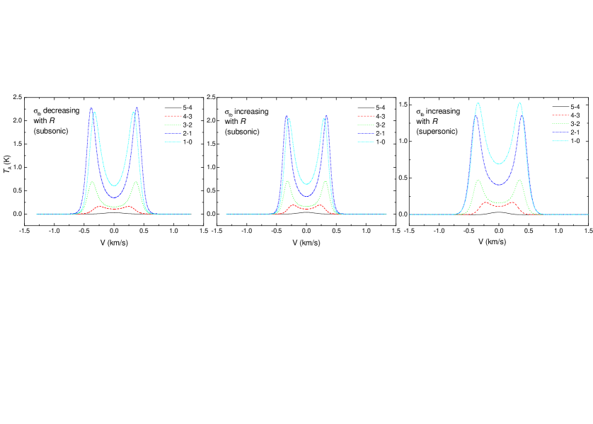
Figure 13: Illustration of the dependence of the simulated HCO⁺ line spectra of a static core on the assumed level of internal turbulence – the $T_{\rm cls0}$ temperature profile was adopted with a molecular abundance distribution as that shown in Fig.  2 (‘model’); see text for details.

The $J$ $=$ 1–0 transition of diazenilium has been modelled using only the molecular abundance from the chemical code as input to the RT code. The mean fractional abundance of N₂H⁺ in the chemical model displays a range of $\sim$ 1$\times$10^-10 to 9$\times$10^-10 in the timescales we considered; this is in very good agreement to the range found for a large sample of PPCs in the Perseus molecular cloud (Kirk, Johnstone, & Tafalla 2007). We have not attempted to model the N₂H⁺ hyperfine structure (see Pagani et al. 2007). In order to make our results more readily comparable to observations we have thus divided the molecular abundance corresponding to each collapse period by a factor of nine; this would approximately reproduce the flux of the isolated ‘blue’ hyperfine component $FF^{\prime}$ $=$ 01–12 (assuming that the hyperfine levels are populated in proportion to their statistical weights). This is usually better suited for analysis of infall candidates as it is mostly optically thin (Caselli et al. 1995; Mardones et al. 1997), and the other components can suffer from overlap which occurs due to the large intrinsic linewidths in dense cores resulting from non-thermal motions and opacity broadening. The line is extensively used in studies of star-forming cores as the tracer whose largely single-peaked nature argues against interpretations other than infall when trying to explain the blue asymmetry exhibited by other tracers.

A graph of the evolution of the transition during the collapse of the core analogue is shown in Fig.  4 (bottom). The line appears single peaked and optically thin for both the $T_{\rm PPC}$ and $T_{\rm cls0}$ temperature profiles, but becomes double peaked during the last two collapse periods when its peak intensity has dropped to about 10 and 2 per cent of its initial value. As the line is still optically thin in the two right panels of Fig.  4 (bottom) the double peak is not produced by self-absorption but instead it directly traces the infall velocity structure of the core. A comparison of the model spectra with the PPC observations presented by Lee et al. (1999) shows very good agreement in terms of peak intensity and line width with the range detected in their sample for the isolated component. At $t_{\rm coll}$ $=$ 1.36$\times$10⁵ yr the line characteristics resemble those of L183B, while at 4.08$\times$10⁵ yr the line looks very much like the one present in L492 (cf. fig.  5 in Lee et al.). In the context of inside-out collapse, the suitability of this line in the role of the optically thin tracer of infall (except perhaps in advanced stages) is re-affirmed by this work.

3.6 Microturbulence

In this paragraph we comment on the effects of varying levels of internal turbulence on the simulated spectra of a static core with a $T_{\rm cls0}$ temperature profile. By setting the infall velocity to zero in these models the effects of varying the turbulence are more readily observed. Ward-Thompson, Hartmann and Nutter (2005) have shown how increased levels of constant turbulent velocity dispersion, $\sigma_{\rm tb}$, throughout an infalling source lead to increased velocity separation of the line peaks. They reported peak velocity differences (i.e. separation of the blue/red peaks) of order $\Delta V$ $\sim$ 1–2 km s^-1 when the turbulent velocity varied between 1/3.5 and 1.14 times the adopted sound speed, $\alpha_{\rm eff}$, in a collapsing cloud.

We have investigated plausible monotonic variations of $\sigma_{\rm tb}$, increasing or decreasing with distance from the static core’s centre. We found that when $\sigma_{\rm tb}$ decreases outwards from subsonic values of 1.5$\sigma_{\rm NT}$ to $\sigma_{\rm NT}$ at the outer core radius (where $\sigma_{\rm NT}$ $\approx$ 0.145 km s^-1 is our nominal turbulent velocity dispersion), this produces a peak velocity separation of 0.7 and 0.8 km s^-1 for the HCO⁺ $J$ $=$ 1–0 and 2–1 transitions respectively (Fig.  13). When $\sigma_{\rm tb}$ instead increased with radius by the same amount (remaining subsonic), the peak velocity separation of the $J$ $=$ 1–0, 2–1, and 3–2 lines was $\sim$ 15 per cent smaller, while that of the 4–3 line changed by less than 10 per cent. Higher $J$ lines were not self-absorbed and the full width at half maximum of the 5–4 line was 20 per cent larger in the ‘decreasing’ compared to the ‘increasing’ $\sigma_{\rm tb}$ case (for the same radiant line flux). The differences in the velocity separation of the line peaks that we found in these two simple examples are similar in magnitude to what one obtains if the optical depth of the lines are increased by a factor of $\sim$2 as Ward-Thompson, Hartmann and Nutter report. However, this may be the case only for small $\sigma_{\rm tb}$ variations, such as these in our example; Ward-Thompson and Buckley (2001) found that various power-law relations between $\sigma_{\rm tb}$ and the gas density, encompassing a wider range than we have considered, have a more substantial effect on the peak velocity separation for the HCO⁺ $J$ $=$ 4–3 and CS $J$ $=$ 5–4 lines.

We also note that uncertainties in the distance to the source can mimic the effects on the peak velocity separation produced by the range of $\sigma_{\rm tb}$ we have explored. The distance uncertainties to protostellar cores, however, do not usually exceed a factor of two and so the effects are probably separable. If one includes an analysis of optically thin lines as well, then the potential degeneracy between distance and turbulence effects can be avoided.

Supersonic turbulence in the outer parts of pre-stellar cores has been associated with outflows or with generic turbulence permeating from the parent molecular clouds. We have thus investigated an outward increase of turbulence to supersonic values at the edge of the core ($\sim$ 2$\alpha_{\rm eff}$), encompassing a factor of three variation from the inner to the outer radius. This is similar to that observed in the Class 0 source NGC 1333-IRAS 4A (Belloche, Hennebelle, & André 2006). The velocity separation of the peaks in this case (Fig.  13 right) is similar to what is obtained with a radially decreasing subsonic $\sigma_{\rm tb}$. This situation however is clearly distinguishable from the subsonic models as the total flux in the self-absorbed lines ($J_{\rm up}$ $\leqslant$ 4) is lower. In the supersonic turbulence case, the optical depth of the lines in the centre of the core relative to the outer regions is larger as increased levels of turbulence in the outer core result in lower optical depths (as the optical depth is inversely proportional to the line width; see also Ward-Thompson and Buckley 2001); hence the emission in the self-absorption trough which is more weighted towards the inner core, is enhanced relative to that in the peaks.

4 conclusions

Using a coupled chemodynamical and RT model we have conducted an exploratory study of the evolution of the spectral line characteristics (intensities and asymmetries) of molecular species such as HCO⁺, CS, and N₂H⁺, which are frequently used as tracers of collapse in star-formation studies. We have investigated the sensitivity of the line diagnostics to several chemical abundance distributions and to the thermal structure of a low-mass core analogue undergoing inside-out collapse.

Table 3: Comparison of the mean ‘blue-excess’ $I_{\rm b}$/$I_{\rm r}$ for models with a $T_{\rm PPC}$ and $T_{\rm cls0}$ temperature distribution (from all abundance distributions and transitions) at early (‘1’: $t_{\rm coll}$ $=$ 1.36$\times$10⁵ yr) and late (‘2’: $t_{\rm coll}$ $=$ 5.44$\times$10⁵ yr) collapse periods.

HCO+
$T_{\rm PPC}$	$T_{\rm cls0}$	Ratio
1.   0.936$\pm$0.043	1.334$\pm$0.527	1.425$\pm$0.441
2.   1.221$\pm$0.308	1.159$\pm$0.184	0.949$\pm$0.411
CS
1.   1.012$\pm$0.050	1.149$\pm$0.051	1.135$\pm$0.094
2.   1.188$\pm$0.163	1.225$\pm$0.190	1.031$\pm$0.292

In Table 3 we compare the mean line asymmetry ratio of models with $T_{\rm PPC}$ and $T_{\rm cls0}$ temperature profiles (respectively applicable to starless cores and cores with a warm central region), for the five lowest transitions of HCO⁺ and CS, at early and late collapse times (the errors are 1$\sigma$ standard deviations). This rather crude comparison smoothes out the effects of different abundance distributions, but helps us to see that at early times HCO⁺ is generally a more sensitive probe of collapse than CS (at least in $T_{\rm cls0}$ models), mainly because its higher excitation transitions resolve the infall region better than the respective CS lines. At later times the situation is mildly reversed (for $T_{\rm cls0}$), mainly because CS 3–2 and 4–3 trace relatively better the low density infalling envelope. For both species the mean asymmetry is stronger in $T_{\rm cls0}$ models than in $T_{\rm PPC}$ models at the onset of infall, but this difference almost disappears later on. Also, while for CS the line asymmetry increases on average from early to late times, the HCO⁺ asymmetry for the $T_{\rm cls0}$ models decreases on average in the same length of time.

When different abundance distributions are considered then the picture becomes more complicated. Figs.  4 and 7 show that if the molecular tracer’s abundance increases towards large core radii then the lines can appear symmetric even at advanced stages of infall. This is mostly evident in models with a $T_{\rm PPC}$ temperature profile which are not conducive to large blue excesses in general and for which red asymmetry ratios can be obtained. Conversely, a molecular abundance which declines with radius can result in high values of blue excess – this is particularly evident in the behaviour of some lines at early times. Finally, a consequence of the specific chemical model used in this study is that the existence of high HCO⁺/CS abundance ratios in the inner core contributes, at early collapse times, to a lower line asymmetry for CS than for HCO⁺ lines.

The main conclusions of this analysis of Shu-type infall are:

1. Overall, HCO⁺ is a somewhat better tracer of core collapse than CS, but this depends on the evolutionary state of the core, as there is a direct correspondence between the critical density of a particular transition and its ability to trace gas of given density and temperature (with a significant excitation temperature and optical depth). N₂H⁺ $J$ $=$ 1–0 is well suited as the optically thin ‘control’ line in infall studies (except perhaps in advanced evolutionary stages).

2. In the context of inside-out infall (in the absence of rotation) the relative blue asymmetry of certain transitions is a function of the dynamical age (for a given telescope), and acts as a ‘collapse chronometer’. This is mainly due to a combination of beam filling factors and line critical densities: a line of high critical density whose beamwidth efficiently resolves the infall region shows higher blue asymmetry at early collapse times than at later times when the gas density becomes too low; the opposite is true for a line of low critical density whose large beamwidth cannot adequately resolve the infall region at early times, but does so later on whilst remaining sufficiently opaque in the lower density conditions.

3. The line asymmetry ratio is dependent on the abundance distribution of the molecular tracer in the source. The dependence naturally becomes stronger when the line beamwidth resolves the infall region well. Detailed chemical models are therefore very important tools when attempting to interpret the observations.

4. Distance uncertainties of a factor of two or greater affect the line asymmetry ratio significantly.

5. Subsonic turbulence which monotonically decreases outwards from the core centre by a factor of 1.5 produces peak velocity separations in the HCO⁺ 1–0, 2–1 lines of the order of $\sim$1 km s^-1. This is comparable to the peak velocity separations caused by an uncertainty estimate in the distance of a factor of five. A turbulence which increases with radius by a factor of 1.5 has a smaller effect on the peak velocity separation. Turbulence which monotonically increases outwards to supersonic values, with a variation of a factor of three in the core, produces similar peak velocity separations to the subsonic decreasing case, but results in a much stronger self-absorption in the lines.

In the future we shall study the sensitivities of line profiles to the infall dynamics [$v(r)$, in both the collapse and pre-collapse phases] and the chemical and physical initial conditions. And although this work is of a general nature, the method of analysis and application can easily be adapted to model specific sources and instrumental configurations. Concerning the latter, the next development will be to generate a spectral line interpretation ‘atlas’ for use in the analysis of Herschel HIFI datasets.

Acknowledgments

This work was made possible through use of the HiPerSPACE supercomputer facility at UCL and has made use of the NASA ADS database. We thank an anonymous referee and D. Ward-Thompson for their critical and in depth review of this article. We also appreciate helpful comments from N. J. Evans. YGT acknowledges support from an STFC postdoctoral grant.

Appendix A Model peak line intensities and asymmetry ratios

Table 1: Temporal evolution of molecular line peak intensities ($I$) and respective ratios (the line asymmetry ratio) as measured from our simulated spectra: subscript ‘b’ denotes blue-shifted, ‘r’ denotes red-shifted. The adopted abundance profiles are discussed in Section 2.1. $T_{\rm PPC}$ and $T_{\rm cls0}$ are the temperature distributions shown in Fig.  1.

	$I_{\rm b}$	$I_{\rm b}$/$I_{\rm r}$	$I_{\rm b}$	$I_{\rm b}$/$I_{\rm r}$
	(K)		(K)
	$T_{\rm PPC}$		$T_{\rm cls0}$
$t_{\rm coll}$ $=$ 1.36$\times$105 yr	HCO+
	$n_{\rm mol}$($r$) $=$ ‘model’
$J$ $=$ 1$\rightarrow$0	2.619	0.972	2.620	1.025
2$\rightarrow$1	2.910	0.898	3.658	1.088
3$\rightarrow$2	1.136	0.852	1.881	1.166
4$\rightarrow$3	0.390	0.899	0.909	1.316
5$\rightarrow$4	–	–	0.122	1.369
	$n_{\rm mol}$($r$) $=$ ‘constant’
$J$ $=$ 1$\rightarrow$0	1.767	0.967	1.897	1.044
2$\rightarrow$1	2.234	0.933	3.151	1.178
3$\rightarrow$2	0.915	0.944	1.814	1.391
4$\rightarrow$3	0.259	1.027	0.901	1.625
5$\rightarrow$4	0.027	–	0.136	1.260
	$n_{\rm mol}$($r$) $=$ ‘increasing’
$J$ $=$ 1$\rightarrow$0	1.813	0.975	1.849	1.028
2$\rightarrow$1	2.130	0.920	2.852	1.107
3$\rightarrow$2	0.870	0.895	1.558	1.244
4$\rightarrow$3	0.012	–	0.721	1.487
5$\rightarrow$4	0.012	–	0.101	1.199
	$n_{\rm mol}$($r$) $=$ ‘decreasing’
$J$ $=$ 1$\rightarrow$0	2.282	0.959	2.443	1.050
2$\rightarrow$1	2.733	0.913	4.091	1.237
3$\rightarrow$2	1.278	0.930	2.639	1.476
4$\rightarrow$3	0.048	0.955	1.753	1.646
5$\rightarrow$4	0.049	–	0.321	1.734
	CS
	$n_{\rm mol}$($r$) $=$ ‘model’
$J$ $=$ 1$\rightarrow$0	1.509	0.999	1.418	0.999
2$\rightarrow$1	1.201	0.991	1.1541	0.996
3$\rightarrow$2	0.992	0.993	0.989	1.015
4$\rightarrow$3	0.290	0.999	0.300	1.043
5$\rightarrow$4	0.058	–	0.060	–
	$n_{\rm mol}$($r$) $=$ ‘constant’
$J$ $=$ 1$\rightarrow$0	1.470	0.996	1.435	1.011
2$\rightarrow$1	1.469	0.973	1.580	1.037
3$\rightarrow$2	1.777	0.991	2.280	1.153
4$\rightarrow$3	0.849	1.062	1.368	1.355
5$\rightarrow$4	0.159	1.108	0.377	1.590
	$n_{\rm mol}$($r$) $=$ ‘increasing’
$J$ $=$ 1$\rightarrow$0	1.276	0.997	1.220	0.999
2$\rightarrow$1	1.053	0.988	1.052	1.007
3$\rightarrow$2	0.993	0.980	1.078	1.031
4$\rightarrow$3	0.330	1.010	0.420	1.128
5$\rightarrow$4	0.068	–	0.088	–
	$n_{\rm mol}$($r$) $=$ ‘decreasing’
$J$ $=$ 1$\rightarrow$0	1.753	0.996	1.708	1.014
2$\rightarrow$1	1.809	0.964	1.968	1.051
3$\rightarrow$2	2.285	0.974	2.943	1.161
4$\rightarrow$3	1.253	1.042	2.051	1.385
5$\rightarrow$4	0.277	1.158	0.697	1.698
	N2H+
	$n_{\rm mol}$($r$) $=$ ‘model’
$J$ $=$ 1$\rightarrow$0	0.443	–	0.440	–

Table 1: –continued

	$I_{\rm b}$	$I_{\rm b}$/$I_{\rm r}$	$I_{\rm b}$	$I_{\rm b}$/$I_{\rm r}$
	(K)		(K)
	$T_{\rm PPC}$		$T_{\rm cls0}$
$t_{\rm coll}$ $=$ 2.72$\times$105 yr	HCO+
	$n_{\rm mol}$($r$) $=$ ‘model’
$J$ $=$ 1$\rightarrow$0	2.476	1.087	2.600	1.231
2$\rightarrow$1	2.394	0.984	2.857	1.207
3$\rightarrow$2	0.572	0.848	0.776	1.108
4$\rightarrow$3	0.120	1.082	0.184	1.399
5$\rightarrow$4	0.008	1.000	0.012	1.024
	$n_{\rm mol}$($r$) $=$ ‘constant’
$J$ $=$ 1$\rightarrow$0	1.718	0.988	1.789	1.086
2$\rightarrow$1	1.783	0.967	2.106	1.174
3$\rightarrow$2	0.371	0.917	0.513	1.202
4$\rightarrow$3	0.064	1.058	0.104	1.281
5$\rightarrow$4	–	–	–	–
	$n_{\rm mol}$($r$) $=$ ‘increasing’
$J$ $=$ 1$\rightarrow$0	1.039	0.982	1.013	1.011
2$\rightarrow$1	0.769	0.929	0.769	1.000
3$\rightarrow$2	0.115	1.016	0.115	1.154
4$\rightarrow$3	0.025	–	0.018	–
5$\rightarrow$4	0.002	–	–	–
	$n_{\rm mol}$($r$) $=$ ‘decreasing’
$J$ $=$ 1$\rightarrow$0	1.877	1.045	1.980	1.166
2$\rightarrow$1	1.935	1.034	2.360	1.264
3$\rightarrow$2	0.411	0.951	0.602	1.264
4$\rightarrow$3	0.073	1.074	0.129	1.341
5$\rightarrow$4	0.005	–	0.009	1.007
	CS
	$n_{\rm mol}$($r$) $=$ ‘model’
$J$ $=$ 1$\rightarrow$0	1.261	1.008	1.200	1.017
2$\rightarrow$1	0.881	1.011	0.878	1.063
3$\rightarrow$2	0.551	1.041	0.575	1.150
4$\rightarrow$3	0.116	1.076	0.126	1.190
5$\rightarrow$4	0.013	–	0.013	–
	$n_{\rm mol}$($r$) $=$ ‘constant’
$J$ $=$ 1$\rightarrow$0	1.264	1.019	1.235	1.048
2$\rightarrow$1	1.073	1.041	1.114	1.126
3$\rightarrow$2	0.835	1.095	0.945	1.264
4$\rightarrow$3	0.208	1.168	0.259	1.369
5$\rightarrow$4	0.022	–	0.030	1.064
	$n_{\rm mol}$($r$) $=$ ‘increasing’
$J$ $=$ 1$\rightarrow$0	1.254	1.010	1.208	1.025
2$\rightarrow$1	0.947	0.982	0.956	1.040
3$\rightarrow$2	0.679	1.008	0.721	1.128
4$\rightarrow$3	0.153	1.093	0.173	1.240
5$\rightarrow$4	0.019	–	0.018	–
	$n_{\rm mol}$($r$) $=$ ‘decreasing’
$J$ $=$ 1$\rightarrow$0	1.590	1.026	1.558	1.066
2$\rightarrow$1	1.502	1.063	1.597	1.186
3$\rightarrow$2	1.350	1.112	1.566	1.307
4$\rightarrow$3	0.392	1.173	0.509	1.436
5$\rightarrow$4	0.047	1.061	0.070	1.193
	N2H+
	$n_{\rm mol}$($r$) $=$ ‘model’
$J$ $=$ 1$\rightarrow$0	0.180	–	0.177	–

Table 1: –continued

	$I_{\rm b}$	$I_{\rm b}$/$I_{\rm r}$	$I_{\rm b}$	$I_{\rm b}$/$I_{\rm r}$
	(K)		(K)
	$T_{\rm PPC}$		$T_{\rm cls0}$
$t_{\rm coll}$ $=$ 4.08$\times$105 yr	HCO+
	$n_{\rm mol}$($r$) $=$ ‘model’
$J$ $=$ 1$\rightarrow$0	1.809	1.447	1.845	1.574
2$\rightarrow$1	1.336	1.001	1.457	1.145
3$\rightarrow$2	0.227	0.986	0.253	1.163
4$\rightarrow$3	0.038	1.028	0.041	1.125
5$\rightarrow$4	0.002	1.000	0.002	1.005
	$n_{\rm mol}$($r$) $=$ ‘constant’
$J$ $=$ 1$\rightarrow$0	1.363	1.070	1.360	1.144
2$\rightarrow$1	0.962	0.968	1.009	1.090
3$\rightarrow$2	0.140	1.039	0.151	1.217
4$\rightarrow$3	0.018	1.018	0.019	1.044
5$\rightarrow$4	–	–	–	–
	$n_{\rm mol}$($r$) $=$ ‘increasing’
$J$ $=$ 1$\rightarrow$0	0.957	0.976	0.902	0.981
2$\rightarrow$1	0.552	0.926	0.503	0.943
3$\rightarrow$2	0.064	1.037	0.053	1.062
4$\rightarrow$3	0.015	–	0.010	–
5$\rightarrow$4	0.001	–	$<$10-3	–
	$n_{\rm mol}$($r$) $=$ ‘decreasing’
$J$ $=$ 1$\rightarrow$0	1.927	1.158	1.957	1.265
2$\rightarrow$1	1.620	1.026	1.753	1.187
3$\rightarrow$2	0.270	0.951	0.310	1.169
4$\rightarrow$3	0.043	1.070	0.049	1.170
5$\rightarrow$4	0.003	1.001	$<$10-3	1.003
	CS
	$n_{\rm mol}$($r$) $=$ ‘model’
$J$ $=$ 1$\rightarrow$0	0.951	1.099	0.908	1.117
2$\rightarrow$1	0.561	1.109	0.546	1.160
3$\rightarrow$2	0.267	1.148	0.261	1.234
4$\rightarrow$3	0.042	1.070	0.039	1.127
5$\rightarrow$4	0.004	–	0.003	–
	$n_{\rm mol}$($r$) $=$ ‘constant’
$J$ $=$ 1$\rightarrow$0	1.039	1.094	1.005	1.118
2$\rightarrow$1	0.739	1.128	0.738	1.200
3$\rightarrow$2	0.408	1.151	0.418	1.263
4$\rightarrow$3	0.075	1.125	0.077	1.186
5$\rightarrow$4	0.006	1.010	0.006	1.017
	$n_{\rm mol}$($r$) $=$ ‘increasing’
$J$ $=$ 1$\rightarrow$0	0.950	1.043	1.005	1.118
2$\rightarrow$1	0.593	1.034	0.738	1.200
3$\rightarrow$2	0.298	1.084	0.418	1.263
4$\rightarrow$3	0.048	1.086	0.077	1.186
5$\rightarrow$4	0.005	–	0.006	1.017
	$n_{\rm mol}$($r$) $=$ ‘decreasing’
$J$ $=$ 1$\rightarrow$0	1.240	1.168	1.207	1.209
2$\rightarrow$1	0.983	1.223	0.995	1.323
3$\rightarrow$2	0.589	1.179	0.618	1.319
4$\rightarrow$3	0.123	1.182	0.131	1.293
5$\rightarrow$4	0.011	1.014	0.012	1.028
	N2H+
	$n_{\rm mol}$($r$) $=$ ‘model’
$J$ $=$ 1$\rightarrow$0	0.058	1.036	0.056	1.036

Table 1: –continued

	$I_{\rm b}$	$I_{\rm b}$/$I_{\rm r}$	$I_{\rm b}$	$I_{\rm b}$/$I_{\rm r}$
	(K)		(K)
	$T_{\rm PPC}$		$T_{\rm cls0}$
$t_{\rm coll}$ $=$ 5.44$\times$105 yr	HCO+
	$n_{\rm mol}$($r$) $=$ ‘model’
$J$ $=$ 1$\rightarrow$0	0.354	1.514	0.347	1.594
2$\rightarrow$1	0.149	1.255	0.148	1.332
3$\rightarrow$2	0.016	1.032	0.015	1.050
4$\rightarrow$3	0.002	0.999	0.002	1.001
5$\rightarrow$4	–	–	$<$10-3	–
	$n_{\rm mol}$($r$) $=$ ‘constant’
$J$ $=$ 1$\rightarrow$0	0.970	1.119	0.943	1.166
2$\rightarrow$1	0.510	0.981	0.498	1.050
3$\rightarrow$2	0.065	1.140	0.061	1.221
4$\rightarrow$3	0.008	1.010	0.006	1.010
5$\rightarrow$4	–	–	–	–
	$n_{\rm mol}$($r$) $=$ ‘increasing’
$J$ $=$ 1$\rightarrow$0	0.160	1.075	0.150	1.078
2$\rightarrow$1	0.050	1.084	0.045	1.089
3$\rightarrow$2	0.006	–	0.005	–
4$\rightarrow$3	0.001	–	$<$10-3	–
5$\rightarrow$4	–	–	$<$10-3	–
	CS
	$n_{\rm mol}$($r$) $=$ ‘model’
$J$ $=$ 1$\rightarrow$0	0.814	1.450	0.787	1.499
2$\rightarrow$1	0.551	1.418	0.543	1.500
3$\rightarrow$2	0.264	1.297	0.260	1.387
4$\rightarrow$3	0.045	1.075	0.043	1.107
5$\rightarrow$4	0.004	1.008	0.003	1.009
	$n_{\rm mol}$($r$) $=$ ‘constant’
$J$ $=$ 1$\rightarrow$0	0.718	1.209	0.688	1.226
2$\rightarrow$1	0.410	1.201	0.397	1.249
3$\rightarrow$2	0.181	1.199	0.173	1.258
4$\rightarrow$3	0.026	1.061	0.024	1.076
5$\rightarrow$4	0.002	1.007	0.002	1.009
	$n_{\rm mol}$($r$) $=$ ‘increasing’
$J$ $=$ 1$\rightarrow$0	0.591	1.059	0.564	1.060
2$\rightarrow$1	0.271	1.043	0.254	1.053
3$\rightarrow$2	0.098	1.104	0.088	1.117
4$\rightarrow$3	0.014	–	0.012	–
5$\rightarrow$4	0.001	–	0.001	–
	N2H+
	$n_{\rm mol}$($r$) $=$ ‘model’
$J$ $=$ 1$\rightarrow$0	0.005	1.001	0.005	1.003

References

- [Belloche et al.(2002)] Belloche, A., André, P., Despois, D., & Blinder, S. 2002, A&A, 393, 927
- [Belloche et al.(2006)] Belloche, A., Hennebelle, P., & André, P. 2006, A&A, 453, 145
- [Brooke et al.(2007)] Brooke, T. Y., et al. 2007, ApJ, 655, 364
- [Caselli et al.(1995)] Caselli, P., Myers, P. C., & Thaddeus, P. 1995, ApJL, 455, L77
- [Choi(2007)] Choi, M. 2007, PASJ, 59, L41
- [Choi et al.(1995)] Choi, M., Evans, N. J., II, Gregersen, E. M., & Wang, Y. 1995, ApJ, 448, 742
- [Danby et al.(1988)] Danby, G., Flower, D. R., Valiron, P., Schilke, P., & Walmsley, C. M. 1988, MNRAS, 235, 229
- [De Vries & Myers(2005)] De Vries, C. H., & Myers, P. C. 2005, ApJ, 620, 800
- [Evans(1999)] Evans, N. J., II 1999, ARA&A, 37, 311
- [Evans et al.(2001)] Evans, N. J., II, Rawlings, J. M. C., Shirley, Y. L., & Mundy, L. G. 2001, ApJ, 557, 193
- [Evans et al.(2005)] Evans, N. J., II, Lee, J.-E., Rawlings, J. M. C., & Choi, M. 2005, ApJ, 626, 919
- [Flower(1999)] Flower, D. R. 1999, MNRAS, 305, 651
- [Jørgensen et al.(2006)] Jørgensen, J. K., et al. 2006, ApJ, 645, 1246
- [Gregersen & Evans(2000)] Gregersen, E. M., & Evans, N. J., II 2000, ApJ, 538, 260
- [Gregersen et al.(2000)] Gregersen, E. M., Evans, N. J., II, Mardones, D., & Myers, P. C. 2000, ApJ, 533, 440
- [Hatchell et al.(2007)] Hatchell, J., Fuller, G. A., Richer, J. S., Harries, T. J., & Ladd, E. F. 2007, A&A, 468, 1009
- [Kirk et al.(2005)] Kirk, J. M., Ward-Thompson, D., & André, P. 2005, MNRAS, 360, 1506
- [Kirk et al.(2007)] Kirk, J. M., Ward-Thompson, D., & André, P. 2007, MNRAS, 375, 843
- [Kirk et al.(2007)] Kirk, H., Johnstone, D., & Tafalla, M. 2007, ApJ, 668, 1042
- [Lee et al.(1999)] Lee, C. W., Myers, P. C., & Tafalla, M. 1999, ApJ, 526, 788
- [Lee et al.(2007)] Lee, S. H., Park, Y.-S., Sohn, J., Lee, C. W., & Lee, H. M. 2007, ApJ, 660, 1326
- [Mardones et al.(1997)] Mardones, D., Myers, P. C., Tafalla, M., Wilner, D. J., Bachiller, R., & Garay, G. 1997, ApJ, 489, 719
- [Millar et al.(1997)] Millar, T. J., Farquhar, P. R. A., & Willacy, K. 1997, A&AS, 121, 139
- [Millar et al.(1991)] Millar, T. J., Bennett, A., Rawlings, J. M. C., Brown, P. D., & Charnley, S. B. 1991, A&AS, 87, 585
- [Motte & André(2001)] Motte, F., & André, P. 2001, A&A, 365, 440
- [Pagani et al.(2007)] Pagani, L., Bacmann, A., Cabrit, S., & Vastel, C. 2007, A&A, 467, 179
- [Pavlyuchenkov et al.(2006)] Pavlyuchenkov, Y., Wiebe, D., Launhardt, R., & Henning, T. 2006, ApJ, 645, 1212
- [Porras et al.(2007)] Porras, A., et al. 2007, ApJ, 656, 493
- [Rawlings et al.(1992)] Rawlings J.M.C., Hartquist T.W., Menten K.M., Williams D.A. 1992, MNRAS, 255, 471
- [Rawlings & Yates(2001)] Rawlings, J. M. C., & Yates, J. A. 2001, MNRAS, 326, 1423 (RY01)
- [Rawlings et al.(2002)] Rawlings, J. M. C., Hartquist, T. W., Williams, D. A., & Falle, S. A. E. G. 2002, A&A, 391, 681
- [Redman et al.(2004)] Redman, M. P., Keto, E., Rawlings, J. M. C., & Williams, D. A. 2004, MNRAS, 352, 1365
- [Roberts et al.(2007)] Roberts, J. F., Rawlings, J. M. C., Viti, S., & Williams, D. A. 2007, MNRAS, 382, 733
- [Shirley et al.(2002)] Shirley, Y. L., Evans, N. J., II, & Rawlings, J. M. C. 2002, ApJ, 575, 337
- [] Shu F. H., 1977, ApJ, 214, 488
- [Shu et al.(1987)] Shu, F. H., Adams, F. C., & Lizano, S. 1987, ARA&A, 25, 23
- [Sohn et al.(2007)] Sohn, J., Lee, C. W., Park, Y.-S., Lee, H. M., Myers, P. C., & Lee, Y. 2007, ApJ, 664, 928
- [Swift et al.(2006)] Swift, J. J., Welch, W. J., Di Francesco, J., & Stojimirović, I. 2006, ApJ, 637, 392
- [Tafalla et al.(1998)] Tafalla, M., Mardones, D., Myers, P. C., Caselli, P., Bachiller, R., & Benson, P. J. 1998, ApJ, 504, 900
- [van Zadelhoff et al.(2002)] van Zadelhoff, G.-J., et al. 2002, A&A, 395, 373
- [Visser et al.(2002)] Visser, A. E., Richer, J. S., & Chandler, C. J. 2002, AJ, 124, 2756
- [Ward-Thompson(1996)] Ward-Thompson, D. 1996, Astroph. & Space Science, 239, 151
- [Ward-Thompson et al.(1994)] Ward-Thompson, D., Scott, P. F., Hills, R. E., & Andre, P. 1994, MNRAS, 268, 276
- [Ward-Thompson & Buckley(2001)] Ward-Thompson, D., & Buckley, H. D. 2001, MNRAS, 327, 955
- [Ward-Thompson et al.(2005)] Ward-Thompson, D., Hartmann, L., & Nutter, D. J. 2005, MNRAS, 357, 687
- [] Whittet D.C.B., Bode M.F., Longmore A.J., Adamson A.J., McFadzean A.D., Aitken D.A., Roche P.F., 1988, MNRAS, 233, 321
- [Williams et al.(2006)] Williams, J. P., Lee, C. W., & Myers, P. C. 2006, ApJ, 636, 952
- [] Zhou S., Evans N.J. II, Butner H.M., Kutner M.L., Leung C.M., Mundy L.G., 1990, ApJ, 363, 168