Stream sampling for variance-optimal estimation of subset sums

Abstract

From a high volume stream of weighted items, we want to maintain a generic sample of a certain limited size $k$ that we can later use to estimate the total weight of arbitrary subsets. This is the classic context of on-line reservoir sampling, thinking of the generic sample as a reservoir. We present an efficient reservoir sampling scheme, VarOpt_k, that dominates all previous schemes in terms of estimation quality. VarOpt_k provides variance optimal unbiased estimation of subset sums. More precisely, if we have seen $n$ items of the stream, then for any subset size $m$, our scheme based on $k$ samples minimizes the average variance over all subsets of size $m$. In fact, the optimality is against any off-line scheme with $k$ samples tailored for the concrete set of items seen. In addition to optimal average variance, our scheme provides tighter worst-case bounds on the variance of particular subsets than previously possible. It is efficient, handling each new item of the stream in $O(\log k)$ time. Finally, it is particularly well suited for combination of samples from different streams in a distributed setting.

1 Introduction

In this paper we focus on sampling from a high volume stream of weighted items. The items arrive faster and in larger quantities than can be saved, so only a sample can be stored efficiently. We want to maintain a generic sample of a certain limited size that we can later use to estimate the total weight of arbitrary subsets.

This is a fundamental and practical problem. In [19] this is the basic function used in a database system for streams. Such a sampling function is now integrated in a measurement system for Internet traffic analysis [10]. In this context, items are records summarizing the flows of IP packets streaming by a router. Queries on selected subsets have numerous current and potential applications, including anomaly detection (detecting unusual traffic patterns by comparing to historic data), traffic engineering and routing (e.g., estimating traffic volume between Autonomous System (AS) pairs), and billing (estimating volume of traffic to or from a certain source or destination). It is important that we are not constrained to subsets known in advance of the measurements. This would preclude exploratory studies, and would not allow a change in routine questions to be applied retroactively to the measurements. A striking example where the selection is not known in advance was the tracing of the Internet Slammer Worm [21]. It turned out to have a simple signature in the flow record; namely as being udp traffic to port 1434 with a packet size of 404 bytes. Once this signature was identified, the worm could be studied by selecting records of flows matching this signature from the sampled flow records.

We introduce a new sampling and estimation scheme for streams, denoted VarOpt_k, which selects $k$ samples from $n$ items. VarOpt_k has several important qualities: All estimates are unbiased. The scheme is variance optimal in that it simultaneously minimizes the average variance of weight estimates over subsets of every size $m<n$. The average variance optimality is complemented by optimal worst-case bounds limiting the variance over all combinations of input streams and queried subsets. These per-subset worst-case bounds are critical for applications requiring robustness and for the derivation of confidence intervals. Furthermore, VarOpt_k is fast. It handles each item in $O(\log k)$ worst-case time, and $O(1)$ expected amortized time for randomly permuted streams.

In Section 6 (Figure 1) we demonstrate the estimation quality of VarOpt_k experimentally via a comparison with other reservoir sampling schemes on the Netflix Prize data set [23]. With our implementation of VarOpt_k, the time to sample 1,000 items from a stream of 10,000,000 items was only 7% slower than the time required to read them.

Ignoring the on-line efficiency for streams, there has been several schemes proposed that satisfy the above variance properties both from statistics [3, 33] and indirectly from computer science [28]. Here we formulate the sampling operation VarOpt_k as a general recurrence, allowing independent VarOpt_k samples from different subsets to be naturally combined to obtain a VarOpt_k sample of the entire set. The schemes from [3, 33] fall out as special cases, and we get the flexibility needed for fast on-line reservoir sampling from a stream. The nature of the recurrence is also perfectly suited for distributed settings.

Below we define the above qualities more precisely and present an elaborate overview of previous work.

1.1 Reservoir sampling with unbiased estimation

The problem we consider is classically known as reservoir sampling [20, pp. 138–140]. In reservoir sampling, we process a stream of (weighted) items. The items arrive one at the time, and a reservoir maintains a sample $S$ of the items seen thus far. When a new item arrives, it may be included in the sample $S$ and old items may be dropped from $S$. Old items outside $S$ are never reconsidered. We think of estimation as an integral part of sampling. Ultimately, we want to use a sample to estimate the total weight of any subset of the items seen so far. Fixing notation, we are dealing with a stream of items where item $i$ has a positive weight $w_{i}$. For some integer capacity $k\geq 1$, we maintain a reservoir $S$ with capacity for at most $k$ samples from the items seen thus far. Let $[n]=\{1,\ldots,n\}$ be the set of items seen. With each item $i\in S$ we store a weight estimate $\widehat{w}_{i}$, which we also refer to as adjusted weight. For items $i\in[n]\setminus S$ we have an implicit zero estimate $\widehat{w}_{i}=0$. We require these estimators to be unbiased in the sense that $\textsf{E}[\widehat{w}_{i}]=w_{i}$. A typical example is the classic Horvitz-Thompson estimator [18] setting $\widehat{w}_{i}=w_{i}/\Pr[i\in S]$ if $i\in S$.

Our purpose is to estimate arbitrary subset sums from the sample. For any subset $I\subseteq[n]$, we let $w_{I}$ and $\widehat{w}_{I}$ denote $\sum_{i\in I}w_{i}$ and $\sum_{i\in I}\widehat{w}_{i}$, respectively. By linearity of expectation $\textsf{E}[\widehat{w}_{I}]=w_{I}$. Since all unsampled items have $0$ estimates, we get $\widehat{w}_{I\cap S}=\widehat{w}_{I}$. Thus $\widehat{w}_{I\cap S}$, the sum of the adjusted weights of items from the sample that are members of $I$, is an unbiased estimator of $w_{I}$.

Reservoir sampling thus addresses two issues:

• The streaming issue [22] where with limited memory we want to compute a sample from a huge stream that passes by only once.

• The incremental data structure issue of maintaining a sample as new weighted items are inserted. In our case, we use the sample to provide quick estimates of sums over arbitrary subsets of the items seen thus far.

Reservoir versions of different sampling schemes are presented in [4, 7, 12, 15, 13, 35].

1.2 Off-line sampling

When considering the qualities of the sample, we compare our on-line scheme, VarOpt_k, with a powerful arbitrary off-line sampling scheme which gets the $n$ weighted items up front, and can tailor the sampling and estimation freely to this concrete set, not having to worry about efficiency or the arrival of more items. The only restriction is the bound $k$ on the number of samples. More abstractly, the off-line sampling scheme is an arbitrary probability distribution $\Omega$ over functions $\widehat{w}:[n]\rightarrow\mathbb{R}$ from items $i$ to weight estimates $\widehat{w}_{i}$ which is unbiased in the sense that $\textsf{E}_{\widehat{w}\leftarrow\Omega}[\widehat{w}_{i}]=w_{i}$, and which has at most $k$ non-zeros.

1.3 Statistical properties of target

The sampling scheme we want should satisfy some classic goals from statistics. Below we describe these goals. Later we will discuss their relevance to subset sum estimation.

(i)

Inclusion probabilities proportional to size (ipps). To get $k$ samples, we want each item $i$ to be sampled with probability $p_{i}=kw_{i}/w_{[n]}$. This is not possible if some item $j$ has more than a fraction $k$ of the total weight. In that case, the standard is that we include $j$ with probability $p_{j}=1$, and recursively ipps sample $k-1$ of the remaining items. In the special case where we start with $k\geq n$, we end up including all items in the sample. The included items are given the standard Horvitz-Thompson estimate $\widehat{w}_{i}=1/p_{i}$.

Note that ipps only considers the marginal distribution on each item, so many joint distributions are possible and in itself, it only leads to an expected number of $k$ items.

(ii)

Sample contains at most $k$ items. Note that (i) and (ii) together implies that the sample contains exactly $\min\{k,n\}$ items.

(iii)

No positive covariances between distinct adjusted weights.

From statistics, we know several schemes satisfying the above goals (see, e.g., [3, 33]), but they are not efficient for on-line reservoir sampling. In addition to the above goals, we will show that VarOpt_k estimates admit standard Chernoff bounds.

1.4 Average variance optimality

Below we will discuss some average variance measures that are automatically optimized by goal (i) and (ii) above.

When $n$ items have arrived, for each subset size $m\leq n$, we consider the average variance for subsets of size $m\leq n$:

$$V_{m}=\textsf{E}_{I\subseteq[n],|I|=m}\left[\mathop{\sf Var}[\widehat{w}_{I}]\right]=\frac{\sum_{I\subseteq[n],|I|=m}\left[\mathop{\sf Var}[\widehat{w}_{I}]\right]}{{n\choose m}}.$$

Our VarOpt_k scheme is variance optimal in the following strong sense. For each reservoir size $k$, stream prefix of $n$ weighted items, and subset size $m$, there is no off-line sampling scheme with $k$ samples getting a smaller average variance $V_{m}$ than our generic VarOpt_k.

The average variance measure $V_{m}$ was introduced in [30] where it was proved that

$$V_{m}=\frac{m}{n}\left(\frac{n-m}{n-1}\,{\Sigma}V+\frac{m-1}{n-1}\,{V\Sigma}\right)\ ,$$ (1)

Here ${\Sigma}V$ is the sum of individual variances while ${V\Sigma}$ is the variance of the estimate of the total, that is,

$${\Sigma}V = \sum_{i\in[n]}\mathop{\sf Var}[\widehat{w}_{i}]\ =\ nV_{1}$$

$${V\Sigma} = \mathop{\sf Var}[\sum_{i\in[n]}\widehat{w}_{i}]\ =\ \mathop{\sf Var}[\widehat{w}_{[n]}]\ =\ V_{n}.$$

It follows that we minimize $V_{m}$ for all $m$ if and only if we simultaneously minimize ${\Sigma}V$ and ${V\Sigma}$, which is exactly what VarOpt_k does. The optimal value for ${V\Sigma}$ is $0$, meaning that the estimate of the total is exact.

Let $W_{p}$ denote the expected variance of a random subset including each item $i$ independently with some probability $p$. It is also shown in [30] that $W_{p}=p\left((1-p){\Sigma}V+p{V\Sigma}\right)$. So if we simultaneously minimize ${\Sigma}V$ and ${V\Sigma}$, we also minimize $W_{p}$. It should be noted that both ${\Sigma}V$ and ${V\Sigma}$ are known measures from statistics (see, e.g., [27] and concrete examples in the next section). It is the implications for average variance over subsets that are from [30].

With no information given about which kind of subsets are to be estimated, it makes most sense to optimize average variance measures like those above giving each item equal opportunity to be included in the estimated subset. If the input distributions are not too special, then we expect this to give us the best estimates in practice, using variance as the classic measure for estimation quality.

Related auxiliary variables

We now consider the case where we for each item are interested in an auxiliary weight $w^{\prime}_{i}$. For these we use the estimate ${\widehat{w}}^{\prime}_{i}=w^{\prime}_{i}\widehat{w}_{i}/w_{i}$, which is unbiased since $\widehat{w}_{i}$ is unbiased. Let ${V\Sigma}^{\prime}=\sum_{i\in[n]}{\widehat{w}}^{\prime}_{i}$ be the variance on the estimate of the total for the auxiliary variables.

We will argue that we expect to do best possible on ${V\Sigma}^{\prime}$ using VarOpt_k, assuming that the $w^{\prime}_{i}$ are randomly generated from the $w_{i}$. Formally we assume each $w^{\prime}_{i}$ is generated as $w^{\prime}_{i}=x_{i}w_{i}$ where the $x_{i}$ are drawn independently from the same distribution $\Xi$. We consider expectations $\textsf{E}_{\Xi}$ for random choices of the vector $x=(x_{i})_{i\in[n]}$, that is, formally $\textsf{E}_{\Xi}[{V\Sigma}^{\prime}]=\textsf{E}_{x\leftarrow\Xi^{n}}\left[{V\Sigma}^{\prime}\,|\,x\right]$. We will prove

$$\textsf{E}_{\Xi}[{V\Sigma}^{\prime}]=\mathop{\sf Var}[\Xi]{\Sigma}V+\textsf{E}[\Xi]^{2}{V\Sigma}\textnormal{,}$$ (2)

where $\mathop{\sf Var}[\Xi]=\mathop{\sf Var}_{\Xi}[x_{i}]$ and $\textsf{E}[\Xi]=\textsf{E}_{\Xi}[x_{i}]$ for every $x_{i}$. From (2) it follows that we minimize $\textsf{E}_{\Xi}[{V\Sigma}^{\prime}]$ when we simultaneously minimize ${\Sigma}V$ and ${V\Sigma}$ as we do with VarOpt_k. Note that if the $x_{i}$ are 0/1 variables, then the ${\widehat{w}}^{\prime}_{i}$ represent a random subset, including each item independently as in $W_{p}$ above. The proof of (2) is found in Appendix A

Relation to statistics

The above auxiliary variables can be thought of as modeling a classic scenario in statistics, found in text books such as [27]. We are interested in some weights $w^{\prime}_{i}$ that will only be revealed for sampled items. However, for every $i$, we have a known approximation $w_{i}$ that we can use in deciding which items to sample. As an example, the $w_{i}^{\prime}$ could be household incomes while the $w_{i}^{\prime}$ where approximations based on postal codes. The main purpose of the sampling is to estimate the total of the $w^{\prime}_{i}$. When evaluating different schemes, [27] considers ${V\Sigma}$, stating that if the $w^{\prime}_{i}$ are proportional to the $w_{i}$, then the variance ${V\Sigma}^{\prime}$ on the estimated total $\sum_{i}\widehat{w}_{i}^{\prime}$ is proportional to ${V\Sigma}$, and therefore we should minimize ${V\Sigma}$. This corresponds to the case where $\mathop{\sf Var}[\Xi]=0$ in (2). However, (2) shows that ${\Sigma}V$ is also important to ${V\Sigma}^{\prime}$ if the relation between $w_{i}^{\prime}$ and $w_{i}$ is not just proportional, but also has a random component.

As stated, ${\Sigma}V$ is not normally the focus in statistics, but for Poisson sampling where each item is sampled independently, we have ${\Sigma}V={V\Sigma}$, and studying this case, it is shown in [27, p. 86] that the ipps of goal (i) uniquely minimizes ${\Sigma}V$ (see [12] for a proof working directly on the general case allowing dominant items). It is also easy to verify that conditioned on (i), goal (ii) is equivalent to ${V\Sigma}=0$ (again this appears to be standard, but we couldn’t find a reference for the general statement. The argument is trivial though. Given the (i), the only variability in the weight estimates returned is in the number of sampled estimates of value $\tau$, so the estimate of the total is variable if and only if the number of samples is variable). The classic goals (i) and (ii) are thus equivalent to minimizing ${\Sigma}V$ and ${V\Sigma}$, hence all the average variances discussed above.

1.5 Worst-case robustness

In addition to minimizing the average variance, VarOpt_k has some complimentary worst-case robustness properties, limiting the variance for every single (arbitrary) subset. We note that any such bound has to grow with the square of a scaling of the weights. This kind of robustness is important for applications seeking to minimize worst-case vulnerability. The robustness discussed below is all a consequence of the ipps of goal (i) combined with the non-positive covariances of goal (iii).

With the Horvitz-Thompson estimate, the variance of item $i$ is $w_{i}^{2}(1/p_{i}-1)$. With ipps sampling, $p_{i}\geq\min\{1,kw_{i}/w_{[n]}\}$. This gives us the two bounds $\mathop{\sf Var}[\widehat{w}_{i}]<w_{i}w_{[n]}/k$ and $\mathop{\sf Var}[\widehat{w}_{i}]<(w_{[n]}/(2k))^{2}$ (for the second bound note that $p_{i}<1$ implies $w_{i}<w_{[n]}/k$). Both of these bounds are asymptotically tight in that sense that there are instances for which no sampling scheme can get a better leading constant. More precisely, the bound $\mathop{\sf Var}[\widehat{w}_{i}]<w_{i}w_{[n]}/k$ is asymptotically tight if every $i$ has $w_{i}=o(w_{[n]}/k)$, e.g., when sampling $k$ out of $n$ units, the individual variance we get is $(n/k)-1$. The bound $(w_{[n]}/(2k))^{2}$ is tight for $n=2k$ unit items. In combination with the non-positive covariances of goal (iii), we get that every subset $I$ has weight-bounded variance $\mathop{\sf Var}[\widehat{w}_{I}]\leq w_{I}w_{[n]}/k$, and cardinality bounded variance $\mathop{\sf Var}[\widehat{w}_{I}]\leq|I|(w_{[n]}/2k)^{2}$.

1.6 Efficient for each item

With VarOpt_k we can handle each new item of the stream in $O(\log k)$ worst-case time. In a realistic implementation with floating point numbers, we have some precision $\wp$ and accept an error of $2^{-\wp}$. We will prove an $\Omega(\log k/\log\log k)$ lower bound on the worst-case time for processing an item on the word RAM for any floating point implementation of a reservoir sampling scheme with capacity for $k$ samples which satisfies goal (i) minimizing ${\Sigma}V$. Complementing that we will show that it is possible to handle each item in $O(\log\log k)$ amortized time. If the stream is viewed as a random permutation of the items, we will show that the expected amortized cost per item is only constant.

1.7 Known sampling schemes

We will now discuss known sampling schemes in relation to the qualities of our new proposed scheme:

• Average variance optimality of Section 1.4 following from goal (i) and (ii).

• The robustness of Section 1.5 following from goal (i) and (iii).

• Efficient reservoir sampling implementation with capacity for at most $k$ samples; efficient distributed implementation.

The statistics literature contains many sampling schemes [27, 34] that share some of these qualities, but then they all perform significantly worse on others.

Uniform sampling without replacement

In uniform sampling without replacement, we pick a sample of $k$ items uniformly at random. If item $i$ is sampled it gets the Horvitz-Thompson weight estimate $\widehat{w}_{i}=w_{i}n/k$. Uniform sampling has obvious variance problems with the frequently-occurring heavy-tailed power-low distributions, where a small fraction of dominant items accounts for a large fraction of the total weight [1, 25], because it is likely to miss the dominant items.

Probability proportional to size sampling with replacement (ppswr)

In probability proportional to size sampling (pps) with replacement (wr), each sample $S_{j}\in[n]$, $j\in[k]$, is independent, and equal to $i$ with probability $w_{i}/w_{[n]}$. Then $i$ is sampled if $i=S_{j}$ for some $j\in[k]$. This happens with probability $p_{i}=1-(1-w_{i}/w_{[n]})^{k}$, and if $i$ is sampled, it gets the Horvitz-Thompson estimator $\widehat{w}_{i}=w_{i}/p_{i}$. Other estimators have been proposed, but we always have the same problem with heavy-tailed distributions: if a few dominant items contain most of the total weight, then most samples will be copies of these dominant items. As a result, we are left with comparatively few samples of the remaining items, and few samples imply high variance no matter which estimates we assign.

Probability proportional to size sampling without replacement (ppswor)

An obvious improvement to ppswr is to sample without replacement (ppswor). Each new item is then chosen with probability proportional to size among the items not yet in the sample. With ppswor, unlike ppswr, the probability that an item is included in the sample is a complicated function of all the item weights, and therefore the Horvitz-Thompson estimator is not directly applicable. A ppswor reservoir sampling and estimation procedure is, however, presented in [7, 6, 8].

Even though ppswor resolves the “duplicates problem” of ppswr, we claim here a negative result for any ppswor estimator: in Appendix B, we will present an instance for any sample size $k$ and number of items $n$ such that any estimation based on up to $k+(\ln k)/2$ ppswor samples will perform a factor $\Omega(\log k)$ worse than VarOpt_k for every subset size $m$. This is the first such negative result for the classic ppswor besides the fact that it is not strictly optimal.

Ipps Poisson sampling

It is more convenient to think of ipps sampling in terms of a threshold $\tau$. We include in the sample $S$ every item with weight $w_{i}\geq\tau$, using the original weight as estimate $\widehat{w}_{i}=w_{i}$. An item $i$ with weight $w_{i}<\tau$ is included with probability $p_{i}=w_{i}/\tau$, and it gets weight estimate $\tau$ if sampled.

For an expected number of $k<n$ samples, we use the unique $\tau=\tau_{k}$ satisfying

$$\sum_{i}p_{i}=\sum_{i}\min\{1,w_{i}/\tau_{k}\}=k.$$ (3)

For $k\geq n$, we define $\tau_{k}=0$ which implies that all items are included. This threshold centric view of ipps sampling is taken from [11].

If the threshold $\tau$ is given, and if we are satisfied with Poisson sampling, that is, each item is sampled independently, then we can trivially perform the sampling from a stream. In [12] it is shown how we can adjust the threshold as samples arrive to that we always have a reservoir with an expected number of $k$ samples, satisfying goal (i) for the items seen thus far. Note, however, that we may easily violate goal (ii) of having at most $k$ samples.

Since the items are sampled independently, we have zero covariances, so (iii) is satisfied along with the all the robustness of Section 1.5. However, the average variance of Section 1.4 suffers. More precisely, with zero covariances, we get ${V\Sigma}={\Sigma}V$ instead of ${V\Sigma}=0$. From (1) we get that for subsets of size $m$, the average variance is a factor $(n-1)/(n-m)$ larger than for a scheme satisfying both (i) and (ii). Similarly we get that the average variance $W_{\frac{1}{2}}$ over all subsets is larger by a factor 2.

Priority sampling

Priority sampling was introduced in [12] as a threshold centric scheme which is tailored for reservoir sampling with $k$ as a hard capacity constraint as in (ii). It is proved in [29] that priority sampling with $k+1$ samples gets as good ${\Sigma}V$ as the optimum obtained by (i) with only $k$ samples. Priority sampling has zero covariances like the above ipps Poisson sampling, so it satisfies (iii), but with ${V\Sigma}={\Sigma}V$ it has the same large average variance for larger subsets.

Satisfying the goals but not with efficient reservoir sampling

As noted previously, there are several schemes satisfying all our goals [3, 33, 28], but they are not efficient for reservoir sampling or distributed data. Chao’s scheme [3] can be seen as a reservoir sampling scheme, but when a new item arrives, it computes all the ipps probabilities from scratch in $O(n)$ time, leading to $O(n^{2})$ total time. Tillé [33] has off-line scheme that eliminates items from possibly being in the sample one by one (Tillé also considers a complementary scheme that draws the samples one by one). Each elimination step involves computing elimination probabilities for each remaining item. As such, he ends up spending $O((n-k)n)$ time ($O(kn)$ for the complementary scheme) on selecting $k$ samples. Srinivasan [28] has presented the most efficient off-line scheme, but cast for a different problem. His input are the desired inclusion probabilities $p_{i}$ that should sum to $k$. He then selects the $k$ samples in linear time by a simple pairing procedure that can even be used on-line. However, to apply his algorithm to our problem, we first need to compute the ipps probabilities $p_{i}$, and to do that, we first need to know all the weights $w_{i}$, turning the whole thing into an off-line linear time algorithm. Srinivasan states that he is not aware of any previous scheme that can solve his task, but using his inclusion probabilities, the above mentioned older schemes from statistics [3, 33] will do the job, albeit less efficiently. We shall discuss our technical relation to [3, 33] in more detail in Section 2.3. Our contribution is a scheme VarOpt_k that satisfies all our goals (i)–(iii) while being efficient reservoir sampling from a stream, processing each new item in $O(\log k)$ time.

1.8 Contents

In Section 2 we will present our recurrence to generate VarOpt_k schemes, including those from [3, 33] as special cases. In Section 3 we will prove that the general method works. In Section 4 we will present efficient implementations, complemented in Section 5 with a lower bound. In Section 6 we present an experiment comparison with other sampling and estimation scheme. Finally, in Section 7 we prove that our VarOpt_k schemes actually admit the kind of Chernoff bounds we usually associate with independent Poisson samples.

2 VarOpt_k

By VarOpt_k we will refer to any unbiased sampling and estimation scheme satisfying our goals (i)–(iii) that we recall below.

(i)

Ipps. In the rest of the paper, we use the threshold centric definition from [11] mentioned under ipps Poisson sampling in Section 1.7. Thus we have the sampling probabilities $p_{i}=\min\{1,w_{i}/\tau_{k}\}$ where $\tau_{k}$ is the unique value such that $\sum_{i\in[n]}\min\{1,w_{i}/\tau_{k}\}=k$ assuming $k<n$; otherwise $\tau_{k}=0$ meaning that all items are sampled. The expected number of samples is thus $\min\{k,n\}$. A sampled item $i$ gets the Horvitz-Thompson estimator $w_{i}/p_{i}=\max\{w_{i},\tau_{k}\}$. We refer to $\tau_{k}$ as the threshold when $k$ and the weights are understood.

(ii)

At most $k$ samples. Together with (i) this means exactly $\min\{k,n\}$ samples.

(iii)

No positive covariances.

Recall that these properties imply all variance qualities mentioned in the introduction.

As mentioned in the introduction, a clean design that differentiates our VarOpt_k scheme from preceding schemes is that we can just sample from samples without relying on auxiliary data. To make sense of this statement, we let all sampling scheme operate on some adjusted weights, which initially are the original weights. When we sample some items with adjusted weight, we use the resulting weight estimates as new adjusted weights, treating them exactly as if they were original weights.

2.1 A general recurrence

Our main contribution is a general recurrence for generating VarOpt_k schemes. Let $I_{1},...,I_{m}$ be disjoint non-empty sets of weighted items, and $k_{1},...,k_{m}$ be integers each at least as large as $k$. Then

$$\textnormal{\sc VarOpt${}_{k}$}(\bigcup_{x\in[m]}I_{x})=\textnormal{\sc VarOpt${}_{k}$}(\bigcup_{x\in[m]}\textnormal{\sc VarOpt}_{k_{x}}(I_{x}))$$ (4)

We refer to the calls to $\textnormal{\sc VarOpt}_{k_{x}}$ on the right hand side as the inner subcalls, the call to VarOpt_k as the outer subcall. The call to VarOpt_k on the left hand side is the resulting call. The recurrence states that if all the subcalls are VarOpt_k schemes (with the $k_{x}$ replacing $k$ for the inner subcalls), that is, unbiased sampling and estimation schemes satisfying properties (i)–(iii), then the resulting call is also a VarOpt_k scheme. Here we assume that the random choices of different subcalls are independent of each other.

2.2 Specializing to reservoir sampling

To make use of (4) in a streaming context, first as a base case, we assume an implementation of $\textnormal{\sc VarOpt${}_{k}$}(I)$ when $I$ has $k+1$ items, denoting this procedure VarOpt_k,k+1. This is very simple and has been done before in [3, 33]. Specializing (5) with $m=2$, $k_{1}=k_{2}=k$, $I_{1}=\{1,...,n-1\}$ and $I_{2}=\{n\}$, we get

$$\textnormal{\sc VarOpt${}_{k}$}([n])=\textnormal{\sc VarOpt${}_{k,k+1}$}(\textnormal{\sc VarOpt${}_{k}$}([n-1])\cup\{n\}).$$ (5)

With (5) we immediately get a VarOpt_k reservoir sampling algorithm: the first $k$ items fill the initial reservoir. Thereafter, whenever a new item arrives, we add it to the current reservoir sample, which becomes of size $k+1$. Finally we apply VarOpt_k,k+1 sample to the result. In the application of VarOpt_k,k+1 we do not distinguish between items from the previous reservoir and the new item.

2.3 Relation to Chao’s and Tillé’s procedures

When we use (5), we generate exactly the same distribution on samples as that of Chao’s procedure [3]. However, Chao does not use adjusted weights, let alone the general recurrence. Instead, when a new item $n$ arrives, he computes the new ipps probabilities using the recursive formula from statics mentioned under (i) in Section 1.3. This formulation may involve details of all the original weights even if we are only want the inclusion probability of a given item. Comparing the new and the previous probabilities, he finds the distribution for which item to drop. Our recurrence with adjusted weights is simpler and more efficient because we can forget about the past: the original weights and the inclusion probabilities from previous rounds.

We can also use (4) to derive the elimination procedure of Tillé [33]. To do that, we set $m=1$ and $k_{1}=k+1$, yielding the recurrence

$$\textnormal{\sc VarOpt${}_{k}$}(I)=\textnormal{\sc VarOpt${}_{k,k+1}$}(\textnormal{\sc VarOpt}_{k+1}(I))$$

This tells us how to draw $k$ samples by eliminating the $n-k$ other items one at the time. Like Chao, Tillé [33] computes the elimination probabilities for all items in all rounds directly from the original weights. Our general recurrence (4) based on adjusted weights is more flexible, simpler, and more efficient.

2.4 Relation to previous reservoir sampling schemes

It is easy to see that nothing like (5) works for any of the other reservoir sampling schemes from the introduction. E.g., if Unif_k denotes uniform sampling of $k$ items with associated estimates, then

$$\textnormal{\sc Unif${}_{k}$}([n]\})\neq\textnormal{\sc Unif${}_{k,k+1}$}(\textnormal{\sc Unif${}_{k}$}([n-1])\cup\{n\}).$$

With equality, this formula would say that item $n$ should be included with probability $k/(k+1)$. However, to integrate item $n$ correctly in the uniform reservoir sample, we should only include it with probability $k/n$. The standard algorithms [15, 35] therefore maintain the index $n$ of the last arrival.

We have the same issue with all the other schemes: ppswr, ppswor, priority, and Poisson ipps sampling. For each of these schemes, we have a global description of what the reservoir should look like for a given stream. When a new item arrives, we cannot just treat it like the current items in the reservoir, sampling $k$ out of the $k+1$ items. Instead we need some additional information in order to integrate the new item in a valid reservoir sample of the new expanded stream. In particular, priority sampling [12] and the ppswor schemes of [7, 6, 8] use priorities/ranks for all items in the reservoir, and the reservoir version of Poisson ipps sampling from [11, 12] uses the sum of all weights below the current threshold.

Generalizing from unit weights

The standard scheme [15, 35] for sampling $k$ unit items is variance optimal and we can see VarOpt_k as a generalization to weighted items which produces exactly the same sample and estimate distribution when applied to unit weights. The standard scheme for unit items is, of course, much simpler: we include the $n$th item with probability $n/k$, pushing out a uniformly random old one. The estimate of any sampled item becomes $n/k$. With VarOpt_k, when the $n$th item arrives, we have $k$ old adjusted weights of size $(n-1)/k$ and a new item of weight $1$. We apply the general VarOpt_k,k+1 to get down to $k$ weights. The result of this more convoluted procedure ends up the same: the new item is included with probability $1/n$, and all adjusted weights become $n/k$.

However, VarOpt_k is not the only natural generalization of the standard scheme for unit weights. The ppswor schemes from [7, 6, 8] also produce the same results when applied to unit weights. However, ppswor and VarOpt_k diverge when the weights are not all the same. The ppswor scheme from [8] does have exact total (${V\Sigma}=0$), but suboptimal ${\Sigma}V$ so it is not variance optimal.

Priority sampling is also a generalization in that it produces the same sample distribution when applied to unit weights. However, the estimates vary a bit, and that is why it only optimizes ${\Sigma}V$ modulo one extra sample. A bigger caveat is that priority sampling does not get the total exact as it has ${V\Sigma}={\Sigma}V$.

The VarOpt_kscheme is the unique generalization of the standard reservoir sampling scheme for unit weights to general weights that preserves variance optimality.

2.5 Distributed and parallel settings

Contrasting the above specialization for streams, we note that the general recurrence is useful in, say, a distributed setting, where the sets $I_{x}$ are at different locations and only local samples $\textnormal{\sc VarOpt}_{k_{x}}(I_{x})$ are forwarded to the take part in the global sample. Likewise, we can use the general recurrence for fast parallel computation, cutting a huge file $I$ into segments $I_{x}$ that we sample from independently.

3 The recurrence

We will now establish the recurrence (4) stating that

$$\textnormal{\sc VarOpt${}_{k}$}(\bigcup_{x\in[m]}I_{x})=\textnormal{\sc VarOpt${}_{k}$}(\bigcup_{x\in[m]}\textnormal{\sc VarOpt}_{k_{x}}(I_{x}))$$

Here $I_{1},...,I_{m}$ are disjoint non-empty sets of weighted items, and we have $k_{x}\geq k$ for each $x\in[m]$.

We want to show that if each subcall on the right hand side is a VarOpt_k scheme (with the $k_{x}$ replacing $k$ for the inner subcalls), that is, unbiased sampling and estimation schemes satisfying (i)–(iii), then the resulting call is also a VarOpt_k scheme. The hardest part is to prove (i), and we will do that last.

Since an unbiased estimator of an unbiased estimator is an unbiased estimator, it follows that (4) preserves unbiasedness. For (ii) we just need to argue that the resulting sample is of size at most $k$, and that follows trivially from (ii) on the outer subcall, regardless of the inner subcalls.

Before proving (i) and (iii), we fix some notation. Let $I=\bigcup_{x\in[m]}I_{x}$. We use $w_{i}$ to denote the original weights. For each $x\in[m]$, set $I_{x}^{\prime}=\textnormal{\sc VarOpt${}_{k}$}(I_{x})$, and use $w_{i}^{\prime}$ for the resulting adjusted weights. Set $I^{\prime}=\bigcup_{x\in[m]}I_{x}^{\prime}$. Finally, set $S=\textnormal{\sc VarOpt${}_{k}$}(I^{\prime})$ and use the final adjusted weights as weight estimates $\widehat{w}_{i}$. Let $\tau_{{x},{k_{x}}}$ be the threshold used in $\textnormal{\sc VarOpt${}_{k}$}(I_{x})$, and let $\tau^{\prime}_{k}$ be the threshold used by $\textnormal{\sc VarOpt${}_{k}$}(I^{\prime})$.

Lemma 1

The recurrence (4) preserves (iii).

Proof

With (iii) is satisfied for each inner subcall, we know that there are no positive covariances in the adjusted weights $w^{\prime}_{i}$ from $I_{x}^{\prime}=\textnormal{\sc VarOpt${}_{k}$}(I_{x})$. Since these samples are independent, we get no positive covariances in $w^{\prime}_{i}$ of all items in $I^{\prime}=\bigcup_{x\in[m]}I_{x}^{\prime}$. Let $(I^{0},w^{0})$ denote any possible concrete value of $(I^{\prime},w^{\prime})$. Then

$$\textsf{E}[\widehat{w}_{i}\widehat{w}_{j}]$$

$$= \sum_{(I^{0},w^{0})}\left(\Pr[(I^{\prime},w^{\prime})=(I^{0},w^{0})]\right.$$

$$\quad\quad\quad\quad\cdot\left.\textsf{E}[\widehat{w}_{i}\widehat{w}_{j}\;|\;(I^{\prime},w^{\prime})=(I^{0},w^{0})]\right)$$

$$\leq \sum_{(I^{0},w^{0})}\left(\Pr[(I^{\prime},w^{\prime})=(I^{0},w^{0})]\;w^{0}_{i}w^{0}_{j}\right)$$

$$= \textsf{E}[w^{\prime}_{i}w^{\prime}_{j}]\ \leq\ w_{i}w_{j}.$$

 
To deal with (i), we need the following general consequence of (i) and (ii):

Lemma 2

If (i) and (ii) is satisfied by a scheme sampling $k$ out of $n$ items, then the multiset of adjusted weight values in the sample is a unique function of the input weights.

Proof

If $k\geq n$, we include all weights, and the result is trivial, so we may assume $k<n$. We already noted that (i) and (ii) imply that exactly $k$ items are sampled. The threshold $\tau_{k}$ from (3) is a function of the input weights. All items with higher weights are included as is in the sample, and the remaining sampled items all get adjusted weight $\tau_{k}$.  
In the rest of this section, we assume that each inner subcall satisfies (i) and (ii), and that the outer subcall satisfies (i). Based on these assumptions, we will show that (i) is satisfied by the resulting call.

Lemma 3

The threshold $\tau^{\prime}_{k}$ of the outer subcall is unique.

Proof

We apply Lemma 2 to all the inner subcalls, and conclude that the multiset of adjusted weight values in $I^{\prime}$ is unique. This multiset uniquely determines $\tau^{\prime}_{k}$.  
We now consider a simple degenerate cases.

Lemma 4

The resulting call satisfies (i) if $|I^{\prime}|=\sum_{x\in[m]}|I_{x}^{\prime}|\leq k$.

Proof

If $|I|=\sum_{x\in[m]}|I_{x}|\leq k$, there is no active sampling by any call, and then (i) is trivial. Thus we may assume $\sum_{x\in[m]}|I_{x}^{\prime}|=\sum_{x\in[m]}\min\{k_{x},|I_{x}|\}\leq k<\sum_{x\in[m]}|I|$. This implies that $|I^{\prime}_{x}|=k_{x}\geq k$ for some $x$. We conclude that $m=1$, $x=1$, and $k_{1}=k$, and this is independent of random choices. The resulting sample is then is identical to that of the single inner subcall on $I_{1}$ and we have assumed that (i) holds for this call.  
In the rest of the proof, we assume $|I^{\prime}|>k$.

Lemma 5

We have that $\tau^{\prime}_{k}>\tau_{{x},{k_{x}}}$ for each $x\in[m]$.

Proof

Since we have assumed $|I^{\prime}|>k$, we have $\tau_{k}^{\prime}>0$. The statement is thus trivial for $x$ if $|I_{x}|\leq k$ implying $\tau_{{x},{k_{x}}}=0$. However, if $|I_{x}|\geq k$, then from (i) and (ii) on the inner subcall $\textnormal{\sc VarOpt}_{k_{x}}(I_{x})$, we get that the returned $I^{\prime}_{x}$ has exactly $k_{x}$ items, each of weight at least $\tau_{{x},{k_{x}}}$. These items are all in $I^{\prime}$. Since $|I^{\prime}|>k$, it follows from (i) with (3) on the outer subcall that $\tau_{k}^{\prime}>\tau_{{x},{k_{x}}}$.  

Lemma 6

The resulting sample $S$ includes all $i$ with $w_{i}>\tau_{k}^{\prime}$. Moreover, each $i\in S$ has $\widehat{w}_{i}=\max\{w_{i},\tau_{k}^{\prime}\}$.

Proof

Since $\tau_{k}^{\prime}>\tau_{{x},{k_{x}}}$ and (i) holds for each inner subcall, it follows that $i\in I$ has $w^{\prime}_{i}=w_{i}>\tau_{k}^{\prime}$ if and only if $w_{i}>\tau^{\prime}_{k}$. The result now follows from (i) on the outer subcall.  

Lemma 7

The probability that $i\in S$ is $p_{i}=\min\{1,w_{i}/\tau_{k}^{\prime}\}$.

Proof

From Lemma 3 and 6 we get that $\widehat{w}_{i}$ equals the fixed value $\max\{w_{i},\tau_{k}^{\prime}\}$ if $i$ is sampled. Since $\widehat{w}_{i}$ is unbiased, we conclude that $p_{i}=w_{i}/\max\{w_{i},\tau_{k}^{\prime}\}=\min\{1,w_{i}/\tau_{k}^{\prime}\}$.  

Lemma 8

$\tau_{k}^{\prime}$ is equal to the threshold $\tau_{k}$ defined directly for $I$ by (i).

Proof

Since the input $I^{\prime}$ to the outer subcall is more than $k$ items and the call satisfies (i), it returns an expected number of $k$ items and these form the final sample $S$. With $p_{i}$ the probability that item $i$ is included in $S$, we conclude that $\sum p_{i}=k$. Hence by Lemma 7, we have $\sum_{i}\min\{1,w_{i}/\tau_{k}^{\prime}\}=k$. However, (i) defines $\tau_{k}$ as the unique value such that $\sum_{i}\min\{1,w_{i}/\tau_{k}\}=k$, so we conclude that $\tau_{k}^{\prime}=\tau_{k}$.  
From Lemma 6, 7, and 8, we conclude

Lemma 9

If (i) and (ii) are satisfied for each inner subcall and (i) is satisfied by the outer subcall, then (i) is satisfied by the resulting call.

We have now shown that the sample $S$ we generate satisfies (i), (ii), and (iii), hence that it is a VarOpt_k sample. Thus (4) follows.

4 Efficient implementations

We will now show how to implement VarOpt_k,k+1. First we give a basic implementation equivalent to the one used in [3, 33]. Later we will tune our implementation for use on a stream.

The input is a set $I$ of $n=k+1$ items $i$ with adjusted weights $\tilde{w}_{i}$. We want a VarOpt_k sample of $I$. First we compute the threshold $\tau_{k}$ such that $\sum_{i\in[n]}\min\{1,\tilde{w}_{i}/\tau_{k}\}=k$. We want to include $i$ with probability $p_{i}=\min\{1,\tilde{w}_{i}/\tau_{k}\}$, or equivalently, to drop $i$ with probability $q_{i}=1-p_{i}$. Here $\sum_{i\in I}q_{i}=n-k=1$. We partition the unit interval $[0,1]$ into a segment of size $q_{i}$ for each $i$ with $q_{i}>0$. Finally, we pick a random point $r\in[0,1]$. This hits the interval of some $d\in I$, and then we drop $d$, setting $S=I\setminus\{d\}$. For each $i\in S$ with $\tilde{w}_{i}<\tau_{k}$, we set $\tilde{w}_{i}=\tau_{k}$. Finally we return $S$ with these adjusted weights.

Lemma 10

VarOpt_k,k+1 is a VarOpt_k scheme.

Proof

It follows directly from the definition that we use threshold probabilities and estimators, so (i) is satisfied. Since we drop one, we end up with exactly $k$ so (ii) follows. Finally, we need to argue that there are no positive covariances. We could only have positive covariances between items below the threshold whose inclusion probability is below $1$. Knowing that one such item is included can only decrease the chance that another is included. Since the always get the same estimate $\tau_{k}$ if included, we conclude that the covariance between these items is negative. This settles (iii).  

4.1 An $O(\log k)$ implementation

We will now improve VarOpt_k,k+1 to handle each new item in $O(\log k)$ time. Instead of starting from scratch, we want to maintain a reservoir with a sample $R$ of size $k$ for the items seen thus far. We denote by $R_{j}$ the a reservoir after processing item $j$.

In the next subsection, we will show how to process each item in $O(1)$ expected amortized time if the input stream is randomly permuted.

Consider round $j>k$. Our first goal is to identify the new threshold $\tau=\tau_{k,j}>\tau_{k,j-1}$. Then we subsample $k$ out of the $k+1$ items in $R^{\mathrm{pre}}_{j}=R_{j-1}\cup\{j\}$. Let $\tilde{w}_{(1)},...,\tilde{w}_{(k+1)}$ be the adjusted weights of the items in $R^{\mathrm{pre}}_{j}$ in increasing sorted order, breaking ties arbitrarily. We first identify the largest number $t$ such that $\tilde{w}_{(t)}\leq\tau$. Here

$$\tilde{w}_{(t)}\leq\tau \iff k+1-t+(\sum_{x\leq t}\tilde{w}_{(x)})/\tilde{w}_{(t)}\geq k$$ (6)

$$\iff (\sum_{x\leq t}\tilde{w}_{(x)})/\tilde{w}_{(t)}\geq t-1\ .$$

After finding $t$ we find $\tau$ as the solution to

$$(\sum_{x\leq t}\tilde{w}_{(x)})/\tau=t-1\iff\tau=(\sum_{x\leq t}\tilde{w}_{(x)})/(t-1)\ .$$ (7)

To find the item to leave out, we pick a uniformly random number $r\in(0,1)$, and find the smallest $d\leq t$ such that

$$\sum_{x\leq d}(1-\tilde{w}_{(x)}/\tau)\geq r\iff d\tau-\sum_{x\leq d}\tilde{w}_{(x)}\geq r\tau\ .$$ (8)

Then the $d$th smallest item in $R^{\mathrm{pre}}_{j}$, is the one we drop to create the sample $S=R_{j}$.

The equations above suggests that we find $t$, $\tau$, and $d$ by a binary search. When we consider an item during this search we need to know the number of items of smaller adjusted weight, and their total adjusted weight.

To perform this binary search we represent $R_{j-1}$ divided into two sets. The set $L$ of large items with $w_{i}>\tau_{k,j-1}$ and $\tilde{w}_{i}=w_{i}$, and the set $T=R_{j-1}\setminus L$ of small items whose adjusted weight is equal to the threshold $\tau_{k,j-1}$. We represent $L$ in sorted order by a balanced binary search tree. Each node in this tree stores the number of items in its subtree and their total weight. We represent $T$ in sorted order (here in fact the order could be arbitrary) by a balanced binary search tree, where each node in this tree stores the number of items in its subtree. If we multiply the number of items in a subtree of $T$ by $\tau_{k,j-1}$ we get their total adjusted weight.

The height of each of these two trees is $O(\log k)$ so we can insert or delete an element, or concatenate or split a list in $O(\log k)$ time [9]. Furthermore, if we follow a path down from the root of one of these trees to a node $v$, then by accumulating counters from roots of subtrees hanging to the left of the path, and smaller nodes on the path, we can maintain the number of items in the tree smaller than the one at $v$, and the total adjusted weight of these items.

We process item $j$ as follows. If item $j$ is large, that is $w_{j}>\tau_{k,j-1}$, we insert it into the tree representing $L$. Then we find $t$ by searching the tree over $L$ as follows. While at a node $v$ we compute the total number of items smaller than the one at $v$ by adding to the number of such items in $L$, $|T|$ or $|T|+1$ depending upon whether $w_{j}\leq\tau_{k,j-1}$ or not. Similarly, we compute the total adjusted weight of items smaller than the one at $v$ by adding $|T|\tau_{k,j-1}$ to the total weight of such items $L$, and $w_{j}$ if $w_{j}\leq\tau_{k,j-1}$. Then we use Equation (6) to decide if $t$ is the index of the item at $v$, or we should proceed to the left or to the right child of $v$. After computing $t$ we compute $\tau$ by Equation (7). Next we identify $d$ by first considering item $j$ if $w_{j}<\tau_{k,j-1}$, and then searching either the tree over $T$ or the tree over $L$ in a way similar to the search for computing $t$ but using Equation (8). Once finding $d$ our subsample becomes $R_{j}=S=R^{\mathrm{pre}}_{j}\setminus\{d\}$. All this takes $O(\log k)$.

Last we update our representation of the reservoir, so that it corresponds to $R_{j}$ and $\tau_{k,j}$. We insert $w_{j}$ into $T$ if $w_{j}\leq\tau_{k,j-1}$ (otherwise it had already been inserted into $L$). We also delete $d$ from the list containing it. If $w_{(t)}$ was a large weight we split $L$ at $w_{(t)}$ and concatenate the prefix of $L$ to $T$. Our balanced trees support concatenation and split in $O(\log k)$ time, so this does not affect our overall time bounds. Thus we have proved the following theorem.

Theorem 11

With the above implementation, our reservoir sampling algorithm processes each new item in $O(\log k)$ time.

In the above implementation we have assumed constant time access to real numbers including the random $r\in(0,1)$. Real computers do not support real reals, so in practice we would suggest using floating point numbers with some precision $\wp\gg\log n$, accepting a fractional error of order $1/2^{\wp}$.

We shall later study an alternative implementation based on a standard priority queue, but it is only more efficient in the amortized/average sense. Using the integer/floating point priority queue from [32], it handles any $k$ consecutive items in $O(k\log\log k)$ time, hence using only $O(\log\log k)$ time on the average per item.

4.2 Faster on randomly permuted streams

We will now discuss some faster implementations in amortized and randomized settings. First we consider the case where the input stream is viewed as randomly permuted.

We call the processing of a new item simple if it is not selected for the reservoir and if the threshold does not increase above any of the previous large weights. We will argue that the simple case is dominating if $n\gg k$ and the input stream is a random permutation of the weights. Later we get a substantial speed-up by reducing the processing time of the simple case to a constant.

Lemma 7 implies that our reservoir sampling scheme satisfies the condition of the following simple lemma:

Lemma 12

Consider a reservoir sampling scheme with capacity $k$ such that when any stream prefix $I$ has passed by, the probability that $i\in I$ is in the current reservoir is independent of the order of $I$. If a stream of $n$ items is randomly permuted, then the expected number of times that the newest item is included in the reservoir is bounded by $k(\ln(n/k)+O(1))$.

Proof

Consider any prefix $I$ of the stream. The average probability that an item $i\in I$ is in the reservoir $R$ is $|R|/|I|\leq k/|I|$. If $I$ is randomly permuted, then this is the expected probability that the last item of $I$ is in $R$. By linearity of expectation, we get that the expected number of times the newest item is included in $R$ is bounded by $k+\sum_{j=k+1}^{n}k/j=k(1+H_{n}-H_{k+1})=k(\ln(n/k)+O(1))$.  
As an easy consequence, we get

Lemma 13

When we apply our reservoir sampling algorithm to a randomly permuted stream, the expected number of times that the threshold passes a weight in the reservoir is bounded by $k(\ln(n/k)+O(1))$.

Proof

Since the threshold is increasing, a weight in the reservoir can only be passed once, and we know from Lemma 12 that the expected number of weights ever entering the reservoir is bounded by $k(\ln(n/k)+O(1))$.  
We now show how to perform a simple case in constant time. To do so, we maintain the smallest of the large weights in the reservoir in a variable $w_{\ell}$.

We now start the processing of item $j$, hoping for it to be a simple case. We assume we know the cardinality of the set $T$ of small items in $R_{j-1}$ whose adjusted weight is the threshold $\tau=\tau_{k,j-1}$. Tentatively as in (7) we compute

$$\tau=(w_{j}+|T|\tau_{k,j-1})/|T|.$$

If $w_{j}\geq\tau$ or $\tau\geq w_{\ell}$, we cannot be in the simple case, so we revert to the original implementation. Otherwise, $\tau$ has its correct new value $\tau_{k,j}$, and then we proceed to generate the random number $r\in(0,1)$ from the original algorithm. If

$$(\tau-w_{j})>r\tau\textnormal{,}$$

we would include the new item, so we revert to the original algorithm using this value of $r$. Otherwise, we skip item $j$. No further processing is required, so we are done in constant time. The reservoir and its division into large items in $L$ and small items in $T$ is unchanged. However, all the adjusted weights in $T$ were increased implicitly when we increased $\tau$ from $\tau_{k,j-1}$ to $\tau_{k,j}$.

Theorem 14

A randomly permuted stream of length $n$ is processed in $O(n+k(\log k)(\log n))$ time.

Proof

We spend only constant time in the simple cases. From Lemma 12 and 13 we get that the expected number of non-simple cases is at most $2k(\ln(n/k)+O(1))=O(k(\log(n/k))$, and we spend only $O(\log k)$ time in these cases.  

4.3 Simpler and faster amortized implementation

We will present a simpler implementation of VarOpt_k based on a standard priority queue. This version will also handle the above simple cases in constant time. From a worst-case perspective, the amortized version will not be as good because we may spend $O(k\log\log k)$ time on processing a single item, but on the other hand, it is guaranteed to process any sequence of $k$ items within this time bound. Thus the amortized/average time per item is only $O(\log\log k)$, which is exponentially better than the previous $O(\log k)$ worst-case bound.

$L\leftarrow\emptyset$; $T\leftarrow\emptyset$; $\tau\leftarrow 0$

while $|L|<k$ do  include each new item $i$ in $L$ with its weight $w_{i}$ as adjusted weight $\widehat{w}_{i}$.   while new item $i$ with weight $w_{i}$ arrives do  $X\leftarrow\emptyset$ /* Set/array of items to be moved from $L$ to $T$ */

$W\leftarrow\tau|T|$ /* sum of adjusted weights in $T\cup S$ */

if $w_{i}>\tau$ then include $i$ in $L$

else  $X[0]\leftarrow i$

$W\leftarrow W+w_{i}$  while $W\geq(|T|+|X|-1)\min_{h\in L}w(h)$ do  $h\leftarrow\textnormal{argmin}_{h\in L}w(h)$

move $h$ from $L$ to end of $X$

$W\leftarrow W+w_{h}$.   $t\leftarrow W/(|T|+|X|-1)$

generate uniformly random $r\in U(0,1)$

$d\leftarrow 0$

while $d<|X|$ and $r\geq 0$ do  $r\leftarrow r-(1-w_{X[d]}/t)$

$d\leftarrow d+1$   if $r<0$ then remove $X[d]$ from $X$ else  remove uniform random element from $T$   append $X$ to $T$.  

Algorithm 1 $\textnormal{\sc VarOpt}_{k}$. The set of items in the reservoir are represented as $R=L\cup T$. If $i\in L$, we have $\widehat{w}_{i}=w_{i}>\tau$. For all $i\in T$, we have $\widehat{w}_{i}=\tau$. The set $L$ is in a priority queue maintaining the item of minimum weight. The set $T$ is in an array.

Algorithm 1 contains the pseudo-code for the amortized algorithm. The simple idea is to use a priority queue for the set $L$ of large items, that is, items whose weight exceeds the current threshold $\tau$. The priorities of the large items are just their weight. The priority queue provides us the lightest large item $\ell$ from $L$ in constant time. Assuming integer or floating point representation, we can update the priority queue $L$ in $O(\log\log k)$ time [32]. The items in $T$ are maintained in an initial segment of an array with capacity for $k$ items.

We now consider the arrival of a new item $j$ with weight $w_{j}$, and let $\tau_{j-1}$ denote the current threshold. All items in $T$ have adjusted weight $\tau_{j-1}$ while all other weight have no adjustments to their weights. We will build a set $X$ with items outside $T$ that we know are smaller than the upcoming threshold $\tau_{j}>\tau_{j-1}$. To start with, if $w_{j}\leq\tau_{j-1}$, we set $X=\{j\}$; otherwise we set $X=\emptyset$ and add item $j$ to $L$. We are going to move items from $L$ to $X$ until $L$ only contains items bigger than the upcoming threshold $\tau_{j}$. For that purpose, we will maintain the sum $W$ of adjusted weights in $X\cup T$. The sum over $T$ is known as $\tau_{j-1}|T|$ to which we add $w_{j}$ if $X=\{j\}$.

The priority queue over $L$ provides us with the lightest item $\ell$ in $L$. From (6) we know that $\ell$ should be moved to $X$ if and only if

$$W\geq w_{\ell}(|X|+|T|-1).$$ (9)

If (9) is satisfied, we delete $\ell$ from $L$ and insert it in $X$ while adding $w_{\ell}$ to $W$. We repeat these moves until $L$ is empty or we get a contradiction to (9).

We can now compute the new threshold $\tau_{j}$ as

$$\tau_{j}=W/(|X|+|T|).$$

Our remaining task is to find an item to be deleted based a uniformly random number $r\in(0,1)$. If the total weight $w_{X}$ in $X$ is such that $|X|-w_{X}/\tau_{j}\leq r$, we delete an item from $X$ as follows. With $X$ represented as an array. Incrementing $i$ starting from $1$, we stop as soon as we get a value such that $i-w_{X[1..i]}/\tau_{j}\geq r$, and then we delete $X[i-1]$ from $X$, replacing it by the last item from $X$ in the array.

If we do not delete an item from $X$, just delete a uniformly random item from $T$. Since $T$ fills an initial segment of an array, we just generate a random number $i\in[|X|]$, and set $X[i]=X[|T|]$. Now $|T|$ is one smaller.

Having discarded an item from $X$ or $T$, we move all remaining items in $X$ to the array of $T$, placing them behind the current items in $T$. All members of $T$ have the new implicit adjusted weight $\tau_{j}$. We are now done processing item $j$, ready for the next item to arrive.

Theorem 15

The above implementation processes items in $O(\log\log k)$ time amortized time when averaged over any $k$ consecutive items. Simple cases are handled in constant time, and are not part of the above amortization. As a result, we process a randomly permuted stream of length $n$ in $O(n+k(\log\log k)(\log n))$ expected time.

Proof

First we argue that over $k$ items, the number of priority queue updates for $L$ is $O(k)$. Only new items are inserted in $L$ and we started with at most $k$ items in $L$, so the total number of updates is $O(k)$, and each of them take $O(\log\log k)$ time. The remaining cost of processing a given item $j$ is a constant plus $O(|X|)$ where $X$ may include the new item $j$ and items taken from $L$. We saw above that we could only take $O(k)$ items from $L$ over the processing of $k$ items.

Now consider the simple case where we get a new light item $i$ with $w_{i}<\tau$ and where $w_{i}+\tau|T|<\min L|T|$. In this case, no change to $L$ is needed. We end up with $X=\{i\}$, and then everything is done in constant time. This does not impact our amortization at all. Finally, we derive the result for randomly permuted sequences as we derived Theorem 14, but exploiting the better amortized time bound of $O(\log\log k)$ for the non-simple cases.  

5 An $\Omega(\log k/\log\log k)$ time worst-case lower bound

Above we have a gap between the VarOpt_k implementation from Section 4.1 using balanced trees to process each item in $O(\log k)$ time, and the VarOpt_k implement from Section 4.3 using priority queues to process the items in $O(\log\log k)$ time on the average. These bounds assume that we use floating point numbers with some precision $\wp$, accepting a fractional error of order $1/2^{\wp}$. For other weight-biased reservoir sampling schemes like priority sampling [32], we know how to process every item in $O(\log\log k)$ worst-case time. Here we will prove that such good worst-case times are not possible for VarOpt_k. In particular, this implies that we cannot hope to get a good worst-case implementation via priority queues that processes each and every item with only a constant number of priority queue operations.

We will prove a lower bound of $\Omega(\log k/\log\log k)$ on the worst-case time needed to process an item for VarOpt_k. The lower-bound is in the so-called cell-probe model, which means that it only counts the number of memory accesses. In fact, the lower bound will hold for any scheme that satisfies (i) to minimize ${\Sigma}V$. For a stream with more then $k$ items, the minimal estimator in the reservoir should be the threshold value $\tau$ such that

$$\sum_{i\in R}\min\{1,w_{i}/\tau\}=k\iff\sum\{w_{i}|i\in R,w_{i}\leq\tau\}=\tau(k-|\{w_{i}|i\in R,w_{i}>\tau\}|).$$ (10)

Dynamic prefix sum

Our proof of the VarOpt_k lower bound will be by reduction from the dynamic prefix sum problem: let $x_{0},...,x_{k-1}\in\{-1,0,1\}$ be variables, all starting as $0$. An update of $i$ sets $x_{i}$ to some value, and a prefix sum query to $i$ asks for $\sum_{h\leq i}x_{i}$. We consider “set-all-ask-once” operation sequences where we first set every variable exactly once, and then perform an arbitrary prefix sum query.

Lemma 16 ([2, 16])

No matter how we represent, update, and query information, there will be set-all-ask-once operation sequences where some operation takes $\Omega(\log k/\log\log k)$ time.

The above lemma can be proved with the chronograph method of Fredman and Saks [16]. However, [16] is focused on amortized bounds and they allow a mix of updates and queries. Instead of rewriting their proof to get a worst-case bound with a single query at the end, we prove Lemma 16 by reduction from a marked ancestor result of Alstrup et al. [2]. The reduction was communicated to us by Patrascu [26].

Proof of Lemma 16

For every $k$, Alstrup et al. [2] shows that there is a fixed rooted tree with $k$ nodes and a fixed traversal sequence of the nodes, so that if we first assign arbitrary 0/1 values $b_{v}$ to the nodes $v$, and then query sum over some leaf-root-path, then no matter how we represent the information, there be a sequence of assignments ended by a query such that one of the operations take $\Omega(\log k/\log\log k)$ time.

To see that this imply Lemma 16, consider a sequence $x_{0},...x_{2n-1}$ corresponding to an Euler tour of the tree. That is, first we visit the root, then we visit the subtrees of the children one by one, and then we end at the root. Thus visiting each node twice, first down and later up. For node $v$ let $v^{\downarrow}$ be the Euler tour index of the first visit, and $v^{\uparrow}$ be the index of the last visit.

Now, when we set $b_{v}$ in the marked ancestor problem, we set $x_{v^{\downarrow}}=b_{v}$ and $x_{v^{\uparrow}}=-b_{v}$. Then for any leaf $v$, the sum of the bits over the leaf-root-path is exactly the prefix sum $\sum_{h\leq v^{\downarrow}}x_{h}$. Hence Lemma 16 follows from the marked ancestor lower-bound of Alstrup et al. [2].  

From prefix-sum to VarOpt_k

We will now show how VarOpt_k can be used to solve the prefix-sum problem. The construction is quite simple. Our starting point is the set-all-ask-once prefix-sum problem with $k$ values $x_{0},...,x_{k-1}$. When we want to set $x_{i}$, we add an item $i$ with weight $w_{i}=4k^{3}+4ki+x_{i}$. Note that these items can arrive in any order. To query prefix $j$, we essentially just add a final item $k$ with $w_{k+1}=2k(i+1)/2$, and ask for the threshold $\tau$ which is the adjusted weight of item $0$ or item $k$, whichever is not dropped from the sample.

The basic point is that our weights are chosen such that the threshold $\tau$ defined in (10) must be in $(w_{i},w_{i+1})$, implying that

$$\tau=(w_{k}+\sum_{h\leq i}w_{h})/i\ .$$

Since we are using floating point numbers, there may be some errors, but with a precision $\wp\geq 4\log k$ bits, we get $(w_{k}+\sum_{h\leq i}w_{h})$ if we multiply by $i$ and round to the nearest integer. Finally, we take the result modulo $3k$ to get the desired prefix sum $\sum_{h\leq i}x_{i}$.

In our cell-probe model, the derivation of the prefix $\sum_{h\leq i}x_{i}$. from $\tau$ is free since it does not involve memory access. From Lemma 16 we know that one of the prefix updates or the last query takes $\Omega(\log k/\log\log k)$ memory accesses. Consequently we must use this many memory accesses on our instance of VarOpt_k, either in the processing of one of the items, or in the end when we ask for the threshold $\tau$ which is the adjusted weights of item $0$ or item $k$. Hence we conclude

Theorem 17

No matter how we implement VarOpt_k, there are sequences of items such that the processing of some item takes $\Omega((\log k)/(\log\log k))$ time.

6 Some experimental results on Netflix data

We illustrate both the usage and the estimate quality attained by VarOpt_k through an example on a real-life data set. The Netflix Prize [23] data set consists of reviews of 17,770 distinct movie titles by $5\times 10^{5}$ reviewers. The weight we assigned to each movie title is the corresponding number of reviews. We experimentally compare VarOpt to state of the art reservoir sampling methods. All methods produce a fixed-size sample of $k=1000$ titles along with an assignment of adjusted weights to included titles. These summaries (titles and adjusted weights) support unbiased estimates on the weight of subpopulations of titles specified by arbitrary selection predicate. Example selection predicates are “PG-13” titles, “single-word” titles, or “titles released in the 1920’s”. An estimate of the total number of reviews of a subpopulation is obtained by applying the selection predicate to all titles included in the sample and summing the adjusted weights over titles for which the predicate holds.

We partitioned the titles into subpopulations and computed the sum of the square errors of the estimator over the partition. We used natural set of partitions based on ranges of release-years of the titles (range sizes of 1,2,5,10 years). Specifically, for partition with range size $r$, a title with release year $y$ was mapped into a subset containing all titles whose release year is $y\;{\rm mod}\;r$. We also used the value $r=0$ for single-titles (the finest partition).

The methods compared are priority sampling (pri) [12], ppswor (probability proportional to size sampling with replacement) with the rank-conditioning estimator (ws RC) [6, 8], ppswor with the subset-conditioning estimator (ws SC) [6, 8], and VarOpt. We note that ws SC  dominates (has smaller variance on all distributions and subpopulations) ws RC, which in turn, dominates the classic ppswr Horvitz-Thomson estimator [6, 8]. Results are shown in Figure 1.

The pri and ws RC estimators have zero covariances, and therefore, as Figure 1 shows, the sum of square errors is invariant to the partition (the sum of variances is equal to ${\Sigma}V$).

The ws SC and ws RC estimators have the same ${\Sigma}V$ and pri [29] has nearly the same ${\Sigma}V$ as the optimal VarOpt. Therefore, as the figure shows, on single-titles ($r=0$), ws RC performs the same as ws SC and pri performs (essentially) as well as VarOpt. Since VarOpt has optimal (minimal) ${\Sigma}V$, it outperforms all other algorithms.

We next turn to larger subpopulations. Figure 1 illustrates that for VarOpt and the ws SC, the sum of square errors decreases with subpopulation size and therefore they have significant benefit over pri and ws RC. We can see that VarOpt, that has optimal average variance for any subpopulation size outperforms ws SC.

To conclude, VarOpt is the winner, being strictly better than both pri and ws SC. In Appendix B we provide theoretical examples where VarOpt_k has a variance that is a factor $\Omega(\log k)$ smaller than that of any ppswor scheme, ws SC included, so the performance gains of VarOpt_k can be much larger than on this particular real-life data set.

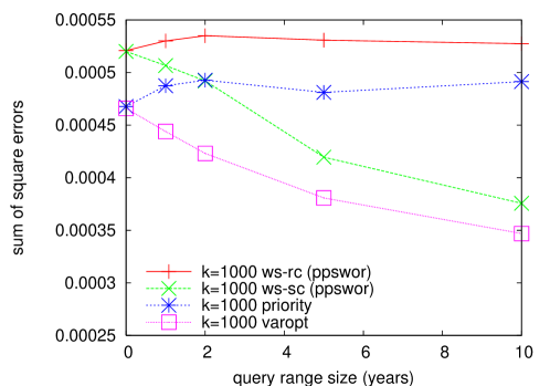
Figure 1: Sum of the square errors of the estimates over each partition, averaged over 500 repetitions of the respective summarization method.

7 Chernoff bounds

In this section we will show that the $\textnormal{\sc VarOpt}_{k}$ schemes from Section 3 provide estimates whose deviations can be bounded with the Chernoff bounds usually associated with independent Poisson samples.

Recall that we defined a $\textnormal{\sc VarOpt}_{k}$ as a sampling scheme with unbiased estimation such that given items $i\in[n]$ with weights $w_{i}$:

(i)

Ipps. We have the sampling probabilities $p_{i}=\min\{1,w_{i}/\tau_{k}\}$ where the threshold $\tau_{k}$ is the unique value such that $\sum_{i\in[n]}\min\{1,w_{i}/\tau_{k}\}=k$ assuming $k<n$; otherwise $\tau_{k}=0$ meaning that all items are sampled. A sampled item $i$ gets the Horvitz-Thompson estimator $\widehat{w}_{i}=w_{i}/p_{i}=\max\{w_{i},\tau_{k}\}$.

(ii)

At most $k$ samples—this hard capacity constraint prevents independent Poisson samples.

(iii)

No positive covariances.

In Section 3 we noted that when $n=k+1$, there is only a unique VarOpt_k scheme; namely VarOpt_k,k+1 which drops one item which is item $i$ with probability $q_{i}=1-p_{i}$ with $p_{i}$ the ipps from (i). We also proved that the VarOpt_k conditions (i)–(iii) are preserved by recurrence (4) stating that

$$\textnormal{\sc VarOpt${}_{k}$}(\bigcup_{x\in[m]}I_{x})=\textnormal{\sc VarOpt${}_{k}$}(\bigcup_{x\in[m]}\textnormal{\sc VarOpt}_{k_{x}}(I_{x}))\ ,$$

where $I_{1},...,I_{m}$ are disjoint non-empty sets of weighted items and $k_{x}\geq k$ for each $x\in[m]$.

In this section, we will show that any scheme generated as above satisfies property (iii$+$) below which can be seen as a higher-order version (iii).

(iii$+$)

High-order inclusion and exclusion probabilities are bounded by the respective product of first-order probabilities. More precisely for any $J\subseteq[n]$,

$$\mbox{(I):}\quad\quad p[J] \leq \prod_{i\in J}p_{i}$$

$$\mbox{(E):}\quad\quad q[J] \leq \prod_{i\in J}q_{i}$$

where $p_{i}$ is the probability that item $i$ is included in the sample $S$ and $p[J]$ is the probability that all $i\in J$ are included in the sample. Symmetrically $q_{i}$ is the probability that item $i$ is excluded from the sample $S$ and $q[J]$ is the probability that all $i\in J$ are excluded from the sample. We will use $X_{i}$ as the indicator variable for $i$ being in the sample, so $\Pr[X_{i}=1]=p_{i}$ and $\Pr[X_{i}=0]=q_{i}$.

It is standard that a special case of Property (iii$+$)(I) implies (iii): For any $i,j$, $p_{i,j}\leq p_{i}p_{j}$ combined with Horvitz-Thompson estimators implies nonnegative covariance between $\widehat{w}_{i}$ and $\widehat{w}_{j}$.

The significance of (iii$+$) was argued by Panconesi and Srinivasan [24] who used it to prove Chernoff bounds that we usually associate with independent Poisson sampling. They did not consider input weights, but took the inclusion probabilities $p_{i}$ as input. For us this corresponds to the special case where the weights sum to $k$ for then we get $p_{i}=w_{i}$. Given the inclusion probabilities $p_{i}$, Srinivasan [28] presented an off-line sampling scheme realizing (i)-(iii+). Strengthening the results from [24, 28] slightly, we prove

Theorem 18

Let $I\subseteq[n]$ and $m=|I|$. For $i\in I$, let $X_{i}$ be a random 0/1 variable which is $1$ with probability $p_{i}$ and $0$ otherwise. The variables may not be independent. Let $X_{I}=\sum_{i\in I}X_{i}$, and $\mu=E[X]=\sum_{i\in I}p_{i}$. Finally let $0<a<m$.

• If (iii$+$)(I) is satisfied and $a\geq\mu$, then

  $$\Pr[X_{I}\geq a]\leq\left(\frac{m-\mu}{m-a}\right)^{m-a}\left(\frac{\mu}{a}\right)^{a}\quad\left[\leq e^{a-\mu}\left(\frac{\mu}{a}\right)^{a}\right]\ .$$ (11)

• If (iii$+$)(E) is satisfied and $a\leq\mu$, then

  $$\Pr[X_{I}\leq a]\leq\left(\frac{m-\mu}{m-a}\right)^{m-a}\left(\frac{\mu}{a}\right)^{a}\quad\left[\leq e^{a-\mu}\left(\frac{\mu}{a}\right)^{a}\right]\ .$$ (12)

7.1 Relevance to VarOpt_k estimates

The above Chernoff bounds only address the number of sampled items while we are interested in estimates of the weight of some subset $H\subseteq[n]$. We split $H$ in a set of heavy items $L=\{i\in H|w_{i}\geq\tau_{k}\}$ and a set of light items $I=H\setminus L=\{i\in H|w_{i}<\tau_{k}\}$. Then our estimate can be written as

$$\widehat{w}_{H}=\sum_{i\in L}w_{i}+\tau_{k}|S\cap I|=\sum_{i\in L}w_{i}+\tau_{k}\sum_{i\in I}X_{i}=w_{L}+\tau_{k}X_{I}\ .$$

Here $X_{I}$ is the only variable part of the estimate and Theorem 18 bounds the probability of deviations in $X_{I}$ from its mean $\mu$. Using these bounds we can easily derive confidence bounds like those in [31] for threshold sampling.

7.2 Satisfying (iii$+$)

In this subsection, we will show that (iii$+$) is satisfied by all the VarOpt_k schemes generated with our recurrence (4). As special cases this includes our VarOpt_k scheme for streams and the schemes of Chao [3] and Tillé [33] schemes. We note that [3, 33] stated only (iii) but (iii$+$)(I) directly follows from the expressions they provide for inclusion probabilities. Condition (iii+) for second order exclusion follows from second order inclusion. In [3, 33] there is no mentioning and no derivation towards establishing (iii$+$)(E) which is much harder to establish than (iii$+$)(I).

Lemma 19

$\textnormal{\sc VarOpt}_{k,k+1}$ satisfies (iii$+$).

Proof

Here $\textnormal{\sc VarOpt}_{k,k+1}$ is the unique VarOpt_k scheme when $n=k+1$. It removes one item $i\in[k+1]$ according to $q_{i}=1-p_{i}$ where $p_{i}$ are the ipps probabilities from (i). Here $\sum_{i}p_{i}=k$ so $\sum_{i}q_{i}=1$. Consider $J\subseteq[k+1]$. If $|J|=1$, (iii$+$) trivially holds. If $|J|>1$, $q[J]=0$ and hence $q[J]\leq\prod_{i\in J}q_{i}$, establishing (iii$+$)(E). Also $p[J]=1-\sum_{i\in J}q_{j}\leq\prod_{j\in J}(1-q_{j})=\prod_{j\in J}p_{j}$, establishing (iii$+$)(I).  

The rest of this subsection is devoted to prove that (iii$+$) is preserved by (4).

Theorem 20

VarOpt defined by (i)-(iii$+$) satisfies recurrence (4):

$$\textnormal{\sc VarOpt${}_{k}$}(\bigcup_{x\in[m]}I_{x})=\textnormal{\sc VarOpt${}_{k}$}(\bigcup_{x\in[m]}\textnormal{\sc VarOpt}_{k_{x}}(I_{x}))\ .$$

where $I_{1},...,I_{m}$ are disjoint and $k_{1},...,k_{m}\geq k$.

We want to show that if each of the subcalls on the right hand side satisfy (i)-(iii$+$), then so does the resulting call. In Section 2.1 we proved this for (i)-(iii) is preserved. It remains to prove that the resulting call satisfies (iii$+$).

We think of the above sampling as divided in two stages. We start with $I=\bigcup_{x\in[m]}I_{x}$. Stage (0) is the combined inner sampling, taking us from $I$ to $I^{(1)}=\bigcup_{x\in[m]}\textnormal{\sc VarOpt}_{k_{x}}(I_{x})$. Stage (1) is the outer subcall taking us from $I^{(1)}$ to the final sample $S=\textnormal{\sc VarOpt${}_{k}$}(I^{(1)})$.

We introduce some notation. For every $i\in I$, we denote by $p^{(0)}[i]$ the probability that $i$ is included in $I^{(1)}$. Then $q^{(0)}[i]=1-p^{(0)}[i]$ is the corresponding exclusion probability. Observe that $p^{(0)}[i]$ and $q^{(0)}[i]$ are the respective inclusion and exclusion probabilities of $i$ in $\textnormal{\sc VarOpt}_{k_{x}}(I_{x})$ for the unique $x$ such that $i\in I_{x}$. For $J\subseteq I$, we use the notation $p^{(0)}[J]=\Pr[J\subseteq I^{(1)}]$ and $q^{(0)}[J]=\Pr[J\cap I^{(1)}=\emptyset]$ for the inclusion and exclusion probabilities of $J$ in $I^{(1)}$. Denote by $p^{(1)}[J|I^{(1)}]$ and $q^{(1)}[J|I^{(1)}]$ the inclusion and exclusion probabilities of $J$ by $\textnormal{\sc VarOpt${}_{k}$}(I^{(1)})$. We denote by $p[J]$ the probability that all items in $J$ are selected for the final sample $S$, and by $q[J]$ the probability that no item of $J$ is selected for $S$.

Our goal is to show that (iii$+$) is satisfied for the final sample $S$. As a first easy step exercising our nation, we show that (iii$+$) satisfied for the sample $I^{(1)}$ resulting from stage (0).

Lemma 21

If the samples of each independent subcall $\textnormal{\sc VarOpt}_{k_{x}}(I_{x})$ satisfies (iii$+$)(I) (respectively, (iii$+$)(E)), then so does their union $I^{(1)}=\bigcup_{x\in[m]}\textnormal{\sc VarOpt}_{k_{x}}(I_{x})$ as a sample of $I$.

Proof

We consider the case of inclusion. Consider $J\subseteq I$. Since $\textnormal{\sc VarOpt}_{k_{x}}(I_{x})$ are independent, we get $p^{(0)}[J]=\prod_{x}p^{(0)}[J_{x}]$ where $J_{x}=J\cap I_{x}$. We assumed (iii$+$)(I) for each $\textnormal{\sc VarOpt}_{k_{x}}(I_{x})$ so $p^{(0)}[J_{x}]\leq\prod_{i\in J_{x}}p^{(0)}[i]$. Substituting we obtain $p^{(0)}[J]=\prod_{i\in J}p^{(0)}[i]$. The proof for exclusion probabilities is symmetric.  
The most crucial property we will need from (i) and (ii) is a certain kind of consistency. Assume some item $i\in I$ survives stage (0) and ends in $I^{(1)}$. We say that overall sampling is consistent if the probability $p^{(1)}[i|I^{(1)}]$ that $i$ survives stage (1) is independent of which other items are present in $I^{(1)}$. In other words, given any two possible values $I^{(1)}_{1}$ and $I^{(1)}_{2}$ of $I^{(1)}$, we have $p^{(1)}[i|I^{(1)}_{1}]=p^{(1)}[i|I^{(1)}_{2}]$, and we let $p^{(1)}[i]$ denote this unique value. Under consistency, we also define $q^{(1)}[i]=1-q^{(1)}[i]$, and get some very simple formulas for the overall inclusion and exclusion probabilities; namely that $p[i]=p^{(1)}[i]\,p^{(0)}[i]$ and $q[i]=q^{(0)}[i]+p^{(0)}[i]\,q^{(1)}[i]$.

Note that even with consistency, when $|J|>1$, $q^{(1)}[J|I^{(1)}]$ and $p^{(1)}[J|I^{(1)}]$ may depend on $I^{(1)}$.

Lemma 22

Consider (4) where the inner subcalls satisfy properties (i) and (ii) and the outer subcall satisfies property (i). Then we have consistent probabilities $p^{(1)}[i]$ and $q^{(1)}[i]$ as defined above.

Proof

Our assumptions are the same as those for Lemma 3, so we know that the threshold $\tau^{\prime}$ of the outer subcall is a unique function of the weights in $I$. Consider any $i\in I$, and let $x$ be unique index such that $i\in I_{x}$. We assume that $i\in\textnormal{\sc VarOpt}_{k_{x}}(I_{x})$, and by (i), we get an adjusted weight of $w^{(1)}_{i}=\max\{w_{i},\tau_{k_{x}}\}$. This value is a function of the weights in $I_{x}$, hence independent of which other items are included in $I^{(1)}$. Be by (i) on the outer subcall, we have that the probability that $i\in I^{(1)}$ survives the final sampling is $\min\{1,w^{(1)}_{i}/\tau^{\prime}\}=\min\{1,\max\{w_{i},\tau_{k_{x}}\}/\tau^{\prime}\}$, hence a direct function of the original weights in $I$.  
By Lemma 21 and 22, the following implies Theorem 20.

Proposition 23

Consider consistent two stage sampling. If both stages satisfy (iii$+$)(I) (resp., (iii$+$)(E)), then so does the composition.

As we shall see below, the inclusion part of Proposition 23 is much easier than the exclusion part.

For $J^{\prime}\subseteq J\subseteq I$, we denote by $\overline{p}^{(0)}[J^{\prime},J]$ the probability that items $J^{\prime}$ are included and items $J\setminus J^{\prime}$ are excluded by stage (0) sampling. In particular, $\overline{p}^{(0)}[I^{(1)},I]$ is the probability that the outcome of stage (0) is $I^{(1)}$. Note that we always have $\overline{p}^{(0)}[J^{\prime},J]\leq p^{(0)}[J^{\prime}]$. We now establish the easy inclusion part (I) of Proposition 23.

Proof of Proposition 23(I)

$$p[J] = \sum_{I^{(1)}\mid J\subseteq I^{(1)}}\overline{p}^{(0)}[I^{(1)},I]p^{(1)}[J|I^{(1)}]$$

$$\leq \sum_{I^{(1)}\mid J\subseteq I^{(1)}}\overline{p}^{(0)}[I^{(1)},I]\prod_{j\in J}p^{(1)}[j]$$

$$= \prod_{j\in J}p^{(1)}[j]p^{(0)}[J]$$

$$\leq \prod_{j\in J}p^{(0)}[j]\prod_{j\in J}p^{(1)}[j]$$

$$= \prod_{j\in J}p^{(0)}[j]p^{(1)}[j]=\prod_{j\in J}p[j]$$

 

Next we establish the much more tricky exclusion part of Proposition 23. First we need

Lemma 24

$$\overline{p}^{(0)}[J^{\prime},J]=\sum_{H\subseteq J^{\prime}}(-1)^{|H|}q^{(0)}[H\cup(J\setminus J^{\prime})]$$ (13)

Proof

Let $B$ be the event that $J\setminus J^{\prime}$ are excluded from the sample. For $j\in J^{\prime}$, let $A_{j}$ be the event that $\{j\}\cup J\setminus J^{\prime}$ are excluded from the sample..

From definitions,

$$\overline{p}^{(0)}[J^{\prime},J]=\Pr[B]-\Pr[\bigcup_{j\in J^{\prime}}A_{j}]\ .$$ (14)

Applying the general inclusion exclusion principle, we obtain

$$\Pr[\bigcup_{j\in J^{\prime}}A_{j}] = \sum_{H\,|\,\emptyset\neq H\subseteq J^{\prime}}(-1)^{|H|+1}\Pr[\bigcap_{j\in H}A_{j}]$$ (15)

$$= \sum_{H\,|\,\emptyset\neq H\subseteq J^{\prime}}(-1)^{|H|+1}q^{(0)}[H\cup(J\setminus J^{\prime})]$$

Now (13) follows using $\Pr[B]=q^{(0)}[J\setminus J^{\prime}]$ and (15) in (14).  
We are now ready to establish the exclusion part (E) of Proposition 23 stating that with consistent two stage sampling, if both stages satisfy (iii$+$)(E), then so does the composition.

Proof of Proposition 23(E)

We need to show that $q[J]\leq\prod_{j\in J}q[j]$

$$q[J] = \sum_{I^{(1)},J^{\prime}=J\cap I^{(1)}}\overline{p}^{(0)}[I^{(1)},I]\,q^{(1)}[J^{\prime}\,|\,I^{(1)}]$$ (16)

$$= \sum_{J^{\prime}\subseteq J}\left(\sum_{I^{(1)}\,|\,I^{(1)}\cap J=J^{\prime}}\overline{p}^{(0)}[I^{(1)},I]q^{(1)}[J^{\prime}|I^{(1)}]\right)$$

$$\leq \sum_{J^{\prime}\subseteq J}\left(\sum_{I^{(1)}\,|\,I^{(1)}\cap J=J^{\prime}}\overline{p}^{(0)}[I^{(1)},I]\prod_{j\in J^{\prime}}q^{(1)}[j|I^{(1)}]\right)$$

$$= \sum_{J^{\prime}\subseteq J}\left(\sum_{I^{(1)}\,|\,I^{(1)}\cap J=J^{\prime}}\overline{p}^{(0)}[I^{(1)},I]\prod_{j\in J^{\prime}}q^{(1)}[j]\right)$$

$$= \sum_{J^{\prime}\subseteq J}\left(\sum_{I^{(1)}\,|\,I^{(1)}\cap J=J^{\prime}}\overline{p}^{(0)}[I^{(1)},I]\right)\prod_{j\in J^{\prime}}q^{(1)}[j]$$

$$= \sum_{J^{\prime}\subseteq J}\overline{p}^{(0)}[J^{\prime},J]\prod_{j\in J^{\prime}}q^{(1)}[j]$$ (18)

Above, for (16), we applied (iii$+$)(E) on stage (1), and for (7.2), we applied consistency. We now apply Lemma 24 to $\overline{p}^{(0)}[J^{\prime},J]$ in (18), and get

$$q[J] \leq \sum_{J^{\prime}\subseteq J}\left(\sum_{H\subseteq J^{\prime}}(-1)^{|H|}\,q^{(0)}[H\cup(J\setminus J^{\prime})]\right)\prod_{j\in J^{\prime}}q^{(1)}[j]$$

$$= \sum_{(L,H,J^{\prime})|H\subseteq L\subseteq J,\;J^{\prime}=H\cup(J\setminus L)}(-1)^{|H|}\,q^{(0)}[L]\prod_{j\in J^{\prime}}q^{(1)}[j]$$

$$= \sum_{L\subseteq J}q^{(0)}[L]\prod_{j\in J\setminus L}q^{(1)}[j]\left(\sum_{H\subseteq L}\prod_{h\in H}\left(-q^{(1)}[j]\right)\right)$$

Note the convention that the empty product $\prod_{h\in\emptyset}\left(-q^{(1)}[h]\right)\equiv 1$. Observe that $\sum_{H\subseteq L}\prod_{h\in H}\left(-q^{(1)}[h]\right)\ =\ \prod_{\ell\in L}\left(1-q^{(1)}[\ell]\right)$ is non-negative. Moreover, from (iii$+$)(E) on stage (0), we have $q^{(0)}[L]\leq\prod_{\ell\in L}q^{(0)}[\ell]$. Hence, we get

$$q[J] \leq \sum_{L\subseteq J}\prod_{\ell\in L}q^{(0)}[\ell]\prod_{j\in J\setminus L}q^{(1)}[j]\left(\sum_{H\subseteq L}\prod_{h\in H}\left(-q^{(1)}[j]\right)\right)$$ (19)

$$= \sum_{(L,H)|H\subseteq L\subseteq J}\ \prod_{\ell\in L\setminus H}q^{(0)}[\ell]\prod_{j\in J\setminus L}q^{(1)}[j]\prod_{h\in H}\left(-q^{(0)}[h]q^{(1)}[h]\right).$$

To prove $q[J]\leq\prod_{j\in J}q[j]$, we re-express $\prod_{j\in J}q[j]$ to show that it is equal to (19).

$$\prod_{j\in J}q[j] = \prod_{j\in J}\left(q^{(0)}[j]+(1-q^{(0)}[j])q^{(1)}[j]\right)$$ (20)

$$= \prod_{j\in J}(q^{(0)}[j]+q^{(1)}[j]-q^{(0)}[j]q^{(1)}[j])$$

Now (20) equals (19) because $(L\setminus H,J\setminus L,H)$ ranges over all 3-partitions of $J$.  
We have now proved both parts of Proposition 23 which together with Lemma 21 and 22 implies Theorem 20. Thus we conclude that any VarOpt_k scheme generated from VarOpt_k,k+1 and recurrence (4) satisfies (i)–(iii$+$).

7.3 From (iii$+$) to Chernoff bounds

We now want to prove the Chernoff bounds of Theorem 18. We give a self-contained proof but many of the calculations are borrowed from [24, 28]. The basic setting is as follows. Let $I\subseteq[n]$ and $m=|I|$. For $i\in I$, let $X_{i}$ be a random 0/1 variable which is $1$ with probability $p_{i}$ and $0$ otherwise. The variables may not be independent. Let $X_{I}=\sum_{i\in I}X_{i}$, and $\mu=E[X]=\sum_{i\in I}p_{i}$. Finally let $0<a<m$. Now Theorem 18 falls in two statements:

• If (iii$+$)(I) is satisfied and $a\geq\mu$, then

  $$\Pr[X_{I}\geq a]\leq\left(\frac{m-\mu}{m-a}\right)^{m-a}\left(\frac{\mu}{a}\right)^{a}$$

• If (iii$+$)(E) is satisfied and $a\leq\mu$, then

  $$\Pr[X_{I}\leq a]\leq\left(\frac{m-\mu}{m-a}\right)^{m-a}\left(\frac{\mu}{a}\right)^{a}$$

We will now show that it suffices to prove Theorem 18 (I).

Lemma 25

Theorem 18 (I) implies Theorem 18 (E).

Proof

Define random 0/1 variables $Y_{i}=1-X_{i}$, $i\in[n]$, let $Y=\sum_{i\in[n]}Y_{i}$, $\gamma=\textsf{E}[Y]$, and $b=m-a$. Note that $Y=m-X$ and $\gamma=m-\mu$. We have that

$$\Pr[X\leq a]=\Pr[m-X\geq m-a]=\Pr[Y\geq b]\ .$$

Now if $X_{i}$ satisfies (iii$+$)(E) then $Y_{i}$ satisfies (iii$+$)(I) so we can apply Theorem 18 (I) to $Y$ and $b$ and get

$$\Pr[Y\geq b]\leq\left(\frac{\gamma}{b}\right)^{b}\left(\frac{m-\gamma}{m-b}\right)^{m-b}\\ =\left(\frac{m-\mu}{m-a}\right)^{n-a}\left(\frac{\mu}{a}\right)^{a}\ ,$$

Hence Theorem 18 (E) follows.  
We will now prove the Chernoff bound of Theorem 18 (E). The traditional proofs of such bounds for $X=\sum X_{i}$ assume that the $X_{i}$s are independent and uses the equality $\textsf{E}[e^{tX}]=\prod_{i}\textsf{E}[e^{tX_{i}}]$. Our $X_{i}$ are not independent, but we have something as good, essentially proved in [24].

Lemma 26

Let $X_{1},...,X_{m}$ be random 0/1 variables satisfying (iii$+$)(I), that is, for any $J\subseteq[n]$,

$$\Pr[\prod_{j\in J}X_{j}=1]\leq\prod_{j\in J}\Pr[X_{j}=1].$$

Let $I\subseteq[n]$ and $X=\sum_{i\in I}X_{i}$. Then for any $t\geq 0$,

$$\textsf{E}[e^{tX}]\leq\prod_{i\in I}\textsf{E}[e^{tX_{i}}].$$

Proof

For simplicity of notation, we assume $I=[m]=\{1,...,m\}$. Let $\widehat{X_{1}},....,\widehat{X_{m}}$ be independent random 0/1 variables with the same marginal distributions as the $X_{i}$, that is, $\Pr[X_{i}=1]=\Pr[\widehat{X_{i}}=1]$. Let $\widehat{X}=\sum_{i\in[m]}\widehat{X_{i}}$. We will prove the lemma by proving

$$\textsf{E}[e^{tX}] \leq \textsf{E}[e^{t\widehat{X}}]$$

$$= \prod_{i\in[m]}\textsf{E}[e^{t\widehat{X_{i}}}]\ =\ \prod_{i\in[m]}\textsf{E}[e^{tX_{i}}]$$

Using Maclaurin expansion $e^{x}=\sum_{k\geq 0}\frac{x^{k}}{k!}$, so for any random variable $X$, $\textsf{E}[e^{tX}]=\sum_{k\geq 0}\frac{t^{k}{\sf E}[X^{k}]}{k!}$. Since $t\geq 0$, (7.3) follows if we for every $k$ can prove that $\textsf{E}[X^{k}]\leq\textsf{E}[\widehat{X}^{k}]$. We have

$$\textsf{E}[X^{k}] = \sum_{j_{1},\ldots,j_{m}\mid j_{1}+\cdots+j_{m}=m}{m\choose{j_{1},\dots,j_{m}}}\textsf{E}[\prod_{i\in[m]}X_{i}^{j_{i}}]$$ (22)

$$= \sum_{j_{1},\ldots,j_{m}\mid j_{1}+\cdots+j_{m}=m}{m\choose{j_{1},\dots,j_{m}}}\textsf{E}[\prod_{i\in[m]|j_{i}\geq 1}X_{i}]$$ (23)

$$\leq \sum_{j_{1},\ldots,j_{m}\mid j_{1}+\cdots+j_{m}=m}{m\choose{j_{1},\dots,j_{m}}}\prod_{i\in[m]|j_{i}\geq 1}\textsf{E}[X_{i}]$$ (24)

$$= \sum_{j_{1},\ldots,j_{m}\mid j_{1}+\cdots+j_{m}=m}{m\choose{j_{1},\dots,j_{m}}}\prod_{i\in[m]}\textsf{E}[X_{i}^{j_{i}}]$$

$$= \sum_{j_{1},\ldots,j_{m}\mid j_{1}+\cdots+j_{m}=m}{m\choose{j_{1},\dots,j_{m}}}\prod_{i\in[m]}\textsf{E}[\widehat{X}_{i}^{j_{i}}]$$

$$= \textsf{E}[\widehat{X}^{k}]\ ,$$ (26)

Here (22) and (26) follow from linearity of expectation, (23) and (7.3) follow from the fact that if $X_{i}$ is a random 0/1 variable then for $j\geq 1$, $X_{i}^{j}=X_{i}$, and (24) follows using (iii$+$)(I). Hence $\textsf{E}[e^{tX}]\leq\textsf{E}[e^{t\widehat{X}}]$ as claimed in (7.3).  
Using Lemma 26, we can mimic the standard proof of Theorem 18 (I) done with independent variables.

Proof of Theorem 18 (I)

For every $t>0$

$$\Pr[X\geq a]=\Pr[e^{tX}\geq e^{ta}]\ .$$

Using Markov inequality it follows that

$$\Pr[X\geq a]\leq\frac{\textsf{E}[e^{tX}]}{e^{ta}}\ .$$ (27)

Using Lemma 26 and arithmetic-geometric mean inequality, we get that

$$\textsf{E}[e^{tX}] \leq \prod_{i\in[n]}\textsf{E}[e^{tX_{i}}]$$

$$= \prod_{i\in[n]}\left(1+p_{i}(e^{t}-1)\right)$$

$$\leq \left(\frac{\sum_{i\in[n]}(1+p_{i}(e^{t}-1))}{m}\right)^{m}$$

$$= \left(1+\frac{\mu}{m}(e^{t}-1)\right)^{m}$$

Substituting this bound into Equation (27) we get that

$$\Pr[X\geq a]\leq\frac{\left(1+\frac{\mu}{m}(e^{t}-1)\right)^{m}}{{e^{t\,a}}}\ .$$ (28)

Substituting

$$e^{t}=\frac{a(n-\mu)}{\mu(n-a)}$$

into the right hand side of Equation (28) we obtain that

$$\Pr[X\geq a]\leq\frac{\left(1+\frac{\mu}{m}\left(\frac{a(n-\mu)}{\mu(n-a)}-1\right)\right)^{m}}{{\left(\frac{a(n-\mu)}{\mu(n-a)}\right)^{a}}}=\frac{\left(\frac{m-\mu}{m-a}\right)^{m}}{{\left(\frac{a(n-\mu)}{\mu(m-a)}\right)^{a}}}=\left(\frac{n-\mu}{m-a}\right)^{m-a}\left(\frac{\mu}{a}\right)^{a}\ ,$$

as desired.  
In combination with Lemma 25 this completes the proof of Theorem 18. As described in Section 7.1, this implies that we can use the Chernoff bounds (11) and (12) to bound the probability of deviations in our weight estimates.

7.4 Concluding remarks

We presented a general recurrence generating VarOpt_k schemes for variance optimal sampling of $k$ items from a set of weighted items. The schemes provides the best possible average variance over subsets of any given size. The recurrence covered previous schemes of Chao and Tillé [3, 33], but it also allowed us to derive very efficient VarOpt_k schemes for a streaming context where the goal is to maintain a reservoir with a sample of the items seen thus far. We demonstrated the estimate quality experimentally against natural competitors such as ppswor and priority sampling. Finally we showed that the schemes of the recurrence also admits the kind Chernoff bounds that we normally associate with independent Poisson sampling for the probability of large deviations.

In this paper, each item is indepdenent. In subsequent work [5], we have considered the unaggregated case where the stream of item have keys, and where we are interested in the total weight for each key. Thus, instead of sampling items, we sample keys. As we sample keys for the reservoir, we do not know which keys are going to reappear in the future, and for that reason, we cannot do a variance optimal sampling of the keys. Yet we use the variance optimal sampling presented here as a local subroutine. The result is a heuristic that in experiments outperformed classic schemes for sampling of unaggregated data like sample-and-hold [14, 17].

Appendix A Auxiliary variables

Continuing from Section 1.4 we now consider the case where we for each item are interested in an auxiliary weight $w^{\prime}_{i}$. For these we use the estimate

$${\widehat{w}}^{\prime}_{i}=w^{\prime}_{i}\widehat{w}_{i}/w_{i}$$

Let ${V\Sigma}^{\prime}=\sum_{i\in[n]}{\widehat{w}}^{\prime}_{i}$ be the variance on the estimate of the total for the auxiliary variables. We want to argue that we expect to do best possible on ${V\Sigma}^{\prime}$ using VarOpt_k that minimizes ${\Sigma}V$ and ${V\Sigma}$, assuming that the $w^{\prime}_{i}$ are randomly generated from the $w_{i}$. Formally we assume each $w^{\prime}_{i}$ is generated as

$$w^{\prime}_{i}=x_{i}w_{i}$$

where the $x_{i}$ is drawn independently from the same distribution $\Xi$. We consider expectations $\textsf{E}_{\Xi}$ for given random choices of the $x_{i}$, that is, formally

$$\textsf{E}_{\Xi}[{V\Sigma}^{\prime}]=\textsf{E}_{x\leftarrow\Xi,i\in[n]}\left[{V\Sigma}^{\prime}\,|\,x\right]$$

We want to prove (2)

$$\textsf{E}_{\Xi}[{V\Sigma}^{\prime}]=\mathop{\sf Var}[\Xi]{\Sigma}V+\textsf{E}[\Xi]^{2}{V\Sigma}\textnormal{,}$$

where $\mathop{\sf Var}[\Xi]=\mathop{\sf Var}_{\Xi}[x_{i}]$ and $\textsf{E}[\Xi]=\textsf{E}_{\Xi}[x_{i}]$ for every $x_{i}$. Note that if the $x_{i}$ are 0/1 variables, then the ${\widehat{w}}^{\prime}_{i}$ represent a random subset, including each item independently. This was one of the cases considered in [30]. However, the general scenario is more like that in statistics where we can think of $w_{i}$ as a known approximation of a real weight $w^{\prime}_{i}$ which only becomes known if $i$ is actually sampled. As an example, consider house hold incomes. The $w_{i}$ could be an approximation based on street address, but we only find the real incomes $w^{\prime}_{i}$ for those we sample. What (2) states is that if the $w_{i}^{\prime}$ are randomly generated from the $w_{i}$ by multiplication with independent identically distributed random numbers, then we minimize the expected variance on the estimate of the real total if our basic scheme minimizes ${\Sigma}V$ and ${V\Sigma}$.

To prove (2), write

$${V\Sigma}^{\prime}={\Sigma}V^{\prime}+{\Sigma}CoV^{\prime}\quad\mbox{where}\quad{\Sigma}V^{\prime}=\sum_{i\in[n]}\mathop{\sf Var}[\widehat{w}^{\prime}_{i}]\quad\mbox{and}\quad{\Sigma}CoV^{\prime}=\sum_{i,j\in[n]\,|\,i\neq j}\mathop{\mathsf{Cov}}[\widehat{w}^{\prime}_{i},\widehat{w}^{\prime}_{j}].$$

Here $\mathop{\sf Var}[\widehat{w}^{\prime}_{i}]=x_{i}^{2}\mathop{\sf Var}[\widehat{w}_{i}]$ so $\textsf{E}_{\Xi}[\mathop{\sf Var}[\widehat{w}^{\prime}_{i}]]=\textsf{E}_{\Xi}[x_{i}^{2}]\mathop{\sf Var}[\widehat{w}_{i}]$, so by linearity of expectation,

$$\textsf{E}_{\Xi}[{\Sigma}V^{\prime}]=\textsf{E}[\Xi^{2}]{\Sigma}V.$$

Similarly, $\mathop{\mathsf{Cov}}[\widehat{w}^{\prime}_{i},\widehat{w}^{\prime}_{j}]=x_{i}x_{j}\mathop{\mathsf{Cov}}[\widehat{w}_{i},\widehat{w}_{j}]$ so $\textsf{E}_{\Xi}[\mathop{\mathsf{Cov}}[\widehat{w}^{\prime}_{i},\widehat{w}^{\prime}_{j}]]=\textsf{E}_{\Xi}[x_{i}]\textsf{E}_{\Xi}[x_{j}]\mathop{\mathsf{Cov}}[\widehat{w}_{i},\widehat{w}_{j}]$, so by linearity of expectation,

$$\textsf{E}_{\Xi}[{\Sigma}CoV^{\prime}]=\textsf{E}[\Xi]^{2}{\Sigma}CoV=\textsf{E}[\Xi]^{2}({V\Sigma}-{\Sigma}V).$$

Thus

$$\textsf{E}_{\Xi}[{V\Sigma}^{\prime}]=\textsf{E}_{\Xi}[{\Sigma}V^{\prime}]+\textsf{E}_{\Xi}[{\Sigma}CoV^{\prime}]=\textsf{E}[\Xi^{2}]{\Sigma}V+\textsf{E}[\Xi]^{2}({V\Sigma}-{\Sigma}V)=\mathop{\sf Var}[\Xi^{2}]{\Sigma}V+\textsf{E}[\Xi]^{2}{V\Sigma}\textnormal{,}$$

as desired.

Appendix B Bad case for ppswor

We will now provide a generic bad instance for probability proportional to size sampling without replacement (ppswor) sampling $k$ out of $n$ items. Even if ppswor is allowed $k+(\ln k)/2$ samples, it will perform a factor $\Omega(\log k)$ worse on the average variance for any subset size $m$ than the optimal scheme with $k$ samples. Since the optimal scheme has ${V\Sigma}=0$, it suffices to prove the statement concerning ${\Sigma}V$. The negative result is independent of the ppswor estimator as long as unsampled items get estimate $0$. The proof of this negative result is only sketched below.

Let $\ell=n-k+1$. The instance has $k-1$ items of size $\ell$ and $\ell$ unit items. The optimal scheme will pick all the large items and one random unit item. Hence ${\Sigma}V$ is $\ell(1-1/\ell)\ell<\ell^{2}$.

Now, with ppswor, there is some probability that a large item is not picked, and when that happens, it contributes $\ell^{2}$ to the variance. We will prove that with the first $k$ ppswor samples, we waste approximately $\ln k$ samples on unit items, which are hence missing for the large items, and even if we get half that many extra samples, the variance contribution from missing large items is going to be $\Omega(\ell^{2}\log k)$.

For the analysis, suppose we were going to sample all items with ppswor. Let $u_{i}$ be the number of unit items we sample between the $i-1$st and the $i$th large item. Each sample we get has a probability of almost $(k-i)/(k-i+1)$ of being large. We say almost because there may be less than $\ell$ remaining unit items. However, we want to show w.h.p. that close to $\ln k$ unit items are sampled, so for a contradiction, we can assume that at least $\ell-\ln k\approx\ell$ unit items remain. As a result, the expected number of unit items in the interval is $(k-i+1)/(k-i)-1=1/(k-i)$. This means that by the time we get to the $k-\lceil\ln k\rceil$th large item, the expected number of unit samples is $\sum_{i=1}^{k-\lceil\ln k\rceil}1/(k-i)\approx\ln k$. Since we are adding almost independent random variables each of which is at most one, we have a sharp concentration, so by the time we have gotten to the $k-\lceil\ln k\rceil$ large item, we have approximately $\ln k$ unit samples with high probability.

To get a formal proof using Chernoff bounds, for the number of unit items between large item $i-1$ and $i$, we can use a pessimistic 0/1 random variable dominated be the above expected number. This variable is 1 with probability $1/(k-i+1)(1-\ln k/\ell)$ which is less than the probability that the next item is small, and now we have independent variables for different rounds.

References

- [1] R.J Adler, R.E. Feldman, and M.S. Taqqu. A Practical Guide to Heavy Tails. Birkhauser, 1998.
- [2] S. Alstrup, T. Husfeldt, and T. Rauhe. Marked ancestor problems. In Proc. 39th FOCS, pages 534–544, 1998.
- [3] M. T. Chao. A general purpose unequal probability sampling plan. Biometrika, 69(3):653–656, 1982.
- [4] S. Chaudhuri, R. Motwani, and V.R. Narasayya. On random sampling over joins. In Proc. ACM SIGMOD Conference, pages 263–274, 1999.
- [5] E. Cohen, N.G. Duffield, H. Kaplan, C. Lund, and M. Thorup. Composable, scalable, and accurate weight summarization of unaggregated data sets. Proc. VLDB, 2(1):431–442, 2009.
- [6] E. Cohen and H. Kaplan. Bottom-k sketches: Better and more efficient estimation of aggregates (poster). In Proc. ACM SIGMETRICS/Performance, pages 353–354, 2007.
- [7] E. Cohen and H. Kaplan. Summarizing data using bottom-k sketches. In Proc. 26th ACM PODC, 2007.
- [8] E. Cohen and H. Kaplan. Tighter estimation using bottom-k sketches. In Proceedings of the 34th VLDB Conference, 2008.
- [9] Th. H. Cormen, Ch. E. Leiserson, R. L. Rivest, and C. Stein. Introduction to algorithms. MIT Press, McGraw-Hill, 2nd edition, 2001.
- [10] C. Cranor, T. Johnson, V. Shkapenyuk, and O. Spatcheck. Gigascope: A stream database for network applications. In Proc. ACM SIGMOD, 2003.
- [11] N.G. Duffield, C. Lund, and M. Thorup. Learn more, sample less: control of volume and variance in network measurements. IEEE Transactions on Information Theory, 51(5):1756–1775, 2005.
- [12] N.G. Duffield, C. Lund, and M. Thorup. Priority sampling for estimation of arbitrary subset sums. J. ACM, 54(6):Article 32, December, 2007. Announced at SIGMETRICS’04.
- [13] P. S. Efraimidis and P. G. Spirakis. Weighted random sampling with a reservoir. Inf. Process. Lett., 97(5):181–185, 2006.
- [14] C. Estan and G. Varghese. New directions in traffic measurement and accounting. In Proceedings of the ACM SIGCOMM’02 Conference. ACM, 2002.
- [15] C.T. Fan, M.E. Muller, and I. Rezucha. Development of sampling plans by using sequential (item by item) selection techniques and digital computers. J. Amer. Stat. Assoc., 57:387–402, 1962.
- [16] Michael L. Fredman and Michael E. Saks. The cell probe complexity of dynamic data structures. In Proc. 21st STOC, pages 345–354, 1989.
- [17] M. Gibbons and Y. Matias. New sampling-based summary statistics for improving approximate query answers. In SIGMOD. ACM, 1998.
- [18] D. G. Horvitz and D. J. Thompson. A generalization of sampling without replacement from a finite universe. J. Amer. Stat. Assoc., 47(260):663–685, 1952.
- [19] T. Johnson, S. Muthukrishnan, and I. Rozenbaum. Sampling algorithms in a stream operator. In Proc. ACM SIGMOD, pages 1–12, 2005.
- [20] D.E. Knuth. The Art of Computer Programming, Vol. 2: Seminumerical Algorithms. Addison-Wesley, 1969.
- [21] D. Moore, V. Paxson, S. Savage, C. Shannon, S. Staniford, and N. Weaver. Inside the slammer worm. IEEE Security and Privacy Magazine, 1(4):33–39, 2003.
- [22] S. Muthukrishnan. Data streams: Algorithms and applications. Foundations and Trends in Theoretical Computer Science, 1(2), 2005.
-
[23]
The Netflix Prize.
http://www.netflixprize.com/. - [24] A. Panconesi and A. Srinivasan. Randomized distributed edge coloring via an extension of the chernoff-hoeffding bounds. SIAM J. Comput., 26(2):350–368, 1997.
- [25] K. Park, G. Kim, and M. Crovella. On the relationship between file sizes, transport protocols, and self-similar network traffic. In Proc. 4th IEEE Int. Conf. Network Protocols (ICNP), 1996.
- [26] M. Pǎtraşcu, 2009. Personal communication.
- [27] C-E. Särndal, B. Swensson, and J. Wretman. Model Assisted Survey Sampling. Springer, 1992.
- [28] A. Srinivasan. Distributions on level-sets with applications to approximation algorithms. In Proc. 41st FOCS, pages 588–597. IEEE, 2001.
- [29] M. Szegedy. The DLT priority sampling is essentially optimal. In Proc. 38th STOC, pages 150–158, 2006.
- [30] M. Szegedy and M. Thorup. On the variance of subset sum estimation. In Proc. 15th ESA, LNCS 4698, pages 75–86, 2007.
- [31] M. Thorup. Confidence intervals for priority sampling. In Proc. ACM SIGMETRICS/Performance, pages 252–253, 2006.
- [32] M. Thorup. Equivalence between priority queues and sorting. J. ACM, 54(6):Article 28, December, 2007. Announced at FOCS’02.
- [33] Y. Tillé. An elimination procedure for unequal probability sampling without replacement. Biometrika, 83(1):238–241, 1996.
- [34] Y. Tillé. Sampling Algorithms. Springer, New York, 2006.
- [35] J.S. Vitter. Random sampling with a reservoir. ACM Trans. Math. Softw., 11(1):37–57, 1985.