Inferring Neuronal Network Connectivity from Spike Data: A Temporal Data Mining Approach

Abstract

Understanding the functioning of a neural system in terms of its underlying circuitry is an important problem in neuroscience. Recent developments in electrophysiology and imaging allow one to simultaneously record activities of hundreds of neurons. Inferring the underlying neuronal connectivity patterns from such multi-neuronal spike train data streams is a challenging statistical and computational problem. This task involves finding significant temporal patterns from vast amounts of symbolic time series data. In this paper we show that the frequent episode mining methods from the field of temporal data mining can be very useful in this context. In the frequent episode discovery framework, the data is viewed as a sequence of events, each of which is characterized by an event type and its time of occurrence and episodes are certain types of temporal patterns in such data. Here we show that, using the set of discovered frequent episodes from multi-neuronal data, one can infer different types of connectivity patterns in the neural system that generated it. For this purpose, we introduce the notion of mining for frequent episodes under certain temporal constraints; the structure of these temporal constraints is motivated by the application. We present algorithms for discovering serial and parallel episodes under these temporal constraints. Through extensive simulation studies we demonstrate that these methods are useful for unearthing patterns of neuronal network connectivity.

Keywords : Spike data Analysis, Temporal data mining, frequent episodes, temporal constraints, neuronal connectivity patterns, synfire chains

1 Introduction

Over the last couple of decades, biology has thrown up many interesting and challenging computational problems. For example, the problem of understanding genome data and protein function has motivated development of many computational and statistical techniques leading to the creation of the interdisciplinary area of Bioinformatics. One of the main driving forces in this case is the availability of large amounts of data, from gene or protein sequencing experiments, and the consequent need for efficient techniques to analyze the data to arrive at reasonable and useful inferences. To solve these computational problems, some techniques developed in other contexts (e.g., Hidden Markov Models, Dynamic Programming) have proved to be quite suitable, after some modifications.

In this paper, we focus on an equally challenging computational problem in another sub area of biology, namely neuroscience. We look at the problem of analyzing multi-neuronal spike train data and suggest that certain techniques from the field of Temporal Data mining are attractive here.

Neurons form the basic computing elements of brain and hence, gaining an understanding of the coordinated behavior of groups of neurons (at different levels of organization) is essential for gaining a principled understanding of brain function. Thus, one of the important problems in neuroscience is that of understanding the functioning of a neural tissue in terms of interactions among its neurons. Many neurons communicate with each other through characteristic electric pulses called action potentials or spikes. Hence one can study the activity of a specific neural tissue by gathering data in the form of sequences of action potentials or spikes generated by each of a group of potentially interconnected neurons. Such data is known as multi-neuronal spike train data. (See section 2 for more details).

Over the past twenty years or so, increasingly better methods are becoming available for simultaneously recording the activities of many neurons. By using techniques such as micro electrode arrays, imaging of currents, voltages, and ionic concentrations etc., spike data can be recorded simultaneously from hundreds of neurons [50, 21, 39, 6]. Vast amounts of such data is now routinely gathered from different neuronal systems. For example, in [6] the authors describe experiments where tens of cortical cultures are maintained for over five weeks and on each day the spiking activities of neurons (both with and without external stimulation) in each culture are recorded for tens of minutes. Each recording session contains data with tens of thousands of spikes. Such multi-neuronal spike train data can now be obtained in vitro from neuronal cultures or in vivo from brain slices, awake behaving animals, and even humans. Such spike train data is a mixture of the stochastic spiking activities of individual neurons as well as correlated spiking activity due to interactions or connections among neurons.

Availability of such data motivates development of efficient techniques for analyzing the spike train data [11]. The computational challenge is to make reasonable inferences regarding the connectivity information or the microcircuits present in the neuronal tissue. The grand objective is to come out with a host of data processing and analysis techniques that would enable reliable inference of the underlying functional connectivity patterns which characterize the microcircuits in the neuronal systems [11]. Like in the field of Bioinformatics, this endeavor also entails an interdisciplinary approach and we may call such an approach as Neuroinformatics. The main objective of this paper is to show that techniques from Temporal Data mining could offer novel and useful points of view for tackling some of the issues involved in analyzing spike train data.

Temporal data mining is concerned with analyzing symbolic data streams with temporal dependencies to discover ‘interesting’ temporal patterns [44, 13, 25, 26, 24]. Temporal data mining differs from classical time series analysis in the kind of information that one seeks to discover. The exact model parameters (e.g. coefficients of an ARMA model or the weights of a recurrent neural network) are of little interest. Unearthing interesting trends or patterns in the data (which are much more readily interpretable by the data owner), is of primary interest. Here we focus on the frequent episodes framework of temporal data mining [19, 43, 41]. In this framework, we view the input data as a sequence of events with each event characterized by an event type and a time of occurrence. The patterns to be discovered are called episodes. (See Sec. 3 for more details). This framework is found useful in many engineering applications. For example, the sequence of fault records logged in a manufacturing process can be viewed as a data stream of events. Then the episodes capture faults with temporal correlations and hence frequent episode discovery can be useful in root cause diagnosis [41].

The multi-neuronal spike train data can also be viewed as a sequential or time-ordered data stream of events where each event is a spike at a particular time and the event type is the neuron that generated the spike. Since functionally interconnected neurons tend to fire in certain precise patterns, discovering frequent episodes in such temporal data can help understand the underlying neural circuitry. In this paper we present some novel techniques for frequent episode discovery and show their utility for the analysis of multi-neuronal spike train data.

Most of the currently proposed methods for analyzing spike train data rely on quantities that can be computed through cross correlations among spike trains (time shifted with respect to one another) [11]. Most of these methods are not computationally efficient for discovering temporal patterns that involve more than a few neurons. (See Sec 2 for a review of spike data analysis). Here we show that the temporal data mining approach of frequent episode discovery is very effective for coming up with reasonable hypotheses regarding the connectivity pattern. Though data mining has been successful in unearthing interesting patterns in large databases in many engineering applications, to the best of our knowledge, this is the first time a data mining technique is explored for spike train data analysis. In our opinion, there are mainly two reasons why a data mining approach is attractive for this problem. Firstly, these techniques are known to be efficient in tackling the combinatorial explosion while looking for patterns in large data sets. Thus, we would be able to efficiently discover patterns involving many neurons also. Secondly, these techniques are essentially model independent in the sense that the discovery algorithms do not need to make many assumptions about the kind of interactions among the neurons in terms of, e.g., parameterized classes of models. The empirical results we present here illustrate both these aspects.

The rest of the paper is organized as follows. We explain the problem of analyzing multi-neuronal spike train data in Section 2. We then present a brief overview of the frequent episodes framework in Section 3. We also introduce a framework of imposing some temporal constraints on the episode occurrences which will be needed in the multi-neuronal data analysis. We end this section with a discussion that explains how one can use methods of serial and parallel episode discovery, under temporal constraints, to discover many patterns of interest in the spike train data. While there are many efficient algorithms for discovering frequent episodes, none of these can directly handle the kind of temporal constraints that are needed in this application. We present some novel algorithms for discovering frequent episodes under temporal constraints in Section 4. We present some simulation results to illustrate our method of discovering connection patterns in neuronal networks in Section 5. For this we have built a simulator for generating spike train data by modeling each neuron as an inhomogeneous Poisson process whose firing rate changes as a function of input spikes it receives from other neurons. We choose two different functional forms for changing the firing rate as a function of input received by a neuron so as to illustrate that our discovery algorithms and their effectiveness in inferring connectivity patterns, are not dependent on any specific mechanism of interactions among neurons. The simulator generates fairly realistic spike data and it allows us to validate the algorithms presented here. We also discuss some results on data from cortical cultures. Finally, we conclude the paper in Section 6.

2 Multi-neuronal Spike Train Data and Its Analysis

The brain or the nervous system consists essentially of a vast network of neurons. The neuron may be regarded as the basic computing element in the nervous system. Each neuron is connected to many others through what are known as synapses. Synapses, through electric and chemical means, allow neurons to signal to each other in the sense that the output of one neuron can become input to another through the synapse that connects them. In a good majority of all neurons, the output of a neuron is in the form of what is called an action potential. An action potential is an electrical signal of a short duration (typically less than 1 ms) with a characteristic shape. For most purposes of analysis, this can be regarded as a short pulse and hence is also referred to as a spike. After generating an action potential, a neuron can not immediately generate another spike because it needs some regenerative time. This time period is called refractory period and in many cases it is in the range of 1 milli second (ms). Over short durations of time the spiking activity of a neuron can be well modeled by a Poisson process whose rate depends on the current state of the neuron. The spikes output by one neuron reach the input terminals of other neurons through the synapses that interconnect them. Each neuron has many such synapses and based on the amount of input it receives like this, it may then fire an action potential or a spike. The functioning of the nervous system is essentially due to this coordinated activity of many neurons. (See, e.g., [36] for a good exposition). The system is stochastic and neurons would also be spiking randomly. The signal transmission through synapses takes some time and thus there are characteristic delays associated with each synapse. Also different synapses may have different efficacies in effecting spikes from the receiving neurons.

Experimental studies for understanding brain function span a wide range of organizational levels. At one end are studies aimed at understanding the functioning of single neurons through electro physiological recordings while at the other end, using techniques such as fMRI, one studies interactions among large brain regions. Our interest in this paper is in experimental techniques at an intermediate level of organization where one is interested in understanding how groups of a few hundred neurons act in a coordinated manner to generate specific functions. For this, as mentioned earlier, one obtains simultaneous recordings of the spikes generated by a group of interacting neurons. By simultaneous recording we mean that the times of spikes of all neurons are referenced with respect to a common time origin and hence the data is suitable for studying temporal interactions among the neurons.

There has been a lot of work on experiments for simultaneously recording the activities of hundreds of neurons for gaining a better understanding of the functional interactions among neurons in a neural tissue [29, 34, 33, 30, 16, 22, 50, 46, 6]. The recording techniques fall into three broad categories. In the first category are recordings from cultured neurons or brain slices using Micro electrode arrays (MEAs). A typical MEA setup for this consists of $8\times 8$ grid of 64 electrodes with inter-electrode spacing of about 100 microns. This allows stimulation of the neural tissue and recording of the resulting spikes using the same set of electrodes [6, 35]. In the second category are recordings from intact animals using MEAs and other probes [39, 21, 30, 22]. In the third category are imaging techniques using voltage sensitive dyes and indicators for ions such as Ca++ [50, 47]. One of the most exciting recent developments is the incorporation of ion-selective pores into neurons of behaving animals [15, 49]. This allows simultaneous stimulation and recording with milli-second precision using light at various wavelengths. All these technologies now allow for gathering of vast amounts of data, using which one wishes to study connectivity patterns and microcircuits in neural systems.

In this paper our interest is in techniques for analyzing the data that is in the form of spike trains. To obtain such spike trains from the recorded data, one needs a lot of signal processing and data preprocessing techniques. For example, in MEA experiments, the raw data is in the form of voltage or current signals from each of the electrodes, recorded at a suitably high sampling rate. By employing appropriate signal processing techniques one has to first reliably locate all spiking events. Even after this, what we have are spike events in each channel or each electrode. Since the micro electrode array is regular while the neuronal tissue is not, each electrode may be picking up signals from many neurons with different efficacies. If we want the final data as spike events generated by individual neurons then we have to do what is called spike sorting. Many techniques have been suggested for processing the raw signals to obtain spikes and to do spike sorting and there is need for better algorithms for these problems. (See, e.g., [11] and references therein). Here we will not review any of these techniques because our interest is in analysis methods that look at spike trains to infer connectivity patterns.

The field of multi-neuronal data analysis has a long history, beginning with the work of Gerstien and his colleagues [18, 7, 29, 17]. A major goal of such neural data analysis is to characterize how neurons that are part of an ensemble interact with each other. Statistical analysis of spike train data was pioneered by Brillinger [8] and the recent review by Kass, Ventura, and Brown [38] addresses all the statistical issues in this area. The review by Brown, Kass, and Mitra [11] summarizes three decades of methodology development in this area and eloquently lays out future challenges. Many of the current methods essentially use information obtained from cross correlation among spike trains that are shifted in time with respect to one another [11]. For example, one can compute what is called a joint peri-stimulus time histogram (JPSTH) which is a two dimensional histogram that displays the joint spike count of two neurons at different time lags (for a specific binning on the time axis). There are other methods based on analyzing time-shifted spike trains for detecting repeated patterns of firing of a few neurons with constant time lags [29, 28, 20]. Given some specific patterns there are methods to look for matches in the spike train data and assess the statistical significance [3]. For assessing the statistical significance of the detected patterns, one generally employs a null hypothesis that the spike trains are iid Bernoulli processes or uses some resampling methods of generating surrogate data streams to assess significance empirically [16, 29, 3]. Most of these techniques are not efficient for detecting patterns involving more than four or five neurons. Another approach is to employ dimensionality reduction techniques such as PCA and study the data in some appropriate low dimensional feature space [47]. Bayesian model estimation techniques have also been used to infer parameters of an assumed statistical model of interaction among neurons [14].

The availability of vast amounts data means that developing efficient methods to analyze neuronal spike trains is a challenging task of immediate utility in this area [11]. To quote Brown, Kass, and Mitra [11], “Simultaneous recording of multiple spike trains from several neurons offers a window into how neurons work in concert to generate specific brain functions. Without substantial methodology research in the future, our ability to understand this function will be significantly hampered because current methods fall short of what is ultimately required for the analysis of multiple spike train data.”

The objective of analyzing spike train data is to finally be able to infer the microcircuits and relate the functioning of neural systems to specific coordinated activities or characteristic firing patterns [48, 27]. In this paper we address the simpler problem of inferring some useful temporal patterns in the spike trains that help understand the connectivity structure.

The characteristics of patterns that one is interested in can be roughly grouped into Synchrony, Order, Synfire chains, and Synfire braids. Synchronous firing by a group of neurons is interesting because it can be an efficient way to transmit information [46, 5, 31]. Ordered or sequential firing of neurons where the time-delays between firing of successive neurons are fairly constant denote a chain of triggering events and unearthing such relations between neurons can thus reveal underlying functional connectivity [28]. If neuron A is functionally connected to neuron B, it influences the firing of neuron B. If this is an excitatory connection (with or without a delay), then, if A fires, B is likely to fire soon after that. Hence, discovering the order of neuronal firings (along with the delays involved) can help decipher the functional connectivity. Memory traces are probably embedded in such sequential activations of neurons or neuronal groups. Signals of this form have recently been found in groups of hippocampal neurons by Lee and Wilson [4]. An ordered chain of firings of neuronal groups (rather than single neurons) is sometimes called a Synfire chain and is believed to be an important microcircuit [27, 50]. A synfire chain can be thought of as a compound pattern involving both synchrony and order. Synfire braids, also called Polychronous chains, are generalizations of Synfire chains. Here, a group of neurons are activated in fairly precise temporal relationships and automatic discovery of these polychronous circuits are considered a very difficult task [10].

Discovering such temporal patterns in spike trains amounts to unearthing groups of neurons that fire in some kind of coordinated fashion. As already mentioned, in most of the currently available methods, the curse of dimensionality forces the analysis to be confined to a few variables at a time. For the same reason, it is often very difficult to discover all patterns of a particular kind. Thus, many of the available algorithms are for counting occurrences of specific list of patterns. In the next section we explain the idea of frequent episodes and show that this data mining viewpoint gives us a unified algorithmic scheme for discovering many types of interesting patterns in spike train data.

3 Frequent Episode Discovery

Frequent episode discovery framework was proposed by Mannila et.al. [19] in the context analyzing alarm sequences in a communication network. Laxman et.al. [43] introduced the notion of non-overlapped occurrences as episode frequency and proposed efficient counting algorithms. We first give brief overview of this framework.

The data to be analyzed is a sequence of events denoted by $\langle(E_{1},t_{1}),(E_{2},t_{2}),\ldots\rangle$ where $E_{i}$ represents an event type and $t_{i}$ the time of occurrence of the $i^{th}$ event. $E_{i}$’s are drawn from a finite set of event types, $\zeta$. The sequence is ordered with respect to time of occurrences of the events so that, $t_{i}\leq t_{i+1}$, for all $i=1,2,\ldots$. The following is an example event sequence containing 9 events with 5 event types.

$$\langle(A,1),(B,3),(D,4),(C,6),(B,8),(A,10),(E,14),(B,15),(C,18)\rangle$$ (1)

In multi-neuron data, a spike event has the label of the neuron (or the electrode number when we consider multi-electrode array recordings without the spike sorting step) which generated the spike as its event type and has the associated time of occurrence. The neurons in the ensemble under observation fire action potentials at different times, that is, generate spike events. All these spike events are strung together, in time order, to give a single long data sequence as needed for frequent episode discovery.

The general temporal patterns that we wish to discover in this framework are called episodes. In this paper we shall deal with two types of episodes: Serial and Parallel.

Formally, an episode $\alpha$ is a triple $(V_{\alpha},\leq_{\alpha},g_{\alpha})$, where $V_{\alpha}$ is a set of nodes, $\leq_{\alpha}$ is a partial order on $V_{\alpha}$, and $g_{\alpha}:V_{\alpha}\rightarrow\zeta$, is a mapping associating each node with an event type. The size of $\alpha$, denoted as $|\alpha|$, is $|V_{\alpha}|$ (i.e. the number of nodes in $V_{\alpha}$). Episode $\alpha$ is a parallel episode if the partial order $\leq_{\alpha}$ is a null set. It is a serial episode if the relation $\leq_{\alpha}$ is a total order. A non-empty partial order which is neither a total order nor a null set corresponds to a general episode. An episode is said to occur in an event sequence if there are events in the data sequence with the same time ordering as specified by the episode.

A serial episode is an ordered tuple of event types. For example, $(A\rightarrow B\rightarrow C)$ is a 3-node serial episode. The arrows in this notation indicate the order of the events. Such an episode is said to occur in an event sequence if there are corresponding events in the prescribed order. In contrast, a parallel episode is similar to an unordered set of items. It does not require any specific ordering of the events. We denote a 3-node parallel episode with event types $A$, $B$ and $C$, as $(ABC)$. An occurrence of $(ABC)$ can have the events in any order in the sequence. In sequence (1), the events {${(A,1),(B,3),(C,6)}$} constitute an occurrence of the serial episode $(A\rightarrow B\rightarrow C)$ while the events {$(B,3),(C,6),(A,10)$} do not. However, both these sets of events constitute occurrences of the parallel episode $(ABC)$.

We note here that occurrence of an episode (of either type) does not require the associated event types to occur consecutively; there can be other intervening events between them. In the multi-neuronal data, if neuron $A$ makes neuron $B$ to fire, then, we expect to see $B$ following $A$ often. However, in different occurrences of such a substring, there may be different number of other spikes between $A$ and $B$ because many other neurons may also be spiking simultaneously. Thus, the episode structure allows us to unearth patterns in the presence of such noise in spike data.

Subepisode: An episode $\beta$ is a sub-episode of episode $\alpha$ if all event types of $\beta$ are in $\alpha$ and if partial order among the event types of $\beta$ is same as that for the corresponding event types in $\alpha$. For example $(A\rightarrow B)$, $(A\rightarrow C)$, and $(B\rightarrow C)$ are 2-node sub-episodes of the 3-node episode $(A\rightarrow B\rightarrow C)$, while $(B\rightarrow A)$ is not. In case of parallel episodes, there is no ordering requirement. Hence every subset of the set of event types of an episode is a subepisode. It is to be noted here that occurrence of an episode implies occurrence of all its subepisodes.

Frequency of episodes: A frequent episode is one whose frequency exceeds a user specified threshold. The frequency of an episode can be defined in many ways [19, 43, 42]. It is intended to capture some measure of how often an episode occurs in an event sequence. One chooses a measure of frequency so that frequent episode discovery is computationally efficient and, at the same time, higher frequency would imply that an episode is occurring often. Here, we use the non-overlapped occurrence count proposed in [43] as the frequency.

Two occurrences of an episode $\alpha$ are said to be non-overlapped if no event associated with one occurrence appears in between the events associated with the other. A collection of occurrences of $\alpha$ is said to be non-overlapped if every pair of occurrence in it is non-overlapped. The corresponding frequency for episode $\alpha$ is defined as the cardinality of the largest set of non-overlapped occurrences of $\alpha$ in the given event sequence. (See [43] for more discussion). This definition of frequency results in very efficient counting algorithms with some interesting theoretical properties [43, 40]. In the context of our application, counting non-overlapped occurrences is natural because we would then be looking at causative chains that happen at different times again and again.

3.1 Temporal Constraints

As stated earlier, while analyzing neuronal spike data, it is useful to consider methods, where, while counting the frequency, we include only those occurrences which satisfy some additional temporal constraints. In a general data mining task, constraints provide the user with an ability to focus the pattern discovery task toward patterns that are more useful or interesting in the applications. There has been a lot of research work aimed at developing efficient algorithms for pattern discovery under constraints in the context of frequent itemset mining. (See [12] for a very good exposition on the state of art in this area). However, there are no general techniques for incorporating temporal constraints in the context of frequent episode discovery from event sequences. (By temporal constraints we mean constraints that are based on the times of occurrences of events). In this paper we extend the available frequent episode discovery algorithms to take care of some temporal constraints which are useful in our application. We mainly consider two types of such constraints: episode expiry time and inter-event time constraints.

Given an episode occurrence (that is, a set of events in the data stream that constitute an occurrence of the episode), we call the largest time difference between any two events constituting the occurrence as the span of the occurrence. For serial episodes, where events constituting an occurrence have to be in a prescribed order, the span would be the difference between times of the first and last events of the episode in an occurrence. Even for parallel episodes, where events can occur in any order, the span as defined above is meaningful. For example, consider the occurrences of the parallel episode $(ABC)$ in the example sequence (1). For the occurrence constituted by the set of events $\{(A,1)),\>(C,6),\>(B,8)\}$ the span is 7 units because that is the largest time difference between any two events in the occurrence. The episode expiry time constraint requires that we count only those occurrences whose span is less than a (user-specified) time $T_{X}$. In the algorithm in [19], the window width essentially implements an upper bound on the span of occurrences. An efficient algorithm for counting non-overlapping occurrences of serial episodes that satisfy an expiry time constraint is available in [42].

The inter-event time constraint, which is meaningful only for serial episodes, is specified by giving an interval of the form $(T_{low},T_{high}]$ and requires that the difference between the times of every pair of successive events in any occurrence of a serial episode should be in this interval. In a generalized form of this constraint, we may have different time intervals for different pairs of events in each serial episode.

In the next subsection we explain why these temporal constraints are useful while looking for patterns in multi-neuronal spike data. While these temporal constraints are motivated by our application, these are fairly general and would be useful in many other applications of frequent episode discovery.

In Section 4, we present a new algorithm for counting non-overlapped occurrences of serial episodes with such inter-event time constraints. We present a general version of the algorithm which can actually choose the most suitable interval constraint (by searching over a set of intervals provided by the user) for each consecutive pair of events in the discovered frequent episodes. We call this as discovery of episodes under generalized inter-event time constraints. This algorithm is easily specialized for the case where a single interval is given as the inter-event constraint for each pair of consecutive nodes.

3.2 Episodes as patterns in neuronal spike data

The analysis requirements of spike train data are met very well by the frequent episodes framework. Serial and parallel episodes with appropriate temporal constraints can capture many patterns of interest in multi-neuronal data. Fig. 1 shows some possibilities of neuronal interconnections that may give rise to different patterns in spike data.

(a) Synchrony

(b) Order

(c) Synfire Chain

Figure 1: Examples of neuronal connection structures that can result in different patterns in the spike trains: (a). Neurons B,C,D,E may fire synchronously, (b). simple circuit that generates firing of A, B, C, D in order, (c). A synfire chain pattern where different groups of synchronously firing neurons obey a serial order.

As stated earlier, one of the patterns of interest is Synchrony or co-spiking activity in which groups of neurons fire synchronously. This kind of synchrony may not be precise. Allowing for some amount of variability, co-spiking activity requires that all neurons must fire within a small interval of time of each other (in any order) for them to be grouped together. Such synchronous firing patterns may be generated using the structure as shown in Fig. 1(a). Here, neurons $B,C,D$ and $E$ fire synchronously because all of them are triggered by the same neuron. (Here we are assuming that all the synapses are of the same type and hence have the same average delay). There may, however, be some variability in the order of their firing and the times at which the spikes occur because the delay time through a synapse is often random. Such patterns of Synchrony can be discovered by looking for frequent parallel episodes which satisfy an expiry time constraint. For example, we can choose the expiry time to be less than a typical synaptic delay. This would ensure that spikes from two neurons connected through a synapse would not constitute an occurrence of this parallel episode which is what is needed when looking for synchrony. The expiry time here controls the amount of variability allowed for declaring a grouped activity as synchronous.

Another pattern in spike data is ordered firings. A simple mechanism that can generate ordered firing sequences is shown in Fig. 1(b). Serial episodes capture such a pattern very well. Once again, we may need some additional time constraints. A useful constraint is that of inter-event time constraint. In multi-neuron data, if we want to conclude that $A$ is causing $B$ to fire, then $B$ cannot occur too soon after $A$ because there would be some propagation delay and $B$ can not occur too much later than $A$ because the effect of firing of $A$ would not last indefinitely. For example, we can prescribe that inter-event times should be in the range of typical synaptic delay times. Thus, serial episodes with proper inter-event time constraints can capture ordered firing sequences which may be due to underlying functional connectivity.

Another important pattern in spiking data is that of synfire chains [50]. This consists of groups of synchronously firing neurons strung together with tight temporal constraints, repeating often. The structure shown in Fig. 1(c) captures such a synfire chain. We can think of this as a microcircuit where $A$ primes synchronous firing of $(BCD)$, which, through $E$, causes synchronous firing of $(FGHI)$ and so on. When such a pattern occurs often in the spike train data, parallel episodes like $(BCD)$ and $(FGHI)$ become frequent. These parallel episodes, representing synchrony, can be discovered with appropriate expiry time constraints. After discovering all such parallel episodes, suppose we replace all recognized occurrences of each of these episodes by a new event in the data stream with a new symbol (representing the episode) for the event type and an appropriate time of occurrence. Then if we discover serial episodes on this new data stream, we can unearth patterns such as synfire chains. We show later that our algorithms can discover such synfire chains also efficiently.

In the language of partial orders, a serial episode corresponds to a chain or a totally ordered set. Similarly a parallel episode can be thought of as an anti-chain or that the underlying partial order is null. Synfire chains can be thought of as representing graded posets where all maximal chains have the same length. However, we do not formalize our episodes in this fashion because such a formalism is not particularly useful for our purposes.

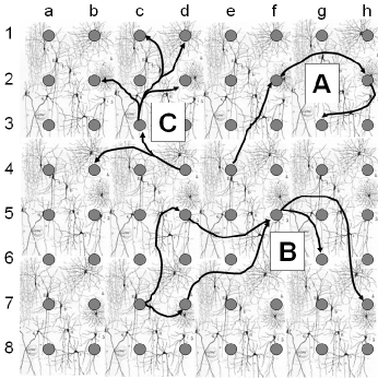
Figure 2: Hypothetical Micro electrode array showing three networks that can manifest as the following episodes: [A]. $\mbox{e4}\rightarrow{\mbox{f2}}\rightarrow{\mbox{h2}}\rightarrow{\mbox{g3}}$, [B]. $\mbox{c7}\rightarrow{\mbox{(d5 d7)}}\rightarrow{\mbox{f5}}\rightarrow{\mbox{(g6 h7)}}$, [C]. $d4\rightarrow{\mbox{(b4 c3)}}\rightarrow{\mbox{(b2 d2 d1 c1)}}$.

Fig. 2 shows (in schematic fashion) how specific neuronal interconnections on a neural tissue underneath a micro electrode array can result in specific temporal patterns (in terms of our episodes) in the spike train data that is obtained from this micro electrode array recordings. In the figure, the electrodes are referred to by their position in the 2D grid and for three different neuronal connection patterns the resulting episode is shown. The connectivity pattern A in the figure gives rise to a serial episode. The other two connectivity patterns give rise to synfire chain type episodes which are a combination of parallel and serial episodes. Thus, when we analyze data obtained through micro electrode array recordings using our algorithms, this is how the episodes are to be interpreted as connectivity patterns.

Summarizing the above discussion, we can say that discovering frequent serial and parallel episodes with appropriate temporal constraints would allow us to identify many of the important patterns in spike train data that capture underlying connectivity information. It is in this aspect that temporal data mining can play a vital role in analyzing spike train data.

4 Discovering frequent episodes under temporal constraints

In this section we describe our algorithms that discover frequent episodes under expiry and inter-event time constraints. Since algorithms for taking care of expiry time are available in case of serial episodes [42], we consider the case of only parallel episodes under expiry time constraint. The inter-event time constraints are meaningful only for serial episodes and that is the case we consider. While describing the details of the algorithm we assume that the reader is familiar with the general structure of frequent episode discovery methods [19, 43]. However, for the sake of readers who are not familiar with these data mining techniques, we also provide some intuitive explanation wherever possible.

A frequent episode is one whose frequency exceeds a user specified threshold. The overall objective is to find all frequent episodes. Counting of all possible episodes is infeasible in most real problems due to combinatorial explosion. As is common in such data mining methods, we use the same basic idea as in level-wise Apriori-style [37] procedure which was first introduced in the context of frequent itemset mining. We briefly explain this idea below.

Consider the problem of discovering all frequent serial episodes up to a given size. The discovery process has two main steps. First, we build a set of candidate episodes and next, we obtain the frequencies (i.e., count the non-overlapping occurrences) of the candidates in the data stream so that we can retain only those whose frequencies are above the user-set threshold. The combinatorial explosion is in candidate generation because the number of possible episodes of a given size increases exponentially with size. For now, let us assume that there are no temporal constraints. The key observation is that an episode can be frequent only if all its subepisodes are frequent. This is obvious because, for example, given two non-overlapping occurrences of $A\rightarrow B\rightarrow C$, we have at least two non-overlapping occurrences of each of its subepisodes. This immediately gives rise to a level-wise procedure for discovering all frequent episodes. First we discover all frequent 1-node episodes. (This is simply a histogram of event types). Then we build a set of candidate 2-node episodes such that the 1-node subepisodes of all candidates are seen to be frequent. Now through one more pass over the data, we count the non-overlapping occurrences of all the candidates and thus come out with frequent 2-node episodes. Now we combine only the frequent 2-node episodes to build a candidate set of 3-node episodes and so on. Thus at stage $n$, using the already discovered set of frequent $n$-node episodes, we build the set of candidate $(n+1)$-node episodes and, by counting their occurrences in the data (using one more pass over the data), we come out with frequent $(n+1)$-node episodes. This procedure controls the combinatorial explosion because we are, after all, interested only in episodes that occur sufficiently often. By choosing a suitable frequency threshold, as the size of episodes grows, the number of frequent episodes would come down. (It is highly unlikely that all large random sequences occur often in the data). Because of this, the number of candidates becomes much less than the combinatorially possible number, as the size of episodes grows. This is the basic idea of Apriori-style procedure used in most frequent pattern mining algorithms.

When we impose temporal constraints, we need to ask whether such a procedure still works. It is easy to see that the property ( referred to as anti monotonicity property) of subepisodes being at least as frequent as the episode holds under expiry time constraint also. This is because every occurrence of the episode that completes within a given (expiry) time would contain occurrences of all the subepisodes which also complete within that time. However this property does not hold under inter-event constraints. Suppose we need the time between any two consecutive events in any serial episode occurrence to be less than, say, $T_{X}$. We may have many occurrences of $A\rightarrow B\rightarrow C$ where each pair of consecutive events occur within time $T_{X}$, but there may be no occurrence of the episode $A\rightarrow C$ such that the time between the two events is less than $T_{X}$. However, as we shall see later on we can still use the level-wise procedure by restricting the check that subepisodes should be frequent, only to certain kind of subepisodes. The idea used here is similar to the concept of ‘loose anti-monotonicity’ in the context of mining frequent itemsets under constraints [12].

Given that we can control the growth of candidates as the size of episodes increases, the next question is how do we count the frequencies of a set of candidate episodes. This is done by having a finite state automaton for each episode such that it recognizes the occurrence of an episode. For example, for a serial episode, $A\rightarrow B\rightarrow C$, there would be an automaton that keeps waiting for an $A$ to transit into its first state and after that, waits for a $B$ to transit into its second state and so on. When this automaton transits into its final state, an occurrence would be complete and then we reset the automaton to wait for an $A$ again. For a parallel episode, conceptually, the states would be subsets of event types in the episode and the current state tells which all event types are yet to occur. We may have to keep track of more than one set of potential state transitions of the automaton and hence we may need multiple automata for each episode in the set of candidates. As we traverse the data, for each event (spike) we encounter, we make appropriate state changes in all the automata (that are waiting for this event type) and whenever an automaton transits to its end state we increment the count of the corresponding episode. Thus, we can simultaneously count the occurrences of a set of candidates using a single pass over the data. Conceptually, all the algorithms for frequent episode discovery use this general framework [19, 43, 40]. We also use the same idea in our algorithms and also use essentially the same data structures as in [43] for keeping track of potential state transitions of different automata. The main data structure is a waits() list which is indexed through event types. That is, waits(A) would store a list of (appropriate representations) of automata that are waiting for an occurrence of $A$. The number of active automata per episode that we need (which is same as the temporary memory needed by the algorithm) depends on what all types of occurrences we want to count. Restricting the count to only non-overlapped occurrences makes the counting process also very efficient [43, 40].

The overall procedure for frequent episode discovery is given below as a pseudo code.

Algorithm 1 Mining Frequent Episodes

1:  Generate an initial set of (1-node) candidate episodes (N=1)

2:  repeat

3:     Count the number of occurrences of the set of (N-node) candidate episodes in one pass of the data sequence

4:     Retain only those episodes whose count is greater than the frequency threshold and declare them to be frequent episodes

5:     Using the set of (N-node) frequent episodes, generate the next set of (N+1-node) candidate episodes

6:  until  There are no candidate episodes remaining

7:  Output all the frequent episodes discovered

When we specify our algorithms in the next two subsections, we explain both candidate generation and frequency counting steps.

4.1 Parallel episodes with expiry

In this section we present an algorithm that counts the number of non-overlapped occurrences of a set of parallel episodes in which all the constituting events occur within time $T_{X}$ of each other. The algorithm here discovers parallel episodes with non-repeated event types. The pseudo-code for the algorithm is listed as Algorithm 2 in the Appendix.

The algorithm takes as input, the set of candidate episodes, the event sequence, the expiry time, $T_{X}$, and the frequency threshold, and outputs the set of frequent episodes. An occurrence of a parallel episodes requires all its constituent nodes to appear in the event sequence in any order. At any given time, one needs to wait for all the nodes of the episode that remain to be seen. In the implementation of the algorithm here, instead of a single automaton waiting for a set of event types, we maintain separate entries for each distinct event type of the episode using a $waits(.)$ list indexed by event types. For event type $A$, each entry in the list $waits(A)$ is of the form $(\alpha,count,init)$, where $\alpha$ is an episode waiting for an $A$, “$count$” takes values 1 or 0 depending on whether an event of this type ($A$) has been seen or not, and $init$ indicates the latest time of occurrence of this event type. The Algorithm 2, given as pseudo code, specifies the details of how the $waits$ list is updated as we traverse the data.

An occurrence of an episode is complete when all required event types have been encountered at least once and all the event times (remembered by $init$ field) occur within $T_{X}$ of each other. An episode specific $counter$ is used to keep track of the event types already seen. When an occurrence is complete, the episode frequency count is incremented and all the entries (in the $waits(.)$ lists) for the episode are reinitialized.

If the expiry check fails, we cannot reject all the events types of the partial occurrence. This is because, in an occurrence of a parallel episode, the constituent event types can occur in any order in the event stream. Only those event types which have occurred before $(t_{i}-T_{X})$, should be rejected, where $t_{i}$ is the time of the latest event type seen by the algorithm. Effectively, any later occurrence of these events could possibly complete the parallel episode (without violating the temporal constraint).

Candidate generation

The candidate generation scheme is very similar to the one presented in [37] for itemsets. Let $\alpha$ and $\beta$ be two $k$-node frequent episodes having first $(k-1)$ nodes identical. The potential $(k+1)$-node candidate is generated by appending to $\alpha$ the $k^{th}$node of $\beta$. This new episode is declared as a $(k+1)$-node candidate if all its $k$-node subepisodes are already known to be frequent.

4.2 Serial Episodes with Inter-event Constraints

Under an inter-event time constraint, the time difference between successive events in any occurrence have to be in a prescribed interval. The episode structure now consists of an ordered set of intervals besides the ordered set of event types. For example, a 4-node serial episode is now denoted as follows:

$$(A^{\underrightarrow{(t_{low}^{1},t_{high}^{1}]}}B^{\underrightarrow{(t_{low}^{2},t_{high}^{2}]}}C^{\underrightarrow{(t_{low}^{3},t_{high}^{3}]}}D)$$ (2)

In a given occurrence of episode $A\rightarrow$ $B\rightarrow$ $C\rightarrow$ $D$ let $t_{A}$, $t_{B}$, $t_{C}$ and $t_{D}$ denote the time of occurrence of corresponding event types. Then this is a valid occurrence of the serial episode with inter-event time constraint given by (2), if $t_{low}^{1}$ $<$ $(t_{B}-t_{A})$ $\leq$ $t_{high}^{1}$, $t_{low}^{2}$ $<$ $(t_{C}-t_{B})$ $\leq$ $t_{high}^{2}$ and $t_{low}^{3}$ $<$ $(t_{D}-t_{C})$ $\leq$ $t_{high}^{3}$.

In general, an $N$-node serial episode is associated with, $N-1$ inter-event constraints of the form $(t_{low}^{i},t_{high}^{i}]$. The algorithm we present is for generalized inter-event constraints. The user needs to specify only the granularity of search by providing a set of non-overlapped time intervals to serve as candidate inter-event time intervals. The algorithm discovers all frequent episodes along with the choice of most appropriate inter-event intervals for each episode.

4.2.1 Candidate generation scheme

As explained earlier, when we have inter-event time constraints, it is not necessary that all subepisodes have to be frequent for an episode to be frequent. In the data sequence, if episode $(A^{\underrightarrow{(0,5]}}$ $B^{\underrightarrow{(5,10]}}$ $C)$ is frequent, the sub-episodes $(A^{\underrightarrow{(0,5]}}$ $B)$ and $(B^{\underrightarrow{(5,10]}}$ $C)$ are also as frequent, but pairing event type $A$ with $C$ we would get $(A^{\underrightarrow{(?,?]}}$ $C)$ as a subepisode whose inter-event constraint is not intuitive.

The candidate episodes in this case are generated as follows. Let $\alpha$ and $\beta$ be two $k$-node frequent episodes such that by dropping the first node of $\alpha$ and the last node of $\beta$, we get exactly the same $(k-1)$-node episode. That is, the $(k-1)$-event types match and also the $(k-2)$-intervals corresponding to the inter-event constraints match. A candidate episode $\gamma$ is generated by copying the $k$-event types and $(k-1)$-intervals of $\alpha$ into $\gamma$ and then copying the last event type of $\beta$ into the $(k+1)^{th}$ event type of $\gamma$ and the last interval of $\beta$ to the $k^{th}$ interval of $\gamma$. Fig. 3 shows the candidate generation process graphically.

Figure 3: Visualization of Candidate generation for serial episodes with inter-event constraints

It is easy to see that, under inter-event time constraints, an episode cannot be frequent unless such prefix and suffix subepisodes are frequent. It is this necessary condition that our candidate generation scheme exploits. This method of candidate generation is very similar to the ones used in case of mining of sequential patterns under similar inter-event constraints [45, 32].

4.2.2 Counting episodes with generalized inter-event time constraint

As already stated, the constraints are in the form of intervals $(t_{low}^{i},t_{high}^{i}]$, in which the inter-event times must lie. We first explain the difficulty in taking care of such constraints under the currently available algorithms for counting maximum number of non-overlapped occurrences of serial episodes.

Suppose we want to count the non-overlapped occurrences of $A\rightarrow B\rightarrow C\rightarrow D$. In the data sequences there may be many instances of $A$, $B$, and $C$ before we get the first $D$ and the method of counting has to decide which of these to take while scanning the data from left to right for constituting an occurrence. There are two distinguishable approaches here which were used. Given a set of overlapped occurrences of the episode all ending on the same event, the one which starts earliest is called the left-most occurrence and the one that starts last is called the inner-most occurrence. (See [42] for more discussion). Consider the event sequence

$$\langle(A,1),(A,2),(B,4),(A,5),(C,10),(B,12),(C,13),(D,17)\rangle.$$ (3)

This contains exactly one non-overlapped occurrence of the four node episode. Here, the left-most occurrence is $\langle(A,1),$ $(B,4),$ $(C,10),$ $(D,17)\rangle$ and the inner-most occurrence is $\langle(A,5),$ $(B,12),$ $(C,13),$ $(D,17)\rangle$. Counting the left-most occurrence is efficient because we make a transition as soon one can be made and we do not need to remember any other possible transitions. On the other hand, for counting the inner-most occurrence we have to remember multiple transition possibilities. However, for implementing expiry time constraint, we have to count the inner-most occurrence because the left-most occurrence may not satisfy the expiry time constraint. (If any of the occurrences in this set of occurrences satisfy the expiry time constraint then the inner-most would). There are algorithms for counting non-overlapped occurrences of serial episodes in both these fashions. When we have inter-event constraints, we can not get maximum number of non-overlapped occurrences by counting only either left-most or inner-most. Suppose, in this example, the inter-event constraints are given as $(A^{\underrightarrow{(0,5]}}$ $B^{\underrightarrow{(5,10]}}$ $C^{\underrightarrow{(0,5]}}$ $D)$. In the given event sequence, only the occurrence $\langle(A,2),$ $(B,4),$ $(C,13),$ $(D,17)\rangle$ satisfies the inter-event interval constraints. This is the reason we need to modify the counting scheme so as to remember more number of potential transitions than needed to count inner-most occurrences.

The counting algorithm is listed as Algorithm 2 in the Appendix. The algorithm presented uses $waits$ lists indexed by event types as the basic data-structure. The entries in the $waits$ lists are structures called $node$s. For each episode we have a doubly linked list of $node$ structures with a $node$ corresponding to each of the event types and arranged in the same order as that of the episode. The $node$ structure has a $tlist$ field that stores the times of occurrence of the event-type represented by its corresponding $node$. For example, in the event sequence given by (3), the $node$ representing $A$, after $t=5$, would have $tlist=\{(A,1),(A,2),(A,5)\}$. Other field in the $node$ structure is $visited$, which is a boolean field that indicates whether the event type is seen at least once.

On seeing an event type $E_{i}$, the algorithm iterates over list $waits(E_{i})$ and updates each $node$ in the list. We explain the procedure for updating the $node$s by considering the the example sequence given in (3) and the episode $\alpha=(A^{\underrightarrow{(0,5]}}$ $B^{\underrightarrow{(5,10]}}$ $C^{\underrightarrow{(0,5]}}$ $D)$. Working of the algorithm in this example is illustrated in Fig. 4.

The $waits$ lists are initialized by adding the $node$s corresponding to first event type of each episode in the set of candidates to the corresponding $waits(.)$ list. In the example, let the $node$ tracking event type $A$ be denoted by $node_{A}$, and so on. Initially $waits(A)$ contains $node_{A}$. The boxes in Fig. 4 represent an entry in the $tlist$ of a $node$. An empty box is one that is waiting for the first occurrence of an event type. On seeing $(A,1)$, it is added to $tlist$ of $node_{A}$, and $node_{B}$ is added to $waits(B)$. At any time, the $node$ structures are waiting for all event types that have been already seen and the next unseen event type.

The algorithm is now waiting for an occurrence of a $B$ and an $A$ as well. At $t=4$, the first occurrence of a $B$ is seen. The $tlist$ of $node_{A}$ is traversed to find at least one occurrence of $A$, such that $t_{B}-t_{A}\in(0,5]$. Both $(A,1)$ and $(A,2)$ satisfy the inter-event constraint and hence, $(B,4)$ is accepted into the $node_{B}.tlist$. The rule for accepting an occurrence of an event type (which is not the first event type of the episode) is that there must be at least one occurrence of the previous event type (in this example $A$) which can be paired with the occurrence of the current event type (in this example $B$) without violating the inter-event constraint. After seeing the first occurrence of $B$, $node_{C}$ is added to $waits(C)$. Using the above rules the algorithms accepts $(A,5)$, $(C,10)$ into the corresponding $tlist$s. At $t=12$, for $(B,12)$ none of the entries in $node_{A}.tlist$ satisfy the inter-event constraint for the pair $A\rightarrow B$. Hence $(B,12)$ is not added to the $tlist$ of $node_{B}$. Rest of the steps of the algorithm are illustrated in the figure.

If an occurrence of event type is added to $node.tlist$, it is because there exist events for each event type from the first to the event type corresponding to the $node$, which satisfy the respective inter-event time constraints. An occurrence of episode is complete when an occurrence of the last event type can be added to the $tlist$ of the last $node$ structure of the episode.

The $tlist$ entries shown crossed out in the figure are the ones that can be deallocated from the memory. In the example, at $t=12$, when the algorithm tries to insert $(B,12)$ into $node_{B}.tlist$, the list of $tlist$ entries for occurrences of $A$ is traversed. $(A,1)$ with inter-event constraint $(0,5]$ can no longer be paired with a $B$ since the inter-event time duration for any incoming event exceeds $5$, hence $(A,1)$ can be safely removed from the $node_{A}.tlist$. This holds for $(A,2)$ and $(A,5)$ as well. In this way the algorithm frees memory wherever possible without additional processing burden.

In order to track episode occurrences we need to store sufficient back references in data structures to back track each occurrence. This adds some memory overhead, but tracking may be useful in visualizing the discovered episodes.

Figure 4: Visualization of Algorithm 3

5 Simulation Results

In this section we present some results obtained with our algorithms for analyzing spike-train data. We mainly discuss results obtained on synthetic data generated through a simulation model. We also present some results on data gathered from experiments on neural cultures. The main reason for using simulator-generated data is that here we can have control on the kind of patterns that the data contains and can thus check whether our algorithms discover the ‘true’ patterns. Also, by generating many sets of random data we can study the statistical properties of the algorithms. The simulation model is intended to generate fairly realistic spike trains. For this we simulate a network of neurons where each neuron is modeled as an inhomogeneous Poisson process whose rate changes with the input received by the neuron. On simulator-generated data we present results to show that our algorithms can discover different types of embedded patterns. We also present some empirical results to argue that the patterns discovered would be statistically significant.

5.1 The spike data generation model

For the data generation, we use a simulator where each neuron is modeled as an inhomogeneous poisson process. The neurons are interconnected and there is a weight attached to each interconnection or synapse. The rate of firing of each neuron is time-varying and it is dependent on the weighted sum of spikes received (over a time window) as input by the neuron from the others through the synapses. The rate is updated every $\Delta T$ time units. We use two different functions to change the firing rate of a neuron in response to inputs received and test our methods in both scenarios.

As explained earlier, the intuitive reason why temporal data mining may be effective for spike data analysis is the following. Suppose neuron $A$ is connected to $B$ and the neuron $B$ to $C$ through excitatory synapses each of synaptic delay of about $T$. When $A$ fires, because of the excitatory synapse, the firing rate of $B$ would go up after a delay of about $T$ and similarly for the $B$ to $C$ connection. Then, irrespective of the underlying mechanism of changing the rate as a function of input, we would essentially have high conditional probability of seeing a spike from $B$ at time $T$ given $A$ has spiked at time zero and similarly for the $B$ to $C$ connection. This would make an occurrence of the serial episode, $A\rightarrow B\rightarrow C$ with inter-event constraint of about $T$, much more likely than that for any other triplet of non-interconnected neurons. Thus if a 3-node episode like this has high enough frequency (in terms of number of non-overlapped occurrences) then it is very likely that it indicates such a connectivity pattern. As long as the underlying model of interconnected neurons results in a high value of the conditional probability referred to above, the data mining technique would be able to discover the connectivity pattern irrespective of the specific underlying mechanism of interaction among neurons. (Note that if we postulate a specific stochastic model for the interacting neurons and then estimate the model parameters, the analysis results are tightly coupled with the assumed model). It is simply to illustrate this that we have used two different ways of updating the rate of firing based on the input. The specific mechanisms may or may not be biologically plausible; but are used here to demonstrate model independence of the proposed technique.

The two methods of updating the firing rate are as follows. The first one uses a sigmoidal relationship. Specifically we use

$$\lambda_{j}(k)=\frac{\lambda_{1j}}{1+\exp{(-I_{j}(k)+d)}}$$ (4)

where $\lambda_{j}(k)$ is the firing rate of $j^{th}$ neuron at time $k\Delta T$ and $I_{j}(k)$ is its total input at that time. $I_{j}(k)=\sum_{i}O_{i}(k)w_{ij}$ where $O_{i}(k)$ is the output of $i^{th}$ neuron (as seen by the $j^{th}$ neuron) at time $k\Delta T$ and $w_{ij}$ is the weight of synapse from $i^{th}$ to $j^{th}$ neuron. $O_{i}(k)$ is taken to be the number of spikes by the $i^{th}$ neuron in the time interval $(\;(k-h-1)\Delta T,\ (k-h)\Delta T]$ where $h$ represents the synaptic delay in units of $\Delta T$. The offset parameter $d$ determines the resting spiking rate $\lambda_{0j}$ (i.e. the firing rate when input is zero). This is the quiescent firing rate (or the noise level) in the system. We choose $\lambda_{1j}$ to ensure that we reach the desired high firing rate on receiving the amount of input that should prime this neuron to fire. An absolute refractory period is also implemented. This is the short time after a spike in which the neuron cannot respond to another stimulus.

In the second method of updating, the firing rate is low if input is low and increases linearly with input till it reaches the desired firing rate for full input and saturates at that rate. Specifically we use

$$\lambda_{j}(k) = 0\ \ \mbox{~{}if~{}}\ I_{j}(k)\leq-\frac{\lambda_{0j}}{a}$$ (5)

$$= aI_{j}(k)+\lambda_{0j}\ \ \mbox{~{}if~{}}\ -\frac{\lambda_{0j}}{a}\leq I_{j}(k)\leq I_{1j}$$

$$= \lambda_{1j}\ \ \mbox{~{}if~{}}\ I_{j}(k)>I_{1j}$$

Here, $a$ is a suitable constant that determines slope of the linear region, $\lambda_{0j}$ represents the quiescent firing rate of neuron $j$ which is the firing rate when input is zero and $\lambda_{1j}$ represents the high firing rate which is reached on full input (which is represented by the parameter, $I_{1j}$). The input to the $j^{th}$ neuron at time $k\Delta T$, $I_{j}(k)$, is determined as in the earlier case.

To employ either model, in the simulator we specify the quiescent rate of firing (denoted by $\lambda_{0}$) and the required conditional probability of the receiving neuron firing (denoted by $\rho$) when it receives the full expected input. The quiescent firing rate determines $d$ in the first model and $\lambda_{0j}$ in the second model. The conditional probability specified determines the high end of firing rate we want to reach. Now we choose the weight values for the intended connections so that on receiving the full input we reach the high firing rate needed to satisfy the specified conditional probability.

We use these models to generate data with different patterns as follows. Let N denote the total number of neurons in the system. (We have generated data with N=26, 64 and 100). First we randomly interconnect the neurons. For each neuron we randomly choose $M$ other neurons to interconnect it with. (We used $M=N/2$ and $N/4$). The weight attached to each synapse is set randomly using a uniform distribution over $[-c,\;c]$.. When we want to embed any specific pattern, then, we set the weights of the required connections between neurons to a higher value. The weight value depends on the type of pattern to be embedded. The patterns we want to embed are the kind shown in Fig. 1. These are realizable by essentially two types of pattern dependent interconnections between neurons. One is where a neuron primes one (as in a serial episode) or many (as in a parallel episode) neurons. Here a high conditional probability ($\rho$) is assigned to each interconnection that forms the part of a pattern and the corresponding weight is determined by requiring that one spike (in the appropriate interval) by the priming neuron would increase the firing rate of the receiving neuron so that in the next $\Delta T$ interval (after the synaptic delay time) the receiving neuron spikes at least once with probability $\rho$. (The required firing rate is determined based on $\rho$). The other kind of interconnection is where many neurons together prime one neuron (which is used in Synfire chains). Here, the weight of each connection is set in such a way that only if each of the input neurons spikes once in the appropriate interval then the firing rate of the receiving neurons would go up to the high value. (If only a few of the input neurons fire, then the firing rate of the receiving neuron goes up but not all the way up to the high level).

The simulator runs as follows. At any given time, we have some spiking rates for all the neurons. Using this, spikes are generated (as a Poisson process) for the next $\Delta T$ time interval for every neuron. (Since we are using a Poisson process model, the time of a spike would be a real number). Then, using the spiking history, we calculate the inputs into each neuron and update the spiking rate for each neuron using eq.(4) or (5) depending on which model we are using. Then with the new spiking rates we generate spikes from every neuron for the next $\Delta T$ and so on. We also implement an absolute refractory period for each neuron. Once the spikes are generated for a $\Delta T$ interval, starting with the second spike we remove spikes one by one if they are closer than $\tau_{r}$ to the previous spike where $\tau_{r}$ is the refractory time.

The network contains both random interconnections among neurons as well as interconnections (with larger weights) that together constitute some patterns embedded. The weights of random connections are set using a mean-zero distribution and hence, in an expected sense all neurons keep firing at the ‘noise’ rate of $\lambda_{0}$. However, since the actual input can still assume small positive and negative values, this background firing rate would also be fluctuating around $\lambda_{0}$. Since all firings are stochastic, even when a pattern is embedded, the entire patterned firing sequence will not always happen. Also, within a pattern of firing of neurons (as per the embedded pattern), there would be other neurons that would be spiking randomly. Though we calculate the input into neurons and their firing rates at only discrete time points (separated by $\Delta T$), since each neuron’s spikes are (inhomogeneous) Poisson, the actual times of spikes would be continuous. That is, the time of spikes would not be integral multiples of $\Delta T$. ( We note in passing that, due to our implementing of refractory period, the actual firings of neurons are not strictly Poisson).

For the simulations discussed here, we generally use the following values for parameters: $\lambda_{0}=20Hz$, $\rho=0.95$. We have chosen $\Delta T=1$ ms and chosen the refractory period ($\tau_{r}$) also the same. (This would mean that in any $\Delta T$ interval there would be at most one spike from any neuron). For calculation of input into a neuron, we mostly use $h=5$ which implies a synaptic delay of 5 ms. In some examples, where we want to choose different synaptic delays for different connections we change the value of $h$ as needed. Similarly we can use different $\lambda_{0}$ for different neurons and different $\rho$ for different patterned interconnections when needed.

5.2 Discovering Network patterns

In this section, we demonstrate how we can obtain useful information about the structure of the underlying network using combination of serial and parallel episode discovery. Using the simulation model described above, we can embed different types of network patterns. Fig.1 shows examples of types of inter connections we make to embed different patterns. For this, in the simulator we make these required connections between neurons have high weights as explained in the previous subsection. (In addition there are also random interconnections among neurons).

We discuss three examples to illustrate that our method is very effective in unearthing the underlying connectivity pattern. For each example we use a specific connectivity pattern and generate spike data using our simulator with these embedded patterns. We then use our algorithms to discover frequent parallel and serial episodes with different temporal constraints. As explained earlier, synchronous firing patterns are well captured by parallel episodes with appropriate expiry time constraint, ordered firing patterns are captured by serial episodes with inter-event constraints and synfire chains are captured by a combination of parallel and serial episodes. We illustrate all this in the examples.

Example 1

Figure 5: Network pattern for Example 1

In a 26 neurons network (where each neuron corresponds to an alphabet) we embed the pattern shown in Fig.5. The simulation is run for 50 seconds. (In this time approximately 25,000 spikes are generated when we use eq. (4) and about 20,000 spikes are generated when we use eq. (5) ). The synaptic delay is set to 5 ms. We have chosen $\Delta T=1$ ms and have taken refractory time also to be the same.

Episode	Freq.	Time	Size	Patterns
expiry	Th.	(sec)	(No.)	Discovered
0.0001	0.01	0.23	1(26)	no episode of 2
				or more nodes
0.001	0.01	0.29	2(2)	E C : 799; F D : 624
0.002	0.01	0.28	2(2)	E C : 804; F D : 643
0.007	0.01	0.37	4(1)	F E D C : 615

Table 1: Parallel episodes for Example 1. The data is generated using (4) for updating firing rate of neurons

Episode	Freq.	Time	Size	Patterns
expiry	Th.	(sec)	(No.)	Discovered
0.0001	0.01	0.23	1(26)	no episode of 2
				or more nodes
0.001	0.01	0.25	2(2)	E C : 652; F D : 502
0.002	0.01	0.17	2(2)	E C : 683; F D : 603
0.007	0.01	0.48	4(1)	F E D C : 525

Table 2: Parallel episodes for Example 1. The data is generated using (5) for updating firing rate of neurons.

Inter-event	Freq.	Time	Size	Patterns
interval	Th.	(sec)	(No.)	Discovered
0.000-0.001	0.01	0.29	2(4)	C E : 410; E C : 400
				D F : 329; F D : 303
0.000-0.002	0.01	0.31	2(4)	C E : 422; E C : 408
				D F : 348; F D : 323
0.002-0.004	0.01	0.26	1(26)	no 2 or more
				node episodes
0.004-0.006	0.01	0.29	4(4)	A B C D : 597
				A B E F : 589
				A B E D : 530
				A B C F : 530

Table 3: Serial episodes for Example 1. The data is generated using (4) for updating firing rate of neurons

Inter-event	Freq.	Time	Size	Patterns
interval	Th.	(sec)	(No.)	Discovered
0.000-0.001	0.01	0.27	2(4)	C E : 350; E C : 321
				D F : 254; F D : 263
0.000-0.002	0.01	0.31	2(4)	C E : 382; E C : 365
				D F : 330; F D : 338
0.002-0.004	0.01	0.26	1(26)	no 2 or more
				node episodes
0.004-0.006	0.01	0.29	4(4)	A B C D : 259
				A B E F : 248
				A B E D : 220
				A B C F : 213

Table 4: Serial episodes for Example 1. The data is generated using (5) for updating firing rate of neurons

The sequence is then mined for frequent parallel episodes with different expiry times. The results are given in Tables 1 and 2 for the two cases of data generated with models (4) and (5). The tables show the expiry time used, the frequency threshold, time taken by the algorithm on a Intel dual core PC running at 1.6 GHz, the size of the largest frequent episode discovered and the number of episodes of this size along with the actual episodes and their frequencies. (In the tables, all times are shown in seconds). We follow the same structure for all the tables. The frequency threshold is expressed as a fraction of the entire data length. A threshold of 0.01 over a data length of 25,000 spike events requires an episode to occur at least 250 times before it is declared as frequent. In the algorithm, this frequency threshold is what is used for episodes of size 1. As the size of episodes increases, the expected frequency decreases and hence we should suitably decrease the threshold. (See [43] for a more precise account of this). Hence, we reduce the frequency threshold by a factor of 0.9 for each successively larger size of episodes. From Table 1 it can be seen that $(CE)$ and $(DF)$ turn out to be the only frequent parallel episodes if the expiry time is 1 to 2 ms. If the expiry time is too small (less than 1 ms), we get no frequent episodes. On the other hand, if we increase the expiry time to be 7 ms which is greater than a synaptic delay, then even $(FEDC)$ turns out to be a parallel episode. From Table 2, it can be seen that the results obtained are the same even when we use the linear model given by (5) for changing the firing rates of neurons. The only difference is some minor variation in the actual number of non-overlapped occurrences. As long as the frequency is high enough the actual number is unimportant in discovering frequent episodes. These results show that by using appropriate expiry time, parallel episodes discovered capture connectivity structure representing synchronous firing patterns.

The results of serial episode discovery are shown in Tables 3 and 4 for the two models of updating firing rates of neurons. With an inter-event constraint of 4-6 ms, we discover all paths in the network (Fig. 5). When we prescribe that inter-event time be less than 2 ms (while synaptic delay is 5 ms), we get nodes in the same level as our serial episodes. If we use intervals of 2-4 ms, we get no episodes because synchronous firings mostly occur much closer and firings related by a synapse have a delay of 5 ms. Thus, using inter-event time constraints, we can get fair amount of information of the underlying connection structure that contributes to ordered firings. It may seem surprising that we also discover $A\rightarrow B$ $\rightarrow C$ $\rightarrow F$ and $A\rightarrow B$ $\rightarrow E$ $\rightarrow D$ when we use 4–6 ms constraint. This is because, the network structure is such that $D$ and $F$ fire about one synaptic delay time after the firing of $C$ and $E$. Thus, the serial episodes give the sequential structure in the firings which could, of course, be generated by different interconnections. The frequent episodes discovered provide a handle to unearthing the hierarchy seen in the data (i.e. which events co-occur and which ones follow one another). As seen from the tables, we get similar results with both methods of updating the firing rate.

Example 2

In this example we consider the network connectivity pattern as shown in Fig. 1(c). As stated earlier, this is an example of possible network connectivity that can generate patterns known as Synfire chains. We use the same parameters in the simulator as in Example 1 and generate spike trains data using this connectivity pattern. As earlier, we generate data sets using the two different models for updating firing rates. Tables 5 and 6 show the parallel episodes discovered and Tables 7 and 8 show the serial episodes discovered under the two methods of updating firing rates. From the tables, it is easily seen that parallel episodes with expiry time of 1 ms and serial episodes with inter-event time constraint of about one synaptic delay, together give good information about underlying network structure. Since the synaptic delay is taken to be 5ms, when we use an inter-event time constraint of 4–6ms, all paths in the network become frequent serial episodes. There are 24 such serial episodes and hence the tables list only a few. Once again, the results under the two models of updating firing rates, are identical.

In this example, we illustrate how our algorithms can discover synfire chain patterns. We first discover all parallel episodes with expiry time 1 ms. Then for each frequent parallel episode, we replace each of its occurrences in the data stream by a new event with event type being the name of the parallel episode. This new event is put in with a time of occurrence which is the mean time in the episode occurrence. We then discover all serial episodes with different inter-event time constraints. The results obtained with this method are shown in Tables 9 and 10. As can be seen, the only pattern we discover is the underlying synfire chain. (In the tables, the size of this is shown as the size of the serial episode where some of the nodes may be parallel episodes). This example shows that by proper combination of parallel and serial episodes, we can obtain fairly rich pattern structures which are of interest in neuronal spike train analysis.

Episode	Freq.	Time	Size	Patterns
expiry	Th.	(sec)	(No.)	Discovered
0.001	0.01	0.15	4(1)	L K : 307
				C B D : 293
				H G F I : 268
				rest are
				sub-episodes

Table 5: Parallel episodes for Example 2. The data is generated using (4) for updating firing rate of neurons

Episode	Freq.	Time	Size	Patterns
expiry	Th.	(sec)	(No.)	Discovered
0.001	0.01	0.1	4(1)	L K : 228
				C B D : 204
				H G F I : 195
				rest are
				sub-episodes

Table 6: Parallel episodes for Example 2. The data is generated using (5) for updating firing rate of neurons.

Inter-event	Freq.	Time	Size	Patterns
interval	Th.	(sec)	(No.)	Discovered
0.002-0.004	0.01	0.16	1(26)	no episodes of 2
				or more nodes
0.004-0.006	0.01	0.47	6(24)	A D E H J K : 195
				A D E I J K : 194
				A D E H J L : 193
				A C E H J K : 192
0.006-0.008	0.01	0.16	1(26)	no episodes of 2
				or more nodes

Table 7: Serial episodes for Example 2. The data is generated using (4) for updating firing rate of neurons

Inter-event	Freq.	Time	Size	Patterns
interval	Th.	(sec)	(No.)	Discovered
0.002-0.004	0.01	0.19	1(26)	no episodes of 2
				or more nodes
0.004-0.006	0.01	0.35	6(24)	A D E H J K : 145
				A D E I J K : 134
				A D E H J L : 132
				A C E H J K : 121
0.006-0.008	0.01	0.1	1(26)	no episodes of 2
				or more nodes

Table 8: Serial episodes for Example 2. The data is generated using (5) for updating firing rate of neurons

Inter-event	Freq.	Time	Size	Patterns
interval	Th.	(sec)	(No.)	Discovered
0.002-0.004	0.01	0.11	1(20)	no episodes of
				2 or more nodes
0.004-0.006	0.01	0.14	6(1)	A [C B D] E
				[H G F I] J [L K] : 137
0.006-0.008	0.01	0.12	1(20)	no episodes of
				2 or more nodes

Table 9: Synfire episodes for Example 2. The data is generated using (4) for updating firing rate of neurons

Inter-event	Freq.	Time	Size	Patterns
interval	Th.	(sec)	(No.)	Discovered
0.002-0.004	0.01	0.2	1(20)	no episodes of
				2 or more nodes
0.004-0.006	0.01	0.3	6(1)	A [C B D] E
				[H G F I] J [L K] : 108
0.006-0.008	0.01	0.1	1(20)	no episodes of
				2 or more nodes

Table 10: Synfire episodes for Example 2. The data is generated using (5) for updating firing rate of neurons

Example 3

In this example, we choose a network pattern where different pairs of interconnected neurons can have different synaptic delays and we demonstrate the ability of our algorithm to automatically choose appropriate inter-event intervals. The pattern is shown in Fig. 6, where we have different synaptic delays as indicated on the figure, for different inter-connections.

Figure 6: Network Pattern for Example 3

Episode	Freq.	Time	Size	Patterns
expiry	Th.	(sec)	(No.)	Discovered
0.001	0.01	0.28	3(1)	A B C : 614
0.002	0.01	0.25	3(1)	A B C : 617
0.004	0.01	0.28	4(1)	A B C D : 537
0.006	0.01	0.32	4(2)	X A B C : 602
				A B C D : 542

Table 11: Parallel episodes for Example 3. The data is generated using (4) for updating firing rate of neurons

Episode	Freq.	Time	Size	Patterns
expiry	Th.	(sec)	(No.)	Discovered
0.001	0.01	0.3	3(1)	A B C : 492
0.002	0.01	0.35	3(1)	A B C : 505
0.004	0.01	0.3	4(1)	A B C D : 431
0.006	0.01	0.32	4(2)	X A B C : 449
				A B C D : 439

Table 12: Parallel episodes for Example 3. The data is generated using (5) for updating firing rate of neurons

Inter-event	Freq.	Time	Size	Patterns
interval	Th.	(sec)	(No.)	Discovered
0.000-0.002	0.01	0.32	2(6)	A C : 385; B A : 376
				B C : 373; A B : 372
				C A : 361; C B : 355
0.002-0.004	0.01	0.37	2(4)	E F : 783; A D : 656
				C D : 651; B D : 646
0.004-0.006	0.01	0.28	2(3)	X A : 790; X B : 774
				X C : 769
0.006-0.008	0.01	0.29	2(2)	D E : 720; X D : 454

Table 13: Serial Episodes for Example 3. The data is generated using (4) for updating firing rate of neurons

Inter-event	Freq.	Time	Size	Patterns
interval	Th.	(sec)	(No.)	Discovered
0.000-0.002	0.01	0.35	2(6)	A C : 301; B A : 297
				B C : 271; A B : 262
				C A : 261; C B : 254
0.002-0.004	0.01	0.41	2(4)	E F : 584; A D : 566
				C D : 551; B D : 562
0.004-0.006	0.01	0.25	2(3)	X A : 602; X B : 598
				X C : 627
0.006-0.008	0.01	0.35	2(2)	D E : 554; X D : 202

Table 14: Serial Episodes for Example 3. The data is generated using (5) for updating firing rate of neurons

Inter-event	Freq.	Time	Size	Patterns
interval	Th.	(sec)	(No.)	Discovered
{0.000-0.002,	0.01	1.37	5(1)
0.002-0.004,				$X^{\underrightarrow{0.004-0.006}}[ABC]$
0.004-0.006,				${}^{\underrightarrow{0.002-0.004}}D^{\underrightarrow{0.006-0.008}}$
0.006-0.008,				$E^{\underrightarrow{0.002-0.004}}F$ : 372
0.008-0.010}

Table 15: Synfire episodes for Example 3. The data is generated using (4) for updating firing rate of neurons

Inter-event	Freq.	Time	Size	Patterns
interval	Th.	(sec)	(No.)	Discovered
{0.000-0.002,	0.01	2.1	5(1)
0.002-0.004,				$X^{\underrightarrow{0.004-0.006}}[ABC]$
0.004-0.006,				${}^{\underrightarrow{0.002-0.004}}D^{\underrightarrow{0.006-0.008}}$
0.006-0.008,				$E^{\underrightarrow{0.002-0.004}}F$ : 287
0.008-0.010}

Table 16: Synfire episodes for Example 3. The data is generated using (5) for updating firing rate of neurons

The results for parallel episode discovery (see Tables 11 and 12) show that $(ABC)$ is the group of neurons that co-spike together. The serial episode discovery results are given in Tables 13 and 14. As can be seen from the table, with different pre-specified inter-event time constraints we can discover only different parts of the underlying network graph because no single inter-event constraint captures the full pattern.

As in Example 2, we replace occurrences of parallel episode with a new event in the data stream. We then run Algorithm 3 to discover serial episodes along with inter-event constraints, given a set of possible inter-event intervals. The results obtained are shown in Tables 15 and 16. As can be seen from the table, we can discover correctly the underlying network pattern. This example illustrates our algorithm for choosing inter-event constraints automatically. Given a set of possible intervals, the algorithm has been able to correctly identify the different synaptic delays in the network pattern. As in the other two examples, we get the same results in terms of frequent episodes irrespective of the method used to update the firing rates of neurons.

The examples presented in this subsection illustrate the effectiveness of our temporal data mining method in inferring useful information regarding connectivity patterns. Here we have presented the case where only one connectivity pattern is embedded. We have tested the algorithm with multiple such patterns also. We have used up to four different patterns of varying lengths all embedded together and the algorithms are found to be effective in inferring all the connectivity patterns. (See [9, 23] for details of these results).

5.2.1 Assessing significance of discovered patterns

The examples above show that if we generate spike data using special embedded patterns in it then our algorithms can detect them. However, this does not answer the question: if the algorithm detects some frequent episodes what confidence do we have that they correspond to some patterns. This essentially concerns the statistical significance of the discovered episodes.

To answer this question we have to essentially choose a null hypothesis that asserts that there is no ‘structure’ in the system generating the data. Then we need to calculate the probability that an episode of a given size would have a given frequency (that is, number of non-overlapped occurrences) in the data generated by such a model and this will tell us what is the chance of a discovered frequent episode coming up by chance in ‘random’ data and hence tells us the statistical significance of the discovered frequent episodes. This can also allow us to calculate the frequency threshold so that all frequent episodes (with frequency above this threshold) are statistically significant at a given level of confidence. We are currently developing appropriate statistical models for such a null hypothesis to derive the required confidence bounds and would be discussing them in our future work. For this paper, we present empirical results to show that long episodes with high frequency do not come up unless the data contains specific biases for coordinated firing by neurons.

Currently, in all reported methods of spike data analysis, whenever issues of statistical significance are considered, it is always with a null hypothesis of iid processes generating spike data.. However, we would like a null hypothesis that says there is no strong structure in the interactions among neurons. Being able to reject a null hypothesis of iid processes generating data, does not seem appropriate when we want to assert that the patterns we found denote strong interactions among neurons. Hence, we want to consider a composite null hypothesis in which we include not only iid processes, but also other models for interdependent neurons without any specific strong connectivity patterns or strong predispositions for coordinated firing. Due to difficulties with analytical tractability, instead of an analytical approach, we take the empirical approach of capturing our null hypothesis in a simulation model and estimate the relevant probabilities by generating many random data sets from such a model. (This approach is similar in spirit to the so called ‘jitter’ method [2]).

We generate our random data sets using essentially three different types of models. For the first one, we use the same simulator as described earlier; but we allow only the random interconnections. (The weights of interconnections would be uniformly distributed over a range that represents small values for the conditional probability of the receiving neuron firing given that the sending neuron has generated a spike). Next, we generate data sets by assuming that different neurons generate spikes as independent Poisson processes by simply choosing random fixed rates for the neurons. In this, we also include cases where many neurons can have the same firing rate. For this, we fix five or ten different random firing rates and randomly assign each neuron to have one of these firing rates. For our third type of data sets, we include models where rates of firing by neurons change; but without any relation to firing by other neurons. For this we choose random firing rates for neurons and at $\Delta T$ time steps we randomly change the firing rate. Here also we include the case where firing rates of some random subsets of neurons are all tied together.

Thus our null hypothesis includes models where different neurons could be iid Poisson processes, or inhomogeneous Poisson processes where the firing rates may be correlated but the rate is not dependent on firing of other neurons. In addition, our null hypothesis also includes models with interdependent neurons where rates of firing change based on spikes output by other neurons but without any bias for specific strong interconnectivity patterns. We feel that this is a large enough set of models to consider in the null hypothesis. If, based on our episode frequencies, we can reject the null hypothesis, then, it provides reasonably strong evidence that episodes with sufficiently high frequency can not come about unless there is a bias or interdependence in the underlying neural system for coordinated firing by some groups of neurons.

The specific random data sets are as follows. All data sets are from a 26 neuron system. We use six different types of random data to be called Noise-1 to Noise-6. Each of these is explained below.

• : We use an interconnected neuron system but with only random interconnections. Here we use the first method of updating firing rate given by (4). The firing rate under zero input is chosen to be 20 Hz. The interconnection weights are uniformly distributed in $[-0.75,\ 0.75]$ which corresponds to a conditional probability range of $[0.012,\ 0.032]$. Since the normal firing rate is 20 Hz, the probability of any neuron firing in an interval of 1 ms is about 0.02. If neurons are independent then conditional probability of $B$ firing given $A$ fired earlier would still be 0.02. Thus the random interconnections change this conditional probability in either direction by about 50%.

• : Same as Noise-1 except that we use the linear model given by (5) for updating the firing rate based on input. The weights for random interconnections are so chosen that they correspond to variations in the conditional probability in the range of $[0.012,\ 0.032]$ as in Noise-1.

• : Here we take each of the neurons to be spiking as independent Poisson processes with fixed firing rate chosen at random from the interval $[10,\ 30]$Hz.

• : Same as Noise-3 but each Poisson process has time-varying rate. At every $\Delta T$, each neuron chooses a firing rate at random using a uniform distribution over $[10,\ 30]$.

• : Neurons are randomly made into five groups with all neurons in a group having the same firing rate. The firing rate of each group is fixed and is set at random from the interval $[10,\ 30]$.

• : Same as Noise-5 but the common firing rate of all neurons in a group is made time varying by randomly changing it every $\Delta T$.

For each of these six types of noise data we generate 25 data sets. On each data set we mine for parallel episodes with usual expiry time constraint and serial episodes with usual inter-event time constraint, for various sizes of episodes. For each episode size $n$, we find the maximum frequency observed for any episode of that size in each data set and calculate the average of the maximum episode frequency over the 25 data sets. (In all the simulations described here, we use a frequency threshold of zero. While this significantly increases the computational burden, it is necessary to exactly determine maximum frequencies in noise data).

The aim is to compare this maximum frequency of episodes of different sizes (in noise data) with the minimum observed frequency of episodes of that size when some patterns are embedded. For this we also generate data with embedded patterns using our simulator.

For comparison in the case of parallel episodes, we embed a synchrony pattern of size 10 in the network. We used the sigmoidal update rule for firing rate as given by (4) and fixed the weight values by specifying that the conditional probability needed is 0.8. We generate 25 data sets with the embedded pattern and mine for parallel episodes with expiry constraints. In each data set, for each size $n$, $n=1,\ldots,10$, we find the minimum frequency among all parallel episodes of size $n$ which are part of the embedded pattern. We find average of this minimum frequency (for each $n$) over the 25 data sets.

For the case of serial episodes we embed a ordered firing pattern of size 10. As explained earlier, to embed such patterns, we calculate the weight of interconnections between successive neurons by specifying the desired conditional probability, $\rho$. For this comparison, we use different values for this conditional probability. Using the sigmoidal update rule given by (4), we generate 25 data sets each with the conditional probability being 0.8, 0.6 and 0.4. We also generated 25 data sets each using the linear update model given by (5) with the conditional probability values being 0.8 and 0.7. In each data set, we mine for serial episodes with inter-event time constraint. For each size $n$, $n=1,\ldots,10$, we find the minimum frequency of an episode of size $n$ among all episodes of that are part of the embedded serial pattern. We then find the average of the minimum episode frequency (for size $n$) over the twenty five data sets. This we do for each of the five different methods of embedding the serial pattern as explained above.

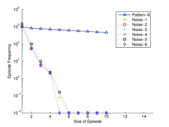
Figure 7: Statistical significance results for parallel episodes. Comparison of maximum frequencies of parallel episodes of different sizes for data with no structure and and minimum frequencies for data containing embedded patterns. Noise-1 to Noise-6 represent different types of data with no structure in it as explained in text. Pattern-8 refers to data generated with a model containing a synchrony pattern of size 10

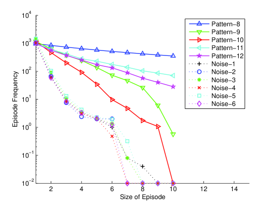
Figure 8: Statistical significance results for serial episodes. Comparison of maximum frequencies of serial episodes of different sizes for data with no structure and minimum frequencies for data containing embedded patterns. Noise-1 to Noise-6 represent different types of data with no structure in it as explained in text. Pattern-8 to Pattern-12 refer to to data generated with a model containing a ordered pattern of size 10. These different data sets differ in the strength of interconnection between successive neurons in the serial pattern embedded. Pattern-8, Pattern-9 and Pattern-10 contain connections which correspond to the conditional probability value for firing of the next neuron as 0.8, 0.6 and 0.4 respectively. All these are obtained using the sigmoidal function for updating rate of firing. Pattern-11 and Pattern-12 are with connection strengths that correspond to conditional probability values of 0.8 and 0.7 respectively and these are generated using the linear model for updating the rate of firing.

The results for parallel episodes are shown in fig. 7 and those for serial episodes are shown in fig. 8. Note that in both figures we have used a log scale on the Y-axis. The figures show how average frequency varies with size in each type of data sets. As explained above, for the case of noise data, namely Noise-1 to Noise-7, what is plotted is average of maximum observed episode frequency versus size of episode. For case of pattern data, what is plotted is the average of minimum frequency of episodes that are part of the embedded pattern.

From fig. 7, it is clear that frequencies of parallel episodes that are part of the embedded patterns are higher by two orders of magnitude compared to those in noise data even at size 3. Also, frequencies of parallel episodes in noise data rapidly fall to zero with size. However, up to the size of embedded pattern, frequencies of parallel episodes of all sizes that are part of the embedded pattern remain very high. This clearly demonstrates that you can not get such episodes of large size with appreciable frequency unless the underlying data generation model has biases for the required type of coordinated firing.

From fig. 8, similar trends are seen for serial episodes also. The frequencies in case of noise data fall to zero quickly with increasing size of episodes and are also orders of magnitude smaller than those for data with patterns. In addition, in this figure we can see a clear empirical demonstration of our intuitive idea of why data mining can uncover the strong connections. Here we have used five different types of data with serial patterns with different data having interconnections of different strengths. As explained earlier, the weight of interconnection can also be equivalently specified in terms of the conditional probability, $\rho$. We show here cases of pattern data where the conditional probabilities vary from 0.4 to 0.8. At high conditional probability, all episode frequencies remain high up to size 10. But as the conditional probability is decreased, the frequencies come down. For example, when the conditional probability is only 0.4, the frequencies of episodes come down appreciably with size of episodes (even though they are still higher than those for noise data sets). Looking at the curves corresponding to the five cases of data with patterns, we see that decrease of episode frequency with size is directly related to how strong are the connections among neurons in the embedded patterns. Thus, we can say that long episodes with high frequencies can not come about unless there are strong interconnections (represented by the episodes) in the underlying data generation model.

The results presented in this subsection clearly demonstrate that when we find episodes with high frequencies they are statistically significant. Since the difference between maximum frequencies in Noise data and minimum frequencies in data with patterns is very high, it is fairly easy to select a frequency threshold. If we choose the same frequency thresholds as in our earlier examples on synthetic data, from the above figures, we see that there would be no frequent episodes under any of the noisy data. Since the average frequency of episodes under our null hypothesis (i.e., noisy data) are obtained from 150 samples (six noise models, each with 25 repetitions), we can say that the empirical probability of getting a frequent episode under our null hypothesis is less than $\frac{1}{150}$. Thus, (under this empirical estimate of probabilities) we can claim that the discovered frequent episodes are significant with a p-value of better than 0.006.

5.3 Analysis of multi-neuron data obtained from MEA experiments

In this subsection we present some of the results we obtained with our algorithms on multi-neuronal data obtained through multi-electrode array experiments. The data is obtained from dissociated cultures of cortical neurons grown on multi-electrode arrays. This is an extremely rich set of data where 58 cultures of varying densities are followed for five weeks. Everyday, the spontaneous activity as well as stimulated activity of each culture is recorded for different time durations. (See [6] for the details of experiments, nature of data, trends observed etc.). Since data was recorded from each culture for many days, one can presumably infer development of connections also. Here we only present a few of the results we obtained from analyzing the spontaneous data from these cultures, to illustrate the utility of our temporal data mining techniques on MEA data.

This data is not spike sorted and detected spikes are only assigned to the electrode on which the signal is recorded. Hence, in our data mining algorithm, the event types would be electrode names and not neurons. All our episodes only indicate connectivity patterns involving electrodes. However, by taking each occurrence of a detected frequent episode and looking at the raw signal at those times, it is possible to infer whether or not same neuron is involved in the spikes on that electrode. For the purposes of illustration here, we only discuss episodes in terms of electrodes. We note that such information is also very useful for making reasonable hypotheses regarding underlying connectivity patterns.

In these dissociated cortical cultures, there is a lot of spontaneous activity including many cycles of network-wide bursts [6]. Thus, patterns of coordinated firing by groups of neurons due to synapses, would be rare in the sense that the spikes which form the coordinated activity constitute only a small fraction of the total number of spikes output by the system. Thus, simple cross correlation based methods are not very effective in unearthing coordinated firing patterns. Using our algorithm for serial episode discovery under inter-event constraints, we are able to obtain some frequent episodes which remain frequent for a large number of days with increasing trend in frequency.

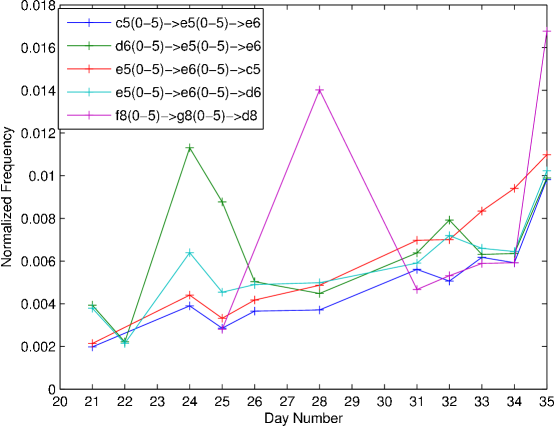
Figure 9: Some frequent Serial Episodes discovered from multi-electrode array data. We plot the normalized frequency versus the age in days of the culture. These are from data of culture 2-1 of Wagenaar, Pine, and Potter (2006)[6].

Fig. 9 shows a few such serial episodes discovered in the data from one of the cultures. (We have used inter-event time constraint of 1–5 ms). The figure plots the frequency (in terms of the number of non-overlapping occurrences as a fraction of the data length) for the frequent serial episodes versus the day on which the data is collected. In the figure, c5, e5, e6, d6 etc. are the pin numbers (or electrode names) in the multi-electrode array which will be event types for the data mining algorithms. The increasing trend of the frequency is very clear and it is highly plausible that these episodes represent some underlying microcircuits that are developing as the culture ages.

In this data, there is no ground truth available regarding connections and hence it is not possible to directly validate the discovered episodes. However, we can indirectly get some evidence that the episodes capture some underlying structure in the neural system by looking at the sets of episodes obtained from same culture on different days and from different cultures. We considered six cultures, namely, culture 2-1 to culture 2-6. For each culture we considered the data from the last five days, namely days 31 to 35. (As we have seen from the earlier figure, the circuits seem to stabilize only in the last week). However, in our data set, for culture 2-4 there was no recording on day 34 Thus we have 29 data sets such as 2-1-31 (meaning culture 2-1, day 31) and so on. From each culture on each day, we have 30 minutes of data recording spontaneous activity. From each data set, we have taken a 10 minute duration data slice. From each such data slice, we identified top twenty most frequent 7-node serial episodes with inter-event interval constraint of 1–5 ms. (We want to consider long episodes because, as we saw earlier, it is highly unlikely to have large size frequent episodes by chance. The size of 7 is chosen so that all data sets have at least twenty episodes of that size). Now we want to compare the sets of episodes discovered from different data slices. For this we need a measure of similarity between sets of episodes.

We define a similarity score for two sets, $A,B$, of episodes of size, say, N, as follows. We first count the number of N-node episodes that are common in the two sets and remove all the common ones from both sets. Then we replace each episode (in each set) with the two (N-1)-node subepisodes obtained by dropping the first or last nodes in the original episode. We now count the common (N-1)-node episodes (in the two sets) and remove them. We go on like this, by replacing the left-over episodes with subepisodes of size one less and counting the common ones, till we reach episodes of size 1. Let $n_{i}$ denote the number of common episodes of size $i$. Then the similarity between the sets $A$ and $B$ is defined as

$$\mbox{Sim}(A,B)=\sum_{i=1}^{N}\;2^{i}n_{i}.$$

Since we want to view episodes as representing connections, similarity has to capture how much of the paths represented by different episodes are common. The above measure does just that and gives higher weightage to common long episodes. We would like to point out that this particular similarity score is rather arbitrary and is used only for illustration.

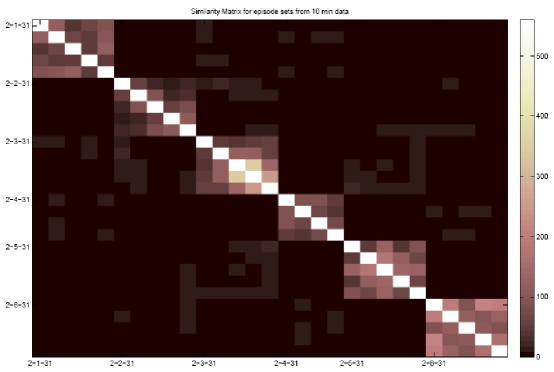
Figure 10: Cross similarity between sets of frequent Serial Episodes. Each pixel represents the similarity score between two sets of frequent episodes. Each axis consists of groups of (culture-dish) combinations going from 2-1 to 2-6. In each group, 5 days (i.e. day 31 to day 35) of recording are shown with label given to the start day (e.g. 2-1-31). The reverse diagonal corresponds to the case where the two sets of frequent episodes are identical. The similarity values are represented by different gray levels as explained by the legend on the right. Note the high similarity scores around the reverse diagonal. It shows that sets of episodes from the same culture have higher similarity than those from different cultures.

Fig. 10 shows the cross-similarity between the sets of frequent episodes from the 29 data slices by color coding similarity values. The axes indicate the culture-day combinations. Note that the two axes are ordered differently so that the reverse diagonal represents similarity between identical sets of episodes. That is why the reverse diagonal has highest similarity values. What is interesting is that data slices from the same culture but from different days are highly similar. This can be seen by observing the $5\times 5$ submatrices around the reverse diagonal in the figure. (For the 2-4 culture, this submatrix is only $4\times 4$ because there is no data for 2-4-34). This is in sharp contrast to the fact (as seen from the figure) that sets of episodes obtained from different cultures have very low similarity.

That the set of frequent episodes characterizes a culture like this, is interesting. In such cultures, qualitatively the spiking behavior observed in all cultures is very similar [6]. Since these cultures are seeded by the same cortical neurons and grow with time, they most likely form random interconnection patterns. Thus, the interconnectivity pattern may be the only thing that distinguishes one culture from another. Thus, our results seem to point out that the frequent episodes capture, in some sense, the underlying connectivity pattern. We feel that our results on synthetic data along with the results presented in this subsection provide sufficient justification that our temporal data mining techniques constitute a promising approach for analyzing multi-neuronal spike train data.

6 Discussion

Analyzing multi-neuron spike data is a challenging problem of much current interest in neuroscience. With the recent advances in experimental techniques, we can now easily obtain data representing the simultaneous activity of hundreds of neurons. Hence algorithms that can discover significant patterns of co-ordinated spiking activity among neurons would be very useful in making sense of these vast amounts of data. Discovering such patterns would help in understanding the underlying connectivity structure in the neural tissue and to relate it to the function of the nervous system. Such an understanding of the behavior of interacting neurons is very useful in elucidating issues such as learning and memory as well as for applications such as brain computer interfaces.

The main objective of this paper is to show the utility of a class of temporal data mining techniques for the above. We have introduced the notion of mining for frequent episodes with temporal constraints and have presented algorithms for finding such frequent episodes from large data streams. We have shown how one can detect many coordinated firing patterns in multi-neuronal spike data, such as order, synchrony, and synfire chains in terms of episodes with appropriate temporal constraints. We illustrated the effectiveness of the algorithms by analyzing synthetically generated spike sequences that have embedded patterns in them. For this we have modeled each neuron as an inhomogeneous Poisson process whose spiking rate gets modified in response to the input received from other neurons. By building an interconnected system of such neurons with some specific large excitatory connections along with many small random connections, we can embed different patterns in the system that is generating the spike data. Since the ground truth is known in these sequences, they serve as useful test beds for assessing the capabilities of our algorithms. We have shown that our algorithms unerringly discover the underlying connectivity structure. We have also shown that our algorithms can properly choose the inter-event temporal constraints by using data generated by networks where different synapses have different delays.

We have also used our neuronal spike data simulator to study the statistical significance of discovered frequent episodes. We have generated many sets of random data of both independent and dependent neurons but without any strong synapses. It is seen that the maximum frequency of episodes in such noise data are orders of magnitude smaller than minimum frequencies of relevant episodes when data contains patterns. Also the frequencies of episodes fall off very rapidly with the size (length) of the episodes in noise data when compared with that in data generated using some strong interconnections among neurons. These empirical results provide strong evidence that long episodes with appreciable frequencies can not come up by chance if the underlying system does not have the needed connectivity pattern. This, we feel, is a very significant contribution of this paper because the null hypothesis we consider here goes beyond the usual one of independent homogeneous Poisson processes. We have also provided some evidence for the effectiveness of these methods by analyzing data obtained from cortical neurons cultured on multi electrode arrays.

The data mining techniques discussed here are very efficient computationally. In addition to this, data mining techniques are attractive because such algorithms are model independent in the sense that they do not need to assume anything regarding a model for the interacting neurons. We have used two different methods of updating the firing rate of a neuron in response to inputs received from others. These result in different spike trains and the number of occurrences of different episodes are also different. However, the frequent episode discovery method is very good at inferring the underlying connectivity structure irrespective of the model followed for data generation.

The algorithms and results presented here should be viewed as indicative of the potential of temporal data mining for this problem. An objective of this paper is to introduce the problem multi-neuron spike data analysis to data mining community. Though this is a very challenging problem of analyzing large data sets to find underlying patterns, there does not seem to be much work in exploring data mining techniques for this problem. One can think of this problem as one of unearthing the network connectivity pattern given only node-level dynamic data. Such a problem would be relevant in many other application areas as well. For example, analyzing abnormal behavior of communication networks, finding hidden causative chains in complex manufacturing processes controlled by distributed controllers, etc. We hope our work presented here would contribute toward developing of data mining techniques relevant in such applications as well.

There are many open issues in the methods presented here. While the serial episodes with inter-event constraints give us a good idea of connectivity pattern, they do not allow us to infer the exact connectivity pattern or the graphical structure. For example, consider a circuit where $A$ is connected to $B$ with a synapse of delay 5 ms and $A$ is also connected to $C$ with a synapse of delay 10 ms. Hence, every time $A$ spikes, $B$ will spike 5ms later (with a large probability) and $C$ will spike another 5ms later. Thus serial episodes $A\rightarrow B$, $B\rightarrow C$, $A\rightarrow B\rightarrow C$ with inter-event time of 5ms and serial episode $A\rightarrow C$ with inter-event time of 10ms would all be frequent. Now suppose there is also a synapse between $B$ and $C$ of 5ms delay. Even then, the same set of episodes would be frequent. Thus the episodes alone can not completely determine the connectivity structure. In this example, the difference would be that, in one case every occurrence of the $B\rightarrow C$ episode would be part of an occurrence of $A\rightarrow B\rightarrow C$ episode while in the other case it is not. Thus, more algorithmic as well as statistical techniques are needed to infer the circuits completely given the episodes. Another direction in which the work of this paper can be extended is in developing a proper analytical hypothesis testing framework for assessing statistical significance of the episodes with a null hypothesis that allows for weak interactions among neurons. The techniques presented in this paper are useful in unearthing information regarding only those connectivity patterns which are due to excitatory synapses because the search is for frequently occurring episodes. The neural circuits contain both excitatory as well as inhibitory synapses. Developing data mining methods to infer inhibitory connections would be another major extension of this work. We would be addressing these issues in our future work.

Analyzing multi-neuronal spike data to finally obtain useful information about the underlying functional connectivity is a challenging problem. It would need an interdisciplinary approach and concerted effort by many researchers to solve this problem to any reasonable level. From signal-processing techniques for detection & temporal localization of spiking events to analytical techniques for properly understanding their statistics, many different methods and algorithms are needed here. The point we wish to make is that the field of data mining has an important role to play. We hope that our paper contributes toward development of novel data mining techniques useful in this endeavor.

Acknowledgments

We would like to thank Mr. Arvind Murthy for all the results presented in Sec. 5.3. This work is partially supported by project funding from General Motors R&D Center through SID, IISc.

Appendix A Pseudo-code listing for Algorithms in the paper

Algorithm 2 Non-overlapped count for parallel episodes with expiry time constraint

0:  Set $C$ of candidate $N$-node parallel episodes, event streams $s=\langle(E_{1},t_{1}),\ldots,(E_{n},t_{n})\rangle$, frequency threshold $\lambda_{min}\in[0,1]$, expiry time $T_{x}$

0:  The set $F$ of frequent serial episodes in $C$

1:  for all event types $A$ do

2:     $waits(A)=\phi$

3:  for all $\alpha\in C$ do

4:     Initialize $autos(\alpha)=\phi$

5:  for all $\alpha\in C$ do

6:     for all event types $A\in\alpha$ do

7:        Create node $s$ with $s.episode=\alpha$; $s.init=0$ ;

8:        $s.count=1$

9:        Add $s$ to $waits(A)$

10:        Add $s$ to $autos(\alpha)$

11:     Set $\alpha.freq=0$

12:     Set $\alpha.counter=0$

13:  for $i=1$ to $n$ do

14:     for all $s\in waits(E_{i})$ do

15:        Set $\alpha=s.episode$

16:        Set $j=s.count$

17:        if $j>0$ then

18:           Set $s.count=j-1$

19:           $\alpha.counter=\alpha.counter+1$

20:        $s.init=t_{i}$

21:        {Expiry check}

22:        if $\alpha.counter=N$ then

23:           for all $q\in autos(\alpha)$ do

24:              if $(t_{i}-q.init)>T_{x}$ then

25:                 $\alpha.counter=\alpha.counter-1$

26:                 $q.count=q.count+1$

27:        {Update episode count}

28:        if $\alpha.counter=N$ then

29:           Update $\alpha.freq=\alpha.freq+1$

30:           Reset $\alpha.counter=0$

31:           for all $q\in autos(\alpha)$ do

32:              Update $q.count=1$

33:  Output $F=\{\alpha\in C$ such that $\alpha.freq\geq n\lambda_{min}\}$

Algorithm 3 Non-overlapped serial episodes count with inter-event interval constraints

0:  Set $C$ of candidate $N$-node parallel episodes, event streams $s=\langle(E_{1},t_{1}),\ldots,(E_{n},t_{n})\rangle$, frequency threshold $\lambda_{min}\in[0,1]$, expiry time $T_{X}$

0:  The set $F$ of frequent serial episodes in $C$

1:  for all event types $A$ do

2:     Initialize $waits(A)=\phi$

3:  for all $\alpha\in C$ do

4:     Set $prev=\phi$

5:     for $i=1$ to $N$ do

6:        Create $node$ with $node.visited=false$; $node.episode=\alpha$; $node.index=i$; $node.prev=prev$; $node.next=\phi$

7:        if $i=1$ then

8:           Add $node$ to $waits(\alpha[1])$

9:        if $prev\neq\phi$ then

10:           $prev.next=node$

11:  for $i=1$ to $n$ do

12:     for all $node\in waits(E_{i})$ do

13:        Set $accepted=false$

14:        Set $\alpha=node.episode$

15:        Set $j=node.index$

16:        Set $tlist=node.tlist$

17:        if $j<N$ then

18:           for all $tval\in tlist$ do

19:              if $(t_{i}-tval.init)>\alpha.t_{high}[j]$ then

20:                 Remove $tval$ from $tlist$

21:        if $j=1$ then

22:           Update $accepted=true$

23:           Update $tval.init=t_{i}$

24:           Add $tval$ to $tlist$

25:           if $node.visited=false$ then

26:              Update $node.visited=true$

27:              Add $node.next$ to $waits(\alpha[j+1])$

28:        else

29:           for all $prev\_tval\in node.prev.tlist$ do

30:              if $t_{i}-prev\_tval\in(\alpha.t_{low}[j-1],\alpha.t_{high}[j-1]]$ then

31:                 Update $accepted=true$

32:                 Update $tval.init=t_{i}$

33:                 Add $tval$ to $tlist$

34:                 if $node.visited=false$ then

35:                    Update $node.visited=true$

36:                    if $node.index\leq N-1$ then

37:                       Add $node.next$ to $waits(\alpha[j+1])$

38:              else

39:                 if $t_{i}-prev\_tval>\alpha.t_{high}[j-1]$ then

40:                    Remove $prev\_tval$ from $node.prev.tlist$

41:        if $accepted=true$ and $node.index=N$ then

42:           Update $\alpha.freq=\alpha.freq+1$

43:           Set $temp=node$

44:           while $temp\neq\phi$ do

45:              Update $temp.visited=false$

46:              if $temp.index\neq 1$ then

47:                 Remove $temp$ from $waits(\alpha[temp.index])$

48:              Update $temp=temp.next$

49:  Output $F=\{\alpha\in C$ such that $\alpha.freq\geq n\lambda_{min}\}$

References

- [1] A. Amarasingham. Statistical methods for the assessment of temporal structure in the activity of the nervous system. PhD thesis, Division of Applied Mathematics, Brown University, Providence, RI, USA, 2004.
- [2] A. Date, E. Bienenstock, and S. Geman. On the temporal resolution of neural activity. Technical report, Division of Applied Mathematics, Brown University, Providence, RI, USA, 1998.
- [3] A. K. Lee and M. A. Wilson. A combinatorial method for analyzing sequential firing patterns involvingan arbitrary number of neurons based on relative time order. J Neurophysiol, 92(4):2555–2573, 2004.
- [4] A. K. Lee and M. A. Wilson. Memory of sequential experience in the hippocampus during slow wave sleep. Neuron, 36(6):1183–1194, Dec 2002.
- [5] A. Riehle, F. Grammont, M. Diesmann, and S. Grun. Dynamical changes and temporal precision of synchronized spiking activity in monkey motor cortex during movement preparation. Journal of Physiology-Paris, 94(5-6):569–582, 2000.
- [6] D. A. Wagenaar, J. Pine, and S. M. Potter. An extremely rich repertoire of bursting patterns during the development of cortical cultures. BMC Neurosci, 7:11–11, 2006.
- [7] D. H. Perkel, G. L. Gerstein, and G. P. Moore. Neuronal spike trains and stochastic point processes II: simultaneous spike trains. Biophysical Journal, 7:419–440, 1967.
- [8] D. R. Brillinger. Nerve cell spike train data analysis: a progression of thechniques. J. Am. Statist. Assoc., 87:260–271, 1992.
- [9] D. Patnaik. Application of frequent episode discovery framework in micro electrode array data analysis. Masters thesis, Indian Institute of Science, June 2006.
- [10] E. M. Izhikevich. Polychronization: computation with spikes. Neural Computation, 18(2):245–282, Feb 2006.
- [11] E. N. Brown, R. E. Kass, and P. P. Mitra. Multiple neural spike train data analysis: state-of-the-art and future challenges. Nat Neurosci, 7(5):456–461, May 2004.
- [12] F. Bonchi and C. Lucchese. Extending the state-of-the-art of constraint-based pattern discovery. Data and Knowledge Engineering, 60(2):377–399, 2007.
- [13] F. Morchen. Unsupervised pattern mining from symbolic temporal data. SIGKDD Explorations, 9:41–55, 2007.
- [14] F. Rigat, M. Gunst, and J. Pelt. Bayesian modelling and analysis of spatio-temporal neuronal networks. Bayesian Analysis, 1(4):733–764, 2006.
- [15] F. Zhang, L. P. Wang, M. Brauner, J. F. Liewald, K. Kay, N. Watzke, P. G. Wood, E. Bamberg, G. Nagel, A. Gottschalk, and K. Deisseroth. Multimodal fast optical interrogation of neural circuitry. Nature, 446(7136):633–639, Apr 2007.
- [16] G. L. Gerstein. Searching for significance in spatio-temporal firing patterns. Acta Neurobiol Exp (Wars), 64(2):203–207, 2004.
- [17] G. L. Gerstein, D. H. Perkel, and J. E. Dayhoff. Cooperative firing activity in simultaneously recorded populations of neurons: detection and measurement. J Neurosci, 5(4):881–889, Apr 1985.
- [18] G. L. Gerstein and D. H. Perkel. Simultaneously recorded trains of action potentials: analysis and functional interpretation. Science, 164(881):828–830, May 1969.
- [19] H. Mannila, H. Toivonen, and A. I. Verkamo. Discovery of frequent episodes in event sequences. Data Mining and Knowledge Discovery, 1(3):259–289, September 1997.
- [20] I. V. Tetko and A. E. Villa. A pattern grouping algorithm for analysis of spatiotemporal patterns in neuronal spike trains: I. detection of repeated patterns. J Neurosci Methods, 105(1):1–14, Jan 2001.
- [21] K. A. Ludwig, J. D. Uram, J. Yang, D. C. Martin, and D. R. Kipke. Chronic neural recordings using silicon micro electrode arrays electrochemically deposited with a poly(3,4-ethylenedioxythiophene) (pedot) film. J Neural Eng, 3(1):59–70, Mar 2006.
- [22] K. D. Wise, D. J. Anderson, J. F. Hetke, D. R. Kipke, and K. Najafi. Wireless implantable microsystems: high-density electronic interfaces to the nervous system. Proceedings of the IEEE, 92(1):76–97, Jan 2004.
- [23] K. P. Unnikrishnan, D. Patnaik, and P. S. Sastry. Discovering patterns in multi-neuronal spike trains using the frequent episode method. Technical report, 2007. available at http://www.citebase.org/abstract?id=oai:arXiv.org:0709.0566.
- [24] K. P. Unnikrishnan, N. Ramakrishnan, P. S. Sastry, and R. Uthurusamy. Network reconstruction from dynamic data. In ACM SIGKDD Explorations, 8(2) (2006),90-91.
- [25] K. P. Unnikrishnan and R. Uthurusamy. Proceedings of the KDD 2001 Workshop on Temporal Data Mining, Aug 2001; In http://www.sigkdd.org/kdd2001/Workshops/TemporalMiningWorkshop.html.
- [26] K. P. Unnikrishnan, R. Uthurusamy, and J. Han. The Third SIGKDD Workshop on Mining Temporal and Sequential Data (KDD/TDM 2004). In ACM SIGKDD Explorations, 6(2) (2004), 152.
- [27] M Abeles. Corticonics: Neural Circuits of the Cerebral Cortex. (New York: Cambridge University Press, 1991).
- [28] M. Abeles and I. Gat. Detecting precise firing sequences in experimental data. J Neurosci Methods, 107(1-2):141–154, May 2001.
- [29] M. Abeles and G. L. Gerstein. Detecting spatiotemporal firing patterns among simultaneously recorded single neurons. J Neurophysiol, 60(3):909–924, Sep 1988.
- [30] M. A. L. Nicolelis, D. Dimitrov, J. M. Carmena, R. Crist, G. Lehew, J. D. Kralik, and S. P. Wise. Chronic, multisite, multielectrode recordings in macaque monkeys. PNAS, 100(19):11041–11046, 2003.
- [31] M. J. Schnitzer and M. Meister. Multineuronal firing patterns in the signal from eye to brain. Neuron, 37(3):499–511, Feb 2003.
- [32] M. J. Zaki. Sequence mining in categorical domains: Incorporating constraints. In Proc. ACM 9th Int. Conf. Information and Knowledge Management (CIKM), Washington, DC, USA, November 2000.
- [33] M. Meister. Multineuronal codes in retinal signaling. Proc Natl Acad Sci U S A, 93(2):609–614, Jan 1996.
- [34] M. Meister, J. Pine, and D. A. Baylor. Multi-neuronal signals from the retina: acquisition and analysis. J Neurosci Methods, 51(1):95–106, Jan 1994.
- [35] M. O. Heuschkel, M. Fejtl, M. Raggenbass, D. Bertrand, and P. Renaud. A three-dimensional multi-electrode array for multi-site stimulation and recording in acute brain slices. J Neurosci Methods, 114(2):135–148, Mar 2002.
- [36] P. Dayan and L. F. Abbott. Theoretical Neuroscience: Computational and Mathematical Modeling of Neural Systems. Cambridge MA: MIT Press, 2005.
- [37] R. Agrawal and R. Srikant. Mining sequential patterns. In Philip S. Yu and Arbee S. P. Chen, editors, Eleventh International Conference on Data Engineering, pages 3–14, Taipei, Taiwan, 1995. IEEE Computer Society Press.
- [38] R. E. Kass, V. Ventura, and E. N. Brown. Statistical issues in the analysis of neuronal data. J Neurophysiol, 94(1):8–25, Jul 2005.
- [39] R. J. Vetter, J. C. Williams, J. F. Hetke, E. A. Nunamaker, and D. R. Kipke. Chronic neural recording using silicon-substrate micro electrode arrays implanted in cerebral cortex. IEEE Trans Biomed Eng, 51(6):896–904, Jun 2004.
- [40] S. Laxman, P. S. Sastry, and K. P. Unnikrishnan. A fast algorithm for finding frequent episodes in event streams. In Proc. ACM SIGKDD Int. Conf. Knowledge Discovery and Datamining, San Jose, USA, August 2007.
- [41] S. Laxman, P. S. Sastry, and K. P. Unnikrishnan. Discovering frequent generalized episodes when events persist for different durations. IEEE Transactions on Knowledge and Data Engineering, 19(9):1188–1201, 2007.
- [42] S. Laxman. Discovering Frequent Episodes: Fast algorithms, connection with HMMs and generalization. PhD thesis, Indian Institute of Science, March 2006.
- [43] S. Laxman, P. S. Sastry, and K. P. Unnikrishnan. Discovering frequent episodes and learning hidden markov models: A formal connection. IEEE Transactions on Knowledge and Data Engineering, 17(11):1505–1517, 2005.
- [44] S. Laxman and P. S. Sastry. A survey of temporal data mining. SADHANA, Academy Proceedings in Engineering Sciences, 31(2) (2006), 173-198.
- [45] S. Orlando, R. Perego, and C. Silvestri. A new algorithm for gap constrained sequence mining. In Proc. ACM Symposium on Applied Computing, Nicosia, Cyprus, March 2004.
- [46] T. Hosoya, S. A. Baccus, and M. Meister. Dynamic predictive coding by the retina. Nature, 436(7047):71–77, July 2005.
- [47] T. Sasaki, N. Matsuki and Y. Ikegaya. Metastability of active CA3 networks. The Journal of Neuroscience, 27(3):517–528, 2007.
- [48] W. Bialek, F. Rieke, R. R. de Ruyter van Steveninck, and D. Warland. Reading a neural code. Science, 252(5014):1854–1857, 1991.
- [49] X. Han and E. S. Boyden. Multiple-color optical activation, silencing, and desynchronization of neural activity, with single-spike temporal resolution. PLoS ONE, 2(3), 2007.
- [50] Y. Ikegaya, G. Aaron, R. Cossart, D. Aronov, I. Lampl, D. Ferster, and R. Yuste. Synfire chains and cortical songs: temporal modules of cortical activity. Science, 304(5670):559–564, Apr 2004.