Wetting Problem
For Multi-Component Fluid Mixtures
Abstract
In this paper we propose an extension of the Cahn method [1] to binary mixtures and study the problem of wetting near a two-phase critical point without any assumption on the form of intermolecular potentials. A comparison between Cahn’s method and later works by Sullivan [2,3], Evans et al [4,5] is made. By using an expression of the energy of interaction between solid surface and liquids proposed recently by Gouin [6], we obtain the equations of density profiles and the boundary conditions on a solid surface. In the case of a convex free-energy, a one-dimensional solution of a linear problem is proposed for the density profiles between a bulk and on a solid wall. A non-linear model of binary mixtures [7] extending Cahn’s results for simple fluids is also studied. For the case of a purely attractive wall we have established a criterion of a first order transition in terms of the structure of the level set of the homogeneous part of the free energy. Additively, explicit expressions of density profiles near the wall are proposed. They allow one to consider the adsorption of mixture components by a solid wall.
keywords:
Wetting problem; fluid mixturesPACS:
: 68.45.Gand
1 Introduction
In 1977, Cahn [1] gave simple illuminating arguments to describe the
interaction between solids and liquids. His model was based on a generalized
van der Waals theory of fluids treated as attracting hard spheres [7]. It
entailed assigning to the solid surface an energy that was a functional of
the liquid density ”at the surface”. Three hypotheses are implicit in Cahn’s
picture for simple fluids:
In order for the liquid density to be a smooth function of the
distance from the solid surface, that surface is assumed to be flat on the
scale of molecular sizes and the correlation length is assumed to be greater
than intermolecular distances (this is the case, for example, when the
temperature is not far from the critical temperature ).
The forces between solid and liquid are of short range and can
be described simply by adding a special energy at the solid surface.
The fluid is considered in the framework of a mean field
theory. This means, in particular that the free energy of the fluid is a
classical so-called ”square-gradient functional”.
After Cahn, the problem of adsorption and wetting was studied by a
statistical method by Sullivan [2,3], Evans et al [4,5],
respectively for gas and binary fluid mixtures. From the point of view of
Sullivan and Evans et al one may view Cahn’s approach as open to
criticism for several reasons:
Cahn’s treatment is based on phenomenological ”square-gradient”
version of van der Waals theory, which in contrast to the approach initiated
by van Kampen [8] does not attempt to relate directly the properties of the
non-uniform fluid to the interactions occurring on a molecular level.
The density adjacent to the wall vary strongly over the range of
intermolecular forces, consequently the gradient expansion approximation
used in deriving the square-gradient theory is no longer valid.
Cahn’s theory leaves unspecified a contribution due to the
fluid-solid interfacial free energy.
Evans et al [4,5] following Sullivan’s approach [2,3] for simple
fluids consider the special case of a contact between a two-component
mixture near ”the critical end point” and a wall. They used Sullivan’s grand
potential to describe the solid-fluid and fluid-fluid interactions and tried
to solve directly the problem of repartition of densities in a liquid (gas).
Evans et al obtain a coupled system of integral equations for
chemical potentials (cf. Eq. (6) in [4]). Then, to solve the system, it is
necessary to know the interaction potentials between components and between
solid wall and components: Evans et al assume an exponential
interaction both for component-component and solid-components (as in [2,3]).
Only such a hypothesis allows one to obtain two differential equations
instead of the two integral equations (Eq. (10) in [4]). This assumption
cannot be obviously valid for large classes of mixtures. Moreover, a special
hypothesis (mixing rule) concerning interactions between components is
assumed. Then, the mixing rule and exponential dependence allow one to
obtain both the linear relation between potentials and boundary conditions
and the problem is reduced to the problem of the contact of one-component
fluid with a wall.
The phenomenological ”square-gradient” model is proposed in case of an
infinite non-homogeneous fluid or a fluid mixture as a small-gradient
approximation by Widom [9] and Fleming et al [10]. The method is
extended in mean-field theory for semi-infinite media in contact with a
wall: as proved in [6], the fact that the densities are discontinuous at the
solid wall does not disqualify the procedure used by Widom and Fleming
et al and Cahn’s treatment is valid for fluids and fluid mixtures
near a critical point in contact with a wall.
In this paper, we use the expression of a surface energy. The surface is assumed to be solid and interactions between solid and fluids are sufficiently short-range. The contribution of fluids is represented by a surface free energy with a density of the form , where and are the limiting densities of the fluid components at the surface. The expression of the surface energy obtained in [6] is in the form:
This expression represents first terms of a more complex expansion. It is an extension with explicit calculations of the widely known expression due to Nakanishi and Fisher [11] and examined in a review paper by de Gennes [12]. All the coefficients can be calculated explicitly after the particular form of interaction potentials was chosen. For example, in the case of London forces, the values of coefficients related to the densities of the two fluids at the surface are [6]
where is the density of the solid, are the coefficients associated with intermolecular potentials of
interaction between the fluids and the solid wall, are intermolecular potentials of interaction between the
molecules of fluid and themselves or between the two fluids and are the minimal distances between the solid and molecules of
the two species of the mixture, where is the diameter of molecule of fluid and for the solid.
Expression (1) allows us to estimate the influence of a solid wall on each
component of a fluid mixture. Depending on the values of coefficients , one can estimate the magnitude of the attraction or repulsion
effects due to the wall.
As our approach is also based on a mean-field approximation, we assume that
variations of densities near the wall take into account several molecular
ranges. Hence, it is possible to present the total free energy of the system
”fluids - wall” as the sum of a bulk free energy and a surface energy which
is an additional contribution arising from the non-uniformity of the fluid
near the wall. By using an extended variational principle, we obtain two
boundary conditions at the wall and two partial differential equations for
the density profiles of the components between a solid wall and a bulk. The
complete set of boundary conditions and equations for densities allow us to
obtain the profiles of densities in the following physical situations. The
first is the study of the linear problem associated with the equilibrium of
a two-component one-phase mixture near a critical point with a solid wall.
The second is the study of the non-linear problem of the contact between a
two-component two-phase mixture near a critical point and a wall. We get a
condition of wetting and a first order wetting transition in terms of the
level set of the homogeneous part of the free energy.
To clarify the presentation some calculations are situated in Appendices. In Appendix 1, we present general calculations by using an extended variational principle applied to multi-component mixtures. In Appendix 2 we give an analytical representation of the profiles of densities connecting bulk and solid wall for a general form of the free energy of a two-component mixture near any critical point. These representations may be used to investigate the adsorption of fluid components of a mixture by a solid wall.
2 Equations of density profiles and boundary conditions: general results
The general form of the free energy per unit volume of the mixture is proposed in the form [7,10,13]
where notes the gradient operator in the physical space . The associated total free energy is
The wall boundary of is endowed with a surface energy per unit area. The surface is solid and sharp on an atomic scale and the interactions between surface and fluids are sufficiently short range; the general form of the surface free energy per unit area used is
Consequently, the free energy of is
Then, the grand potential of the system ”fluid mixture - wall” is
The condition of extremum of the energy based on hypotheses (3) and (4) yields (see for details Appendix 1):
- Equations of two profiles of component densities:
where is the vector whose components are the partial derivatives of with respect to the components of and is the divergence operator.
- Two boundary conditions at the solid wall:
where is the external unit normal vector to .
Equations of equilibrium (5) are the same as in [7] given for the one-dimensional case. Conditions (6) generalize those proposed in [1].
3 The dynamical system associated with one-dimensional density profiles
In the simplest case, the surface energy per unit area is given by (1) where the coefficients are expressed by means of a mean-field approximation through the potentials of the intermolecular interactions (see for example (2)) and the free energy per unit volume is of the form
where is the homogeneous free energy per unit volume and are constants such that the corresponding quadratic form is positive definite (we denote the free energy by corresponding in [7] to ).
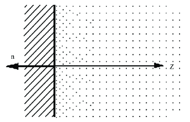
Let us consider the case of a flat plate wall defined by equation (see figure 1), where denotes the one-dimensional coordinate orthogonal to the wall. The equations of equilibrium (6) associated with (7) are
where and are two constants of integration.
These equations are complemented by the boundary conditions (6) at . By using expression (1) of the surface energy, we get
We have to add the condition in the bulk ():
4 Linear wetting problem
We consider the case of a one-phase mixture (liquid or gas) in contact with a solid wall. The densities of the two-components and the temperature are close to critical conditions. Moreover, we assume that density variations are small enough with respect to bulk densities, i.e.
such that we can consider a linearized problem associated with equations (8). Let us denote
The matrix is calculated in the bulk . Taking into account the definitions (11), we get the linearized problem associated with equations (8)-(10) in the form:
The stability of the thermodynamic state of the bulk requires that the symmetric matrix is also positive definite.
Let , be the eigenvalues and the eigenvectors of the equation
Since and are symmetric and positive definite, are positive. We can always suppose that111 denotes the bilinear form of vectors and with respect to matrix ; the bilinear form is symmetric when matrix is symmetric.
The solution of (12) satisfying the condition (14) is in the form
Substituting expression (15) into condition (13), we get a linear system of algebraic equations for the unknown coefficients
which defines a unique solution if . In particular, if is negligible (we assume that the wall is purely attractive), we get (see (11)) and
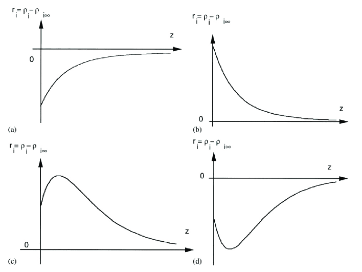
In such a case, the solutions satisfy conditions (13) and the density profiles fulfil the solution of linearized problem. Equations (15) yield different forms of density profiles. Depending on wall conditions, we may obtain both monotonic and non-monotonic profiles. This is similar to results of [7] in the non-linear case without a solid wall. In figure 2, we represent the different density profiles for each component of the mixture. We note that only one extremum point may appear for each density profile. This result is different from the results of Evans et al where density profiles are essentially monotonic.
5 Wetting problem near a critical point for a two-component mixture
5.1 The dynamical system
In a two-phase region near a critical point at a given temperature , the expression of the free energy per unit volume associated with a phase equilibrium is of the form [7]
The parameter is an independently varied field characterizing the ”distance” from the critical point , and are functions of the temperature. The variables and are defined through the transformation
The scalars associated with the physical properties of the mixture near the critical point depend on the temperature . The constants of integration and are already incorporated in . With Eq. (17), the system (8) can be rewritten in the form
where denotes the transpose matrix and means the gradient with respect to .
Following Rowlinson and Widom [7] we denote by
Obviously, if is positive definite, is also positive definite, i.e. , . The boundary conditions (9) at the wall are
In the following, we choose in Eq. (16) and (to do this, we have only to change the values of coefficients of the matrix defined by (17)). Hence, .
The system (18)-(19) yields
System (21) admits the first integral
This integral is similar to the integral of energy for mechanical problems.
Substitution of boundary conditions (20) into the relation (22) yields necessary conditions for at the solid wall. For simplicity, we consider only the case of an attractive wall ( is then negligeable). Conditions (20) yield
In fact, it is natural to expect that the results we obtain in the case of an attractive wall are closely similar to the results associated with the most general case. Relations (22) and (23) yield
where . Then, discussion of the wetting of a fluid mixture with a solid wall arises naturally from the drawing of the level curves of U(x,y) as a function of the parameter .
5.2 Connection between the dynamical system and Young’s conditions
For a solid wall in contact with phases and , the contact angle is defined with the help of surface free energies along the solid surface (Young’s conditions)
where the different subscripts designate phases adjoining the surface or interface. No value of satisfies Eq. (24) unless
If the inequality (25) is not satisfied, one of the fluid phases completely wets the solid and there is no contact between solid and other fluid phase. In fact, the forbidden surface is replaced by a layer of the wetting phase and the surface free energy becomes the sum of two surfaces’ free energies of the layer
Condition (26) corresponds to the perfect wetting with the solid. The surface energies can be calculated by the formulas
where and integrals are taken on different paths connecting phase and phase or a phase and the wall [7].
Let us note .
From the first integral (22), we get
The integrals (27) are calculated on the paths associated with system (21) and the boundary conditions on the wall
and in the bulks
5.3 Discussion of the wetting
For a solid wall the value of is given. Hence, the discussion depends on the relative value of parameter .
(a) and large enough.
In this case we are far enough from the critical conditions. In figure 3a the phases are in points and . One obtains easily that . The points and belong to two different connected components of the level set . In the vicinity of (or ), the energy is a convex function of and as in Section 4, it is possible to find the profiles of densities connecting and or and , respectively. The integrals (27) are positive and is large with respect to and . Then the relations
hold and we are in the case of partial wetting with .
(b) and small enough.
This case corresponds to phases close enough to the critical point (see figure 3b). The level set consists only of one connected component containing the points and . The phases are at the points and . They are very close with respect to the distance to the level curve. The superficial tension is small with respect to the free energies and . The values of and are in general different and one of the two relations (28) is not satisfied. We are in the case where one of the two phases wets completely the solid wall. No contact appears between the other phase and the solid. For exemple, if relation (26) is satisfied, the phase wets completely the wall.
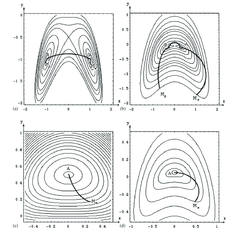
(c)
The mixture has only one phase at the point , which is the only singular point of the system (21). The energy attains a minimum at the point (we note that for this point corresponds to a saddle point, which is not associated with a bulk phase). The free energy of the mixture is convex at the vicinity of (figures 3c and 3d). If is small enough, the linear solution for the profiles of densities obtained in Section 4 can be used. When is large enough, the solution for the profiles of densities can be calculated analogously as in the Appendix 2.
5.4 Some remarks on the profiles of densities
The system (21) yields
and admits the first integral (22):
When the densities are far from critical conditions, is negligeable with respect to and and (30) reads
Let us denote Then, by using (29) and (31), we get . The right-hand side is a positive definite quadratic form, which implies that
Hence,
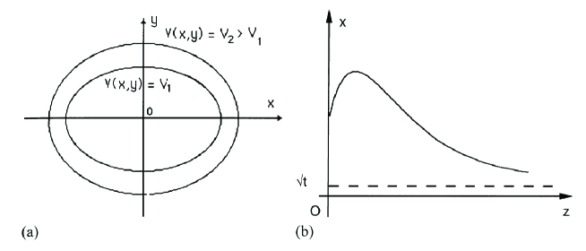
If , it follows from here that as . The level curves of are represented in figure 4a. Hence, or must be an increasing function of near the solid wall. For example, let be an increasing function of when is small enough. Due to the fact that as and is small with respect to the representation of as a function of has the form shown in figure 4b. Hence, the function is non-monotonic. In this case we may have also non-monotonic profiles of densities unlike in the treatment of Evans et al. Then, construction of an analytical solution may be done according to the algorithm proposed in Appendix 2.
6 Conclusion
Near critical conditions, by using a variational approach, we have obtained
for an isothermal binary mixture in contact with a solid wall equations of
equilibrium and boundary conditions which generalize those obtained by Cahn.
With limit conditions in the bulk, they form a closed boundary value
problem. When the free energy of the mixture is a quadratic form with
respect to the densities of components and their gradients, we get explicit
profiles of the densities in the one-dimensional case.
In the case of a purely attractive wall we have also established a criterion
of a first order transition, when a contact angle against a solid wall
becomes zero. This criterion is formulated in terms of the level set of the
function : , where depends on the boundary
conditions. If the level set is a connected set, two multi-component layers
exist: one layer with ordinary adsorption and the second one in contact with
the wetting layer. If the level set is disconnected we have partial wetting.
We have also shown that the profiles of density are typically non-monotonic.
This is in agreement with Rowlinson and Widom [7] where infinite two-phase
two-component mixtures where considered.
Acknowledgements
We have greatly benefited from comments and advises of Professor Benjamin Widom.
Appendix 1. Calculus of variations for fluid mixtures
We study a two-fluid equilibrium, but the method can be extended to any number of components. The position of a two-fluid mixture is associated with two applications
where denote the Lagrangian coordinates belonging to a reference space associated with the th component and denotes the Eulerian coordinates in the physical space [13]. The virtual motions of particles are deduced from the relation
Here are small parameters defined in a neighbourhood of zero. Virtual displacement are defined by [13,14]
At the solid boundary, the virtual displacement is subject to the conditions
where is the unit normal vector to the boundary.
Eulerian variations of densities are defined by
The variations (A3) are related to the virtual displacements (A1) by the formulae [14,15]
The variations of the volume free energy are
where
Since
we get
where the variational derivative is defined by
From relations (A2), (A4) and (A5) we obtain
The variations of the surface free energy are
The grand potential of the system is and its th variation is given by the formula
Denoting , we obtain
where denotes the surface divergence. Denoting by the tangential gradient to , we get finally
Consequently, the equations of equilibrium are
or
and the boundary conditions are
Due to the fact that is a direct consequence of relation on the surface, the only effective boundary conditions are , i.e.
Appendix 2. Analytical representation of the profiles of densities of a two-component mixture for the wetting problem near a critical point
Our purpose is to express analytically the profiles of densities of a two-phase mixture in contact with a solid wall. The free energy is given by (16) and the dynamical system for the profiles are given by
We notice that the matrix
is positive definite in the bulk phases where and . As in the Section 4, we can determine the positive eigenvalues defined from the equation
where all the matrix coefficients are calculated in the bulk. We obtain
For small enough, we get the two eigenvalues in the form
and
We are looking for the solution of the system (A8) which goes to the equilibrium states , at in the following form
We assume that this expansion is valid for all positive values of . We will show that this solution represents a two-parameter family. The values of the parameters will come from the boundary conditions (20). Substituting relations (A11) into (A8) and denoting and , we get
and
The identification of terms yields
The vectors and are eigenvectors corresponding to eigenvalues and defined by (A9) and (A10), respectively. The constants and are multipliers to be defined.
In the same way, the terms associated with and are
The expansion of truncated to the second order with respect to and is
Because the solution must be bounded as goes to zero for all positive values of , is at least of order . Then, we may introduce a constant by the formula
Since the terms and are of the order of , we get in the vicinity of
where all the coefficients are finite as goes to zero and . In fact, the term is negligible at the vicinity of the wall, but not in the bulk.
For the sake of simplicity, we exhibit the boundary conditions
only in the case of a purely attractive wall (when is negligible).
Then, the condition (20) on the wall reads
Or, by using (A13), we get
By multiplying (A14) by and , we get a system of two scalar equations. By taking into account the equality , the vector equation (A14) is equivalent to the system of two scalar equations
Eq (A15) defines and then, Eq. (A16) defines . Hence the solution near the wall (A13) is completely determined. Consequently, we are able to determine the effect of the solid wall on the adsorption of each component. Due to the fact that the expansion (A13) depends only on and not , in this approximation we do not need to satisfy the inequality .
References
[1] J. Cahn, J. Chem. Phys. 66 (1977) 3667.
[2] D.E. Sullivan, Phys. Rev. B 20 (1979) 3991.
[3] D.E. Sullivan, J. Chem. Phys. 74 (1981)
2604.
[4] M. Telo da Gama and R. Evans, Mol. Phys. 48
(1983) 687.
[5] I. Hadjiagapiou and R. Evans, Mol. Phys. 54
(1985) 283.
[6] H. Gouin, J. Phys. Chem. B 102 (1998) 1212.
[7] J.S. Rowlinson and B. Widom, Molecular Theory of
Capillarity, Clarendon Press, Oxford, 1984.
[8] N.G. van Kampen, Phys. Rev. B 135 (1964) A
362.
[9] B. Widom, J. Stat. Phys. 19 (1978) 563.
[10] P.D. Fleming, A.J.M. Yang, J.H. Gibbs, J. Chem. Phys.
65, (1976) 7.
[11] H. Nakanishi and M.E. Fisher Phys. Rev. Lett.
49 (1982) 1565.
[12] P.G. de Gennes, Rev. Mod. Phys. 57 (1985)
827.
[13] H. Gouin, Eur. J. Mech. B/ Fluids 9 (1990)
469.
[14] J. Serrin, Mathematical principles of classical fluid
mechanics, Encyclopedia of Physics, VIII/1, Springer, Berlin, 1959. pp.
125-263.
[15] S.L. Gavrilyuk, H. Gouin, Yu. V. Perepechko, C. R.
Acad. Sci. Paris II 324 (1997) 483.