Optimal control of atom transport for quantum gates in optical lattices

Abstract

By means of optimal control techniques we model and optimize the manipulation of the external quantum state (center-of-mass motion) of atoms trapped in adjustable optical potentials. We consider in detail the cases of both non interacting and interacting atoms moving between neighboring sites in a lattice of a double-well optical potentials. Such a lattice can perform interaction-mediated entanglement of atom pairs and can realize two-qubit quantum gates. The optimized control sequences for the optical potential allow transport faster and with significantly larger fidelity than is possible with processes based on adiabatic transport.

I Introduction

Quantum degenerate gases, such as Bose-Einstein condensates (BECs) bloch-review or cold Fermi gases inguscio-fermi , trapped in optical lattices, provide a flexible platform for investigating condensed matter models and quantum phase transitions bloch-qpt . It has been proposed to use these systems as quantum simulators of solid state systems cirac-chains and for implementing quantum information processing (QIP) brennen ; jaksch ; dorner . Experiments on neutral atoms have shown some of the ingredients needed for QIP: the preparation of a Mott insulator state with just one particle per well, which is used as the initial state of a quantum register bloch-qpt , single-qubit rotation lee07 , and controlled motion of atoms so as to effect entangling interactions mandelNature03 ; lee07 .

A general requirement of QIP is accurate control of a quantum system. Often this includes control of degrees of freedom other than the qubit or computational basis, for example the center of mass motion of an ion or atom for which the spin (internal state) represents the qubit. One approach to achieving such accurate control is adiabatic manipulation of the relevant Hamiltonian. Unfortunately adiabaticity limits the speed of operations. One way to overcome this difficulty is to use optimal control methods oc1 ; dorner . Here we show that such techniques could improve the speed and fidelity of transport of atoms in an optical lattice.

Recent experiments anderliniSwap ; mandelNature03 ; trotzky08a have shown that quantum gates could be implemented in controllable optical potentials by adjusting the overlap between atoms trapped in neighboring sites of an optical lattice. High fidelity of this dynamic process could be achieved by adiabatically changing the trapping potential. This, however, limits the overall gate speed to be much lower than the trapping frequency dorner ; garcia-2003 . Here we present a detailed numerical analysis of the transport process used to effect a two-qubit quantum gate in anderliniSwap , which is performed with the controllable double-well optical potential described in anderlini-pra and find that it gives an accurate description of the evolution measured in the experiment. Then we apply optimal control theory to the transport process of the atoms, both with and without interactions, to show how to increase the speed of the gate. The success of this method in this specific problem demonstrates the promise of optimal control for coherent manipulation of a diverse class of quantum systems.

II The experiment

A two-qubit quantum gate with neutral atoms can be realized in optical lattices through a controlled interaction-induced evolution of the wavefunction that depends on the states of the two atoms brennen ; jaksch . Because atoms in their electronic ground states generally have short-range interactions, in order to use these contact interactions to produce entanglement, the atomic wavefunctions must be made to overlap. Once the interaction has taken place for a fixed time, the two atoms can be separated again thus finishing the gate. In this paper we consider the control of such motion in a specific setup; however our theory can be applied to more general systems.

II.1 The Double-Well Lattice

Neutral ⁸⁷Rb atoms are loaded into the sites of a 3D optical lattice obtained by superimposing a 2D optical lattice of double-wells anderlini-pra in the horizontal plane and an independent 1D optical lattice in the vertical direction. The horizontal lattice has a unit cell that can be dynamically transformed between single-well and double-well configurations. The horizontal potential experienced by the atoms is anderliniJPhysB :

$$V(x,y) = -V_{0}\left[\cos^{2}\left(\frac{\beta}{2}\right)(\cos^{2}ky+\cos^{2}kx)+\right.$$ (1)

$$+ \left.\sin^{2}\left(\frac{\beta}{2}\right)(\cos ky+\cos(kx-\theta))^{2}\right]$$

where $x$ and $y$ are the spatial coordinates, $k=2\pi/\lambda$ is the laser wave-vector and $\lambda$ is the laser wavelength. The potential (1) depends on three parameters:

1. the strength $V_{0}$ of the potential wells;

2. the ratio $\tan\left(\frac{\beta}{2}\right)$ of vertical to horizontal electric field components;

3. the phase shift $\theta$ between vertical and horizontal light components.

The angle $\beta$ determines the height of the barrier between adjacent double-well sites: by changing $\beta/\pi$ from 0 to $0.5$ the potential changes from a symmetric double-well configuration, with a spacing of lambda/2 (lambda/2 lattice), to a single-well configuration, with a spacing of lambda (lambda lattice). By changing $\beta$ and $\theta$ together one varies the energy offset (tilt) of a well with respect to the neighboring one. The tilt of the double well is zero for $\theta/\pi$ = $\pm 0.5$, while it is maximum (with a value depending on $\beta$) for $\theta/\pi$ = 0 or $\pm\,1$.

To effect a quantum gate, one varies the three parameters in time so as to move atoms occupying adjacent wells into the same well, allowing them to interact and finally returning them to their original positions.

In Fig. 1 we show four snapshots of the cross-section of the optical potential along the direction of the double wells ($x$), and of the single-particle wave functions of the two atoms during a particular transport sequence. In the initial configuration each atom is prepared in the ground state of separate wells so that the properly symmetrized initial state is:

$$\left|\Psi_{\rm in}\right\rangle=\frac{1}{\sqrt{2}}\left(\left|\psi_{L}\right\rangle_{1}\left|\psi_{R}\right\rangle_{2}+\left|\psi_{R}\right\rangle_{1}\left|\psi_{L}\right\rangle_{2}\right)$$ (2)

where $\psi_{L}$ and $\psi_{R}$ are wavefunctions localized in the left and right well, respectively, and 1 and 2 are the labels of the two (indistinguishable) atoms (see Fig. 1a). For quantum gate operation, we would also include the internal state of the atoms, but here we concentrate only on the external state (center-of-mass motion). $\psi_{L}$ and $\psi_{R}$ are linear combinations of the lowest symmetric and antisymmetric energy eigenfunctions of the single-particle potential. In Eq. (2) and throughout the text we use the convention that single- (two-) particle states are labeled with lower (upper) case greek letters.

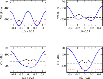
Figure 1: (Color online) a) Initial configuration: the potential (solid lines) is in the $\lambda/2$ configuration and the single-particle wave functions are localized in the left (dashed) or right (dotted) well. b)–c) Intermediate snapshots obtained by lowering the central barrier and tilting the potential. d) End of the process: the particle initially in the right well ends in the ground state of the single well, while the particle initially in the left well ends in the first excited state.

The potential is changed by lowering the barrier and at the same time lowering the right well with respect to the left one, Fig. 1b)-c). The atom initially in the right well remains in the ground state, evolving into the lowest state $\phi_{0}$ of the final potential, while the atom initially in the left well evolves into the first excited state $\phi_{1}$, Fig. 1d). When the two atoms are in the same potential well they interact through the usual contact interaction, which can be used to generate the entangling operation needed to realize a two-qubit quantum gate jaksch ; dorner .

II.2 Experimental Procedure

The experimental characterization of the transport process is accomplished by performing the potential transformation depicted in Fig. 1 with atomic samples loaded either only in the left sites or only in the right sites of the double wells anderliniJPhysB .

Briefly, Bose-Einstein condensates of ${}^{87}\textrm{Rb}$ atoms with $4\cdot 10^{3}\leq N_{\textrm{BEC}}\leq 2\cdot 10^{4}$ are loaded in the sites of the $\lambda$-lattice with an exponential ramp of 200 ms duration. This loading populates only the ground band of the optical potential with mostly one atom per lattice site SebbyPRL07 . Then the potential is transformed to the $\lambda/2$-lattice in such a way that the atoms eventually occupy either only the right sites or only the left sites of the double wells anderliniJPhysB ; lee07 . Starting from this initialized state, we perform the transport process illustrated in Fig. 1a)–d). At the end of the process we measure the occupation of the lattice bands. To this purpose, we map the quasi-momentum of atoms occupying different vibrational levels of the optical potential onto real momenta lying within different Brillouin zones kastberg95 ; greiner2001 . This is achieved by switching off the optical potential in 500 $\mu$s and acquiring an absorption image of the sample after a 13 ms time-of-flight. In this way atoms occupying different vibrational levels appear spatially separated, allowing us to measure the amount of population in each vibrational state.

The comparison between these measurements and the theoretical model requires an accurate determination of the evolution of the parameters $V_{0}$, $\beta$ and $\theta$ characterizing the optical lattice during the experimental sequences. The parameter $V_{0}$, which corresponds to the depth of the potential when it is set in the $\lambda/2$ configuration, is measured by pulsing the $\lambda/2$-lattice and observing the resulting momentum distribution in time of flight Ovchinnikov1998 . The parameters $\beta$ and $\theta$, which determine the shape of the double-well potential and are controlled using two electro-optic modulators (EOMs), are determined from measurements of the polarization of the laser beams after the EOMs as a function of their respective control voltages anderlini-pra .

We perform two series of experimental sequences in order to study the properties of the atomic transport as a function of the duration of the process and of the energy tilt between the two potential wells during the merge. In a first series of measurements the sequence involves converting the lattice from the double-well to the single-well configuration by changing $\beta$, rotating the polarization of the input light using a linear ramp, while leaving constant the light intensity and the setting of the electro-optic modulator EOM$\theta$ dedicated to the control of the phase shift $\theta$. This sequence is repeated for different durations of the linear ramp from $T=0.01$ ms to 1.01 ms. In a second series of measurements we consider the dependence of the transport on the tilt of the double-well potential during the merge. We perform the lattice transformation using always the same duration of $T=0.5$ ms, the same intensity of the light beam and the same ramp for changing the polarization angle $\beta$, while the the setting of EOM$\theta$ is kept constant in time during a sequence. We then repeat the sequence for different settings of EOM$\theta$. The time dependence for the three lattice parameters $V_{0}$, $\beta$ and $\theta$ for measurements of the first series and of the second series are shown in Fig. 2a and Fig. 2b, respectively. Fig. 2b shows the evolution of the parameter $\theta$ for two different settings of EOM$\theta$. The potential parameters are determined using our calibration of the lattice setup, taking into account effects such as different losses on the optical elements for different polarizations of the lattice beams and the dependence of the optical potential on the local polarization of the light lee07 . These effects are responsible for the change of the potential depth $V_{0}$ and of the angle $\theta$ during the sequence despite the fact that both the intensity of the light and the settings of EOM$\theta$ are not actively changed.

Figure 2: Two possible sequences a (left) and b (right) employed to shift the atoms from a double- to a single-well configuration are shown in the left and right part of the panel. For each sequence we show the time-dependence of $V_{0}$, $\beta$, $\theta$ for a sequence duration $T$. For sequence b we show the time dependence of $\theta$ for two settings of EOM$\theta$: $-0.42\;\pi$ (solid) and $-0.48\;\pi$ (dashed).

III Theoretical model

Here we describe the theoretical methods that we implement for investigating the dynamics in the system described above, starting with the case of non-interacting particles. Then, we consider the experimental realization of the merging of adjacent lattice sites into a single site shown in Fig. 1 and we compare the results obtained in the experiment with the expectations based on our theoretical model. This stage represents a useful benchmark to evaluate the reliability of the numerical model as well as for gaining insight into the details of the optical potential experienced by the atoms. Finally, we present the technique for optimizing the transport sequence, and we show how we can achieve a significantly higher fidelity at fixed operation time for the atomic motion than by using smooth sequences based on adiabatic evolution.

III.1 Theoretical Framework

We consider the 1D problem restricted to the x axis by assuming that the optical potential can be separated along the three spatial directions, allowing us to express the atomic wavefunctions as a product of three independent terms. We consider the harmonic approximation of the potential in the $y$ and $z$ directions, having trap frequencies $\nu_{y}$ and $\nu_{z}$ respectively, that can be calculated as shown in spielman06 and we assume that along $y$ and $z$ the atoms always occupy the lowest vibrational state. This restriction does not put limitations in studying dynamic processes involving low energy states of the double-well potential since it can be chosen to have non-degenerate vibration frequencies along all three directions, with the lowest frequency always along $x$. We calculate the eigenstates of the system along the $x$ direction by solving the eigenvalue equation using the finite difference method thomas . For the time evolution we consider the integration of the time dependent Schrödinger equation using the Crank-Nicolson method cn . This method has the advantage of being unconditionally stable and the error in the results scale quadratically with the number of space-time grid points in which the Schrödinger equation is solved. The relative error of the data presented is always less than $10^{-3}$. In Appendix A we present a more detailed description of our numerical methods.

III.2 Comparison to experimental results

In this section we present the theoretical analysis of the transport processes described above and we discuss the agreement between the model and the experimental measurements. We start by considering the time evolution of the Hamiltonian spectrum during the two sequences a and b shown in Fig. 3.

Figure 3: Instantaneous spectrum of the 1D Hamiltonian for sequences a and b for EOM$\theta$: $-0.42\;\pi$.

At time $t=0$ the spectrum is made of nearly degenerate doublets of almost equally spaced pairs of harmonic oscillator states, while at time $t=T$ the levels are similar to those of a single harmonic oscillator.

Fig. 3 shows the time evolution of the eigenstates of the single-particle Hamiltonian. The atoms initially prepared in the two local ground states in the right and left wells ($\psi_{R}$ and $\psi_{L}$) evolve into the instantaneous eigenstates ending in the ground and first excited state of the final configuration, respectively. This approach requires the sequence to be performed slowly with respect to the timescale associated with the gaps between the relevant energy levels. The optimal “speed” in the parameter space can be calculated using the Landau-Zener theory for avoided level crossings.

For gaining quantitative insight into the properties of the transport we perform numerical simulations for the sequences used in the experiments, also taking into account possible deviations of the parameters from the experimental calibrations, and we compare the results with the experimental measurements. The relevant quantities for our analysis will be the overlap $f^{\alpha}_{n}$ of the energy eigenstates $\phi_{n}$ of the final potential with the evolved state $\psi_{\alpha}$ where $\alpha=L,R$ indicates the initial well occupation:

$$f_{n}^{\alpha}=\left|\left\langle\phi_{n}\right|U(T)\left|\psi_{\alpha}\right\rangle\right|^{2}$$ (3)

where the operator $U(T)$ is the single-particle time-evolution operator from time $t=0$ to time $t=T$. In the experiment $f^{\alpha}_{n}$ can be measured as the population of each energy level at the end of the process.

We now consider how the atoms evolve when the parameters change according to sequence a of Fig. 2 as a function of the total time $T$, focusing on atoms starting in $\left|\psi_{L}\right\rangle$.

                                                

                                                

Figure 4: Population of the first three eigenstates of the Hamiltonian, ground (top), first excited (middle), second excited (bottom), at the end of sequence a as a function of the sequence duration $T$. The experimental data (symbols) are compared to the four sets of numerical data (lines) obtained for $\theta/\pi=-0.454+\Delta\theta_{a}/\pi$, with $\Delta\theta_{a}/\pi$ = 0 (dot-dash), -0.02 (dash), -0.03 (solid) and -0.04 (dot), while -0.454 is the nominal value of $\theta/\pi$ expected from the calibrations.

In Fig. 4 we show the final population of the ground $f_{0}^{L}$, first $f_{1}^{L}$ and second excited state $f_{2}^{L}$ measured in the experiments and calculated for four values of $\theta$ which differ from the one of Fig. 2 a by a constant offset $\Delta\theta_{a}$ . The results obtained by the model are in reasonable agreement with the experimental observations; we find best quantitative matching for $\Delta\theta_{a}/\pi$ = -0.03, for which the rms deviation between model and theory is reduced from 0.13(at $\Delta\theta=0$) to 0.08.

Now we consider the sequence b of Fig. 2, performed for different ending values $\theta_{b}$ of the parameter $\theta$ around $-0.47\pi$. As shown in Fig. 5, both the experiment and the model show a strong dependence on $\theta_{b}$ for the transport of the atom starting in the left site of the double well. The transport into the first excited state has a maximum theoretical fidelity of 0.95 for $\theta_{b}/\pi$ = -0.474. Less negative values of $\theta_{b}$, i.e. increasing tilts, lead to a decrease of fidelity due to the increase in the fraction of population ending in the second excited state. Values of $\theta_{b}/\pi$ closer to -0.5, i.e. more symmetric configurations of the double well, lead to decrease of fidelity associated with larger fractions of population ending in the ground state. Also in this case the experimental data and the theoretical model are in satisfactory agreement. For these data the deviation between theory and experiment is more sensitive to the value of the phase shift $\theta_{b}$. We find best agreement by shifting the value determined from the calibration by an offset $\Delta\theta_{b}/\pi$ = -0.015, which reduces the rms deviation from 0.4 to 0.15. The axis for the experimental data in Fig. 5 has been corrected by the offset $\Delta\theta_{b}$.

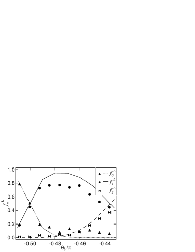
Figure 5: Population (overlap absolute squared) of the first three eigenstates of the Hamiltonian at the end of sequence b as a function of $\theta_{b}$. The duration of the sequence is fixed to $T=0.5$ ms. The experimental data (symbols) are in good agreement with the numerical data (lines). In this graph the $x$ axis for the experimental has been shifted by an offset of -0.015 with respect to the initial calibration.

Thus, while showing the reliability of the model in describing the dynamic process, the comparison between theoretical and experimental results also allows one to refine the calibration of the parameters characterizing the optical potential.

Finally we find that adding an offset of $\Delta\theta/\pi$ = -0.016 to the $\theta$ calibration brings the data from both sequences to a good agreement with the theory and reduces the rms deviation from 0.19 to 0.11. This is three times larger than the uncertainty of the offset from our EOM calibration but is still consistent with measurements of the lattice tilt from SebbyPRL07 . This discrepancy might be explained by the birefringence in the vacuum cell windows, which is not accounted for in our model. Inclusion of this offset should improve both the predictivity of the model and the experimental optimization of the collisional gate based on the numerical technique described below.

IV Optimized transport

In this section we employ optimal control theory to obtain fast and high-fidelity gates. Our aim is to find a temporal dependence of the control parameters $V_{0}(t)$, $\beta(t)$, $\theta(t)$ that improves the fidelity even for a shorter sequence duration, when the adiabatic sequences presented above yield a poor fidelity. Quantum optimal control techniques have been successfully employed in a variety of fields: molecular dynamics oc1 ; oc2 ; oc3 , dynamics of ultracold atoms in optical lattices tannor-2002 ; vaucher ; romero , implementation of quantum gates dorner ; monta-oc .

We use the Krotov algorithm krotov as the optimization procedure. The objective is to find the optimal shapes of the control parameter sequences that maximize the overlap (fidelity) between the evolved initial wave function and a target wave function. The initial and target wave functions are fixed a priori. The algorithm works also for more than one particle. The method consists in iteratively modifying the shape of the control parameters according to a “steepest descent method” in the space of functions (for more details see dorner ). The method requires evolving each particle’s wave function and an auxiliary wave function backward and forward in time according to the Schrödinger equations. In our simulations we use the Crank-Nicolson scheme to realize this step as described in Appendix A.

IV.1 Non-interacting case

We optimize the gate for $T=0.15$ ms choosing as a starting point for the optimization a sequence similar to Fig. 2b where $\theta$ is for simplicity taken constant to the final value $\theta_{b}/\pi=-0.474$. Without optimization the fidelities for the atom initially in the left and right well are $f^{L}_{1}=0.57$ and $f_{0}^{R}=0.69$, respectively. The infidelities are shown in Fig. 6 as a function of the number of optimization steps: the algorithm of optimization is proven to yield a monotonic increase in fidelity oc1 , however it does not guarantee to reach its 100% value. The results for the two atoms give a fidelity above $98.7\%$.

Figure 6: Infidelities ($1-f^{\alpha}_{n}$) for the atom initially in the left ($\alpha=L,n=1$, squares) and in the right well ($\alpha=R,n=0$, plus) as a function of the optimization step.

The resulting optimized parameter sequences are shown in Fig. 7 and compared to the original sequence without optimization. We find that the optimized sequence for the potential depth $V_{0}$ differs negligibly from the initial guess. In principle, the algorithm could achieve still higher single-particle fidelities from different starting points.

Figure 7: Initial (dotted) and optimized waveforms (solid) $\beta(t)$ and $\theta(t)$ as a function of time for a sequence of $T=0.15$ ms.

In Fig. 8 we show the square absolute value of the wave functions of the two atoms as a function of time, the 1D potential time dependence and the projections of the initially left-well state onto the lowest four instantaneous energy eigenstates $\left|\phi_{n}(t)\right\rangle$:

$$p_{n}(t)=\left|\left\langle\phi_{n}(t)\right|U(t)\left|\psi_{L}\right\rangle\right|^{2}.$$ (4)

Notice that $p_{n}(T)=f_{n}^{L}$. As can be easily seen, the optimal time evolution is much less smooth than the adiabatic one as it takes advantage of quantum interference between non-adiabatic excitation paths to obtain better results.

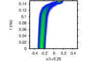
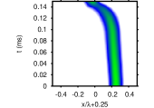
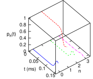
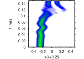
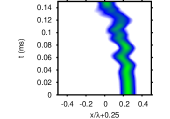
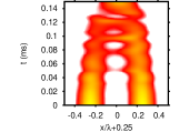
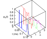
Figure 8: (Color online) Comparison between the evolution of the atoms with and without optimal control. Top (left to right): non optimized case, absolute square value of the wave functions as a function of time (atoms initially in the left and right well respectively); 1D trapping potential as a function of time; projections $p_{n}(t)$ at time $t$ of the state initially in the left well onto the instantaneous eigenstates $\left|\phi_{n}(t)\right\rangle$ with $n=0$ (blue solid), $n=1$ (red dashed), $n=2$ (green dotted), $n=3$ (magenta dot-dashed). Bottom: analogous plots for the optimized case.

IV.2 Interaction effects

Up to now we have considered only the single-particle evolution of the system, i.e. without including any interaction between the particles. This approximation is valid in our transport sequence as long as the two wave functions in nearby wells do not overlap. When the two particles overlap in the same well we must take into account interactions, and we model them with an effective 1D contact potential:

$$V_{\rm{int}}(|x_{1}-x_{2}|)=g_{1D}\delta(x_{1}-x_{2})$$ (5)

where $x_{i}$ are the coordinates of the two atoms and $g_{1D}$ is an effective $1D$ coupling strength olshanii expressed by $g_{1D}=2a_{s}h\sqrt{\nu_{y}\nu_{z}}$, where $a_{s}$ is the scattering length for ${}^{87}\mathrm{Rb}$ atoms and $h$ is the Planck constant. The spectrum is modified by the interactions: the state with one atom in each well is lower by $\sim 3$ kHz than the doubly-occupied states.

As in the case without interactions we start with each atom localized in a separate well. Notice that we are considering wave-functions that are symmetric under the exchange of the coordinates of the two particles.

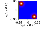
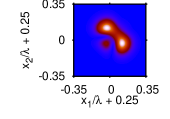
a b
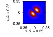
c d

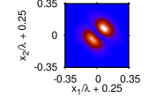
Figure 9: (Color online) Absolute square values of the relevant symmetric wave-functions in the coordinates of the two atoms: a Initial wave function in the state $\left|\tilde{\Psi}_{\rm in}\right\rangle$ with one atom in the left well and one atom in the right well; b wave function of the target state $\left|\tilde{\Phi}_{\rm tg}\right\rangle$. c evolved wave-function using the non-optimized sequences of Fig. 2b giving a fidelity $F_{\rm int}=0.22$ (for $T=150\mu$s); d evolved wave-function using the optimized sequences of Fig. 7 giving a fidelity $F_{\rm int}=0.93$.

We consider the two-particle fidelity:

$$F_{\rm int}=\left|\left\langle\tilde{\Phi}_{\mathrm{tg}}\right|U_{\textrm{int}}(T)\left|\tilde{\Psi}_{\mathrm{in}}\right\rangle\right|^{2}$$ (6)

where $U_{\textrm{int}}(T)$ is the two-particle evolution operator for the Hamiltonian of the two atoms, which includes interactions. $\left|\tilde{\Psi}_{\mathrm{in}}\right\rangle$ is an eigenstate of the two-particle Hamiltonian at time $t=0$, corresponding in the limit $g_{1D}\to 0$ to the symmetrized product of the single-particle wavefunctions localized in each well (see Eq.(2)); the target state $\left|\tilde{\Phi}_{\mathrm{tg}}\right\rangle$ is an eigenstate of the two-particle Hamiltonian at time $t=T$ which, in the limit of vanishing interactions, corresponds to the state

$$\left|\Phi_{\mathrm{tg}}\right\rangle=\frac{1}{\sqrt{2}}\left(\left|\phi_{0}\right\rangle_{1}\left|\phi_{1}\right\rangle_{2}+\left|\phi_{1}\right\rangle_{1}\left|\phi_{0}\right\rangle_{2}\right)$$ (7)

The square modulus of $\left|\tilde{\Psi}_{\mathrm{in}}\right\rangle$ and $\left|\tilde{\Phi}_{\mathrm{tg}}\right\rangle$, in the two-atom coordinate representation, are shown in Fig. 9a-b. In order to make a comparison between the interacting and non interacting cases we define a two-particle fidelity also in the non-interacting case:

$$F=\left|\left\langle\Phi_{\mathrm{tg}}\right|U_{1}(T)\otimes U_{2}(T)\left|\Psi_{\mathrm{in}}\right\rangle\right|^{2}$$ (8)

where $U_{1}(T)$ and $U_{2}(T)$ are the single-particle evolution operators for the two atoms without interactions.

	$f_{0}^{R}$	$f_{1}^{L}$	$F$	$F_{\rm int}$
non optimized	0.69	0.57	0.22	0.22
transport optimized	0.99	0.99	0.98	0.93
interaction optimized	0.98	0.98	0.96	0.97

Table 1: Results of our numerical simulations for three different sets of control parameters: the non optimized case Fig. 2b; the transport optimized case Fig. 7 where the optimal control algorithm is used without taking into account interactions; the interaction optimized case where the optimal control algorithm is used taking into account interactions. The quantities shown are: the single-particle populations $f_{0}^{R}$ and $f_{1}^{L}$ calculated without interactions, the two-particle fidelities $F$ and $F_{\rm int}$ calculated without and with interactions.

In Table 1 we summarize our results for $T=0.15$ ms obtained with three different sequences: first, the non optimized sequence Fig. 2b; second, the transport optimized case Fig. 7 where we used the optimal control algorithm to optimize the single-particle populations not taking into account interactions; third, the interaction optimized case where we apply the optimal control algorithm using as the initial guess the transport optimized sequence Fig. 7 and then optimizing including the interactions in the evolution.

The resulting wave-functions for the non optimized and transport optimized sequences are compared in Fig. 9c-d. Without optimal control the two-particle fidelity with and without interactions is $F=F_{\rm int}=0.22$ while with (non-interacting) optimization we obtain $F\simeq f_{0}^{R}\,f_{1}^{L}=0.98$ and $F_{\rm int}=0.93$. This shows that interactions spoil slightly the efficiency of the transport process as one might expect. Optimal control can subsequently be applied while including interactions in the optimization, producing a control sequence with a fidelity of $F_{\rm int}=0.97$.

Another consideration is the experimental bandwidth available for feedback control. The optimized control waveforms Fig. 7 were obtained with no restriction on the frequency response of the control, and typically have frequency components on the order of a few times the lattice vibrational spacings (see Fig. 10), i.e. larger than the bandwidth of our control electronics. Clearly, using a filtered version of these waveforms will lead to lower control fidelity and it will be important to increase the experimental bandwidth of the control electronics (currently about 50 kHz). In addition, it may be useful to develop an optimization sequence that includes the limited control bandwidth, although it is likely that frequencies on the order of the vibrational spacing will always be needed.

Figure 10: The normalized Fourier transform magnitudes $|\tilde{\beta}(f)|$ (solid) and $|\tilde{\theta}(f)|$ (dashed) of the optimized control sequences $\beta(t)$ and $\theta(t)$ shown in Fig. 7. The spectra are normalized to the value at the fundamental frequency $1/T=6.67$ kHz.

V Conclusions

We have presented a detailed, numerical analysis of the transport process of neutral atoms in a time dependent optical lattice. We show how to improve the fidelity of the transport process for $T=0.15$ ms from $F_{\rm int}=0.22$, using simple adiabatic switching, to $F_{\rm int}=0.97$, using optimal control theory. We expect better results for longer control times. We analyze the effect of atom-atom interactions on the transport process and we show that the optimal control parameter sequences found in the non-interacting case still work when including interaction. We obtained the same transformation as in the case of the adiabatic transport with a better fidelity and in a time shorter by more than a factor of three, which represents a relevant improvement in terms of scalability of the number of gates that can be performed before the system decoheres due to the coupling to its environment. This technique can be easily adapted to other similar transport processes and also extended to atoms in different magnetic states, which can allow the implementation of a fast, high-fidelity quantum gate in a real optical lattice setup with the qubits encoded in the atomic internal states anderliniSwap . In the future, it would be interesting to study the possibility of including the effect of errors in the optimization procedure and thus investigate in more details the robustness and noise-resilience of the optimal control technique.

Appendix A Numerical method

In our numerical simulations we employ a finite difference method (see for example thomas ) that consists in discretizing the coordinate representation in a homogeneous $n$ points mesh in the interval $[X_{1};X_{2}]$: $x_{k}-x_{k-1}=dx$, $x_{0}=X_{1}$, $x_{n}=X_{2}$. The number $dx=(X_{2}-X_{1})/n$ is the lattice spacing. In this discretized representation the eigenvalue equation becomes:

$$\left(V(x_{k},0)-\epsilon\frac{\delta^{2}_{x}}{dx^{2}}\right)\psi_{\sigma}(x_{k})=E_{\sigma}\psi_{\sigma}(x_{k})$$ (9)

where $\epsilon=3.5/(2\pi)^{2}kHz$, (3.5 is the conversion coefficient between kHz and lattice recoils) and $\psi_{\sigma}(x_{k})$ is the discretized wave function. The discretized second order derivative operator $\delta^{2}_{x}$ acts on any function as:

$$\delta^{2}_{x}f(x_{k})=f(x_{k+1})-2f(x_{k})+f(x_{k-1}).$$ (10)

Expression (9) is second order in $dx^{2}$. If one arranges the function $\psi_{\sigma}(x_{k})$ in an $n$-dimensional array, then Eq. (9) can be rewritten as an eigenvalue problem with a $n\times n$ Hamiltonian matrix $H$. Since this matrix is tridiagonal, the principal diagonal being $V(x_{k},0)-2\epsilon/dx^{2}$ and the two sub-diagonals being filled with $\epsilon/dx^{2}$, one can take advantage of its sparse structure for storage and computing. We calculate low energy eigenstates by approximately diagonalizing the Hamiltonian using the Jacobi-Davidson method jacobi . This method is an iterative method which is capable of finding a few (typically less than $10$) eigenstates close to a chosen target energy. The advantages of using this and similar algorithms (Lanczos, Arnoldi) instead of exact diagonalization are that the method is much faster and one does not need to store the whole Hamiltonian. In our eigenvalue problem we take full advantage of this method, given the sparse structure of the Hamiltonian $H$. The error of this approximate method compared to an exact diagonalization method is negligible for our purposes.

To study the time evolution of the wave functions of the atoms we integrate numerically the time dependent Schrödinger equation. Introducing a time slicing in the interval $[0;T]$ with time interval $dt$, the Schrödinger equation has the form:

$$\psi(x_{k},t_{n+1})-\psi(x_{k},t_{n})=-i\,dt\,H(x_{k},t_{n})\psi(x_{k},t_{n})$$ (11)

The discretized expression (11) gives an iterative relation to compute the wave-function at time $t_{n+1}$, from the expression of the wave-function at time $t_{n}$. This is one example of an explicit method: the coefficients $\psi(x_{k},t_{n+1})$ can be directly calculated from $\psi(x_{k},t_{n})$. Explicit schemes have the great advantages of being extremely fast and easily implemented. However this expansion is only first order in $dt$ and is not always stable. Therefore, we used the Crank-Nicolson scheme cn , an implicit method, which consists in taking a time average of the right-hand side of (11) between time $t_{n}$ and $t_{n+1}$, namely

$$\psi(x_{k},t_{n+1})-\psi(x_{k},t_{n}) = -\frac{idt}{2}\left[H(x_{k},t_{n})\psi(x_{k},t_{n})+\right.$$

$$+ \left.H(x_{k},t_{n+1})\psi(x_{k},t_{n+1})\right]$$

This method is of the second order in time and space and it is unconditionally stable. The price for all these advantages is that a tridiagonal set of linear equations must be solved to get $\psi(t_{n+1})$ as shown in Eq. (A). We used common Fortran routines to solve the linear equations problem lapack .

We solve a 2D time dependent Schrödinger equation in the two coordinates of the atoms by making use of the extension in two dimensions of the Crank-Nicolson method called the Peaceman-Rachford method thomas . This is an implicit method and the integration proceeds in two steps: first the initial wave-function is integrated in time considering only one direction in the coordinate space, then from the intermediate wave-function we obtain the final wave-function by integrating in the other direction. This method is an example of alternate direction implicit schemes.

In our simulations we used $n=(X_{2}-X_{1})/dx=10^{3}$ and $n_{T}=T/dt=5\cdot 10^{3}$ that assures convergence of the results with a relative error which is less than $10^{-3}$.

References

- (1) For a review, see for example: I. Bloch, J. Phys. B 38, S629 (2005).
- (2) G. Modugno, F. Ferlaino, R. Heidemann, G. Roati, M. Inguscio, Phys. Rev. A 68, 011601(R) (2003).
- (3) M. Greiner, O. Mandel, T. Esslinger, T. W. Hänsch, and I. Bloch, Nature London 415, 39 (2002).
- (4) J. J. Garcìa-Ripoll, M. A. Martin-Delgado, and J. I. Cirac Phys. Rev. Lett. 93, 250405 (2004).
- (5) G. K. Brennen, C. M. Caves, P. S. Jessen, and I. H. Deutsch, Phys. Rev. Lett. 82, 1060 (1999).
- (6) D. Jaksch, H.-J. Briegel, J. I. Cirac, C. W. Gardiner, and P. Zoller, Phys. Rev. Lett. 82, 1975 (1999).
- (7) T. Calarco, U. Dorner, P. Julienne, C. Williams, and P. Zoller, Phys. Rev. A 70, 012306 (2004).
- (8) P. J. Lee, M. Anderlini, B. L. Brown, J. Sebby-Strabley, W. D. Phillips and J. V. Porto, Phys. Rev. Lett. 99, 020402 (2007).
- (9) O. Mandel, M. Greiner, A. Widera, T. Rom, T. W. Hänsch and I. Bloch, Nature 425, 937 (2003).
- (10) A. P. Peirce, M. A. Dahleh, and H. Rabitz, Phys. Rev. A 37, 4950 (1988). R. Kosloff, S. A. Rice, P. Gaspard, S. Tersigni, and D. J. Tannor, Chem. Phys. 139, 201 (1989).
- (11) S. Trotzky, P. Cheinet, S.Folling, M. Feld, U. Schnorrberger, A. M. Rey, A. Polkovnikov, E. A. Demler, M. D. Lukin, and I. Bloch, Science 319, 295 (2008).
- (12) M. Anderlini, P. J. Lee, B. L. Brown, J. Sebby-Strabley, W. D. Phillips and J. V. Porto, Nature 448 452–456 (2007).
- (13) J. J. Garcìa-Ripoll, P. Zoller, and J. I. Cirac, Phys. Rev. Lett. 91, 157901 (2003).
- (14) J. Sebby-Strabley, M. Anderlini, P. S. Jessen, and J. V. Porto, Phys. Rev. A 73, 033605 (2006).
- (15) M. Anderlini, J. Sebby-Strabley, J. Kruse, J.V. Porto, and W.D. Phillips, J. Phys. B 39, S199 (2006).
- (16) J. Sebby-Strabley, B. L. Brown, M. Anderlini, P. J. Lee, W.D. Phillips, J. V. Porto, and P. R. Johnson, Phys. Rev. Lett. 98, 200405 (2007).
- (17) A. Kastberg, W. D. Phillips, S. L. Rolston, R. J. C. Spreeuw, and P. S. Jessen, Phys. Rev. Lett. 74, 1542 (1995).
- (18) M. Greiner, I. Bloch, O. Mandel, T. W. Hänsch, and T. Esslinger, Phys. Rev. Lett. 87, 160405 (2001).
- (19) Yu. B. Ovchinnikov, J. H. Müller, M. R. Doery, E. J. D. Vredenbregt, K. Helmerson, S. L. Rolston, and W. D. Phillips, Phys. Rev. Lett 83, 284 (1999).
- (20) I. B. Spielman, P. R. Johnson, J. H. Huckans, C. D. Fertig, S. L. Rolston, W. D. Phillips, and J. V. Porto Phys. Rev. A 73, 020702(R) (2006).
- (21) J. W. Thomas: “Numerical Partial Differential Equations”, vol. 1, Springer, New York (1995).
- (22) J. Crank and P. Nicolson, Proc. Cambridge Philos. Soc. 43, 50 (1947).
- (23) S. A. Rice and M. Zhao: “Optical control of Molecular dynamics”, J. Wiley, New York (2000).
- (24) M. Shapiro and P. Brumer: “Principles of the quantum control of molecular processes”, J. Wiley, New York (2003).
- (25) S. E. Sklarz and D. J. Tannor, Phys. Rev. A 66, 053619 (2002).
- (26) B. Vaucher, S. R. Clark, U. Dorner, D. Jaksch, New J. Phys. 9 221 (2007).
- (27) O. Romero-Isart and J. J. Garcìa-Ripoll, Phys. Rev. A 76, 052304 (2007).
- (28) S. Montangero, T. Calarco and R. Fazio, Phys. Rev. Lett. 99, 170501 (2007).
- (29) V. F. Krotov: “Global methods in optimal control theory”, M. Dekker Inc., New York (1996).
- (30) M. Olshanii, Phys. Rev. Lett. 81, 938 (1998).
- (31) G. L. G. Sleijpen and H. A. van der Vorst, SIAM Review 42, 267 (2000), we used the routine written by G. L. G. Sleijpen and coworkers: http://www.math.uu.nl/people/sleijpen/
- (32) E. Anderson et al.: “LAPACK User’s guide”, SIAM, Philadelphia (1999).