Nonleptonic annihilation decays of $B$ meson with a natural infrared cutoff

Abstract

Within the QCD factorization approach we compute the amplitudes for annihilation channels of B mesons decays into final states containing two pseudoscalar particles. These decays may be plagued by effects like non-perturbative physics or breaking of the factorization hypothesis and imply, at some extent, the introduction of an infrared cutoff in the calculation of amplitudes. We compute the decays with the help of infrared finite gluon propagators and coupling constants that were obtained in different solutions of the QCD Schwinger-Dyson equations. These solutions yield a natural cutoff for the amplitudes, and we argue that a systematic study of these B decays may provide a test for the QCD infrared behavior.

I Introduction

One of the main theoretical challenges to understand the B meson phenomenology resides in the matrix elements calculation of the non-leptonic decay channels. Several methods were developed in order to deal with these decays. The first to treat this problem were Bauer, Stech and Wirbel, proposing the factorization assumption (FA) and applying it successfully to several decays fa -fa2 . However, this method fails when there are important non-factorizable contributions. Different approaches were developed later in order to make progress in these type of calculations. One way to proceed, based on the collinear factorization theorem, is the perturbative QCD (pQCD) formalism as applied by Brodsky et al. brodsky , where it is considered that the non-leptonic decays of heavy mesons are dominated by hard gluon exchange and the amplitudes are computed based on the hard exclusive hadronic scattering analysis developed by Lepage and Brodsky lepage ; lepagea . A powerful method to deal with these decays has been proposed by Beneke et al. beneke -beneke3 , which results from the union of the FA and pQCD in the collinear approximation, hereafter indicated by QCDF (QCD factorization). These authors argue that the transition form factors, that enter in the calculation of $B$ meson decays, cannot be obtained through perturbative methods because they are dominated by “soft” interactions, which is a problem that the pQCD advocates claim to be solved by the suppression due to Sudakov factors. On the other hand, the non-factorizable contributions are dominated by hard gluon exchanges. Therefore, in QCDF the terms that are dependent on the transition form factors are parameterized as in the FA formalism, and the non-factorizable contributions are perturbatively calculated in the collinear approximation.

Unfortunately, the formalisms based on the collinear approximations fail in the cases where there are non-factorizable contributions related to interactions with the spectator quark and for annihilation interactions due to the appearance of endpoint divergences, respectively at twist-3 and twist-2, indicating the presence of non-perturbative physics and the breaking of the factorization hypothesis beneke2 . In the QCDF formalism these divergences can be parameterized at the cost of some uncertainty in the calculation. These contributions are power suppressed in general, and are negligible in front of the factorizable contributions. This means that QCDF can be successfully applied by simply neglecting such contributions. However, annihilation diagrams can generate strong phases that are relevant for the CP violation. Besides that, there are decays that occur only through annihilation diagrams. These are quite rare decays, and most of them are beyond the present experimental limits. It is expected that they will be detected soon, with the advent of LHCb (LHC, CERN), or even earlier by the experiment CDF (Tevatron, Fermilab). These are the decays that we expect to be sensitive to the infrared QCD behavior.

In this work we compute some of the decay channels of $B^{0}_{s}(\bar{B}^{0})$ and $B^{0}_{d}(\bar{B}_{d}^{0})$ which occur only through the annihilation diagrams: $B_{s}^{0}\to\pi^{+}\pi^{-},\,D^{\pm}\pi^{\mp}$ and $B_{d}^{0}\to K^{+}K^{-},\,D_{s}^{\pm}K^{\mp}$. Working in the hard scattering collinear approximation of Brodsky and Lepage, we will use non-perturbative solutions for the gluon propagator and for the running coupling constant that were obtained with the help of the gluonic Schwinger-Dyson equations (SDE). These non-perturbative solutions lead to a gluon propagator and coupling constant that are finite in the infrared, and this fact will naturally supplant, at leading twist, the divergences that we discussed in the previous paragraph by providing a natural infrared cutoff.

The phenomenology of $B$ mesons decays is known and thoroughly discussed in Ref. buras . However, the same cannot be said about the use of SDE solutions in the strong interaction phenomenology, and for this reason it is interesting to recall some aspects of this approach. The SDE form an infinite tower of coupled equations that in order to be solved must be truncated at some order. Most of the solutions obtained so far are gauge dependent and differ among themselves. It is not surprising that SDE for the QCD propagator and coupling constant lead to different solutions as long as they are solved with different truncations and approximations. There is a class of solutions for the gluon propagator that goes to $D(k)=0$ as the momentum $k^{2}\rightarrow 0$, as well as another solution that goes to a value different from $0$ at the origin of momenta, whose inverse value is usually denominated as a dynamical gluon mass. A discussion about the different solutions can be found in the introduction of Ref. natale , where the main references are also quoted. Only very recently it was claimed that a gauge invariant truncation of the QCD SDE can be obtained systematically bp . It is important to stress that the infrared finite behavior of the gluon propagator has also been confirmed by lattice simulations lattice ; bogolubsky , with strong evidence for a gluon propagator with a value at the origin of momenta different from zero cucchieri . Accepting the evidences for an infrared finite gluon propagator and coupling constant, now we are faced with the problem of how to introduce these quantities in phenomenological calculations.

There are several calculations where the SDE solutions for the gluon propagator and coupling constant were used in phenomenological problems, see, for instance, Ref. natale3 –brodsky2 . In all these calculations the fact that the gluon propagator and coupling constant are finite is essential for the result, in such a way that no good agreement with the experimental data is obtained without appealing to such behavior. This happens, for example, in the case of a non-perturbative Pomeron model natale3 ; natale3a or in a pion form factor calculation natale4 . Note that an infrared finite coupling constant also appears in the context of the so called Analytic Perturbation Theory apt -aptc , and it improves considerably the series convergence of QCD perturbative calculations. On the other hand, we also expect that any infrared finite gluon propagator leads to a freezing of the infrared coupling constant natale2 , meaning that the use of an infrared finite gluon propagator must be accompanied by an infrared finite coupling constant. These finite expressions for the coupling constant and gluon propagator should be used in actual calculations in the sense of the Dynamical Perturbation Theory (DPT) proposed by Pagels and Stokar many years ago pagels . A finite coupling can also be interpreted as an effective charge, as performed in several perturbative QCD calculations brodsky3 ; brodsky3a . Finally, the characteristic mass scale of these solutions is at least a factor $\mathcal{O}(2)$ above the QCD scale ($\Lambda_{{QCD}}$), and for some of the solutions the freezing of the coupling constant happens at a relatively small value natale4 ; cornwall2007 . According to Brodsky brodsky4 ; brodsky4a , the inclusion of such effects, as the freezing of the QCD running coupling at low energy scales, could allow to reliably capture the non-perturbative QCD effects at an inclusive level.

The physics of non-leptonic decays of $B$ mesons may furnish another important test in the quest of learning about the non-perturbative behavior of the gluon propagator and the running coupling constant. One of these non-perturbative SDE solutions (the one of Ref. cornwall ) has already been used to compute the decay amplitudes of $B$ mesons yang -yangb , although the effect of the associated infrared finite coupling constant was not taken into account in these studies. In this work we test several solutions and show that they lead to different predictions for the branching ratios of $B$ meson decays. Of course, there are many physical quantities that can also modify the decay rates, but keeping unchanged all the same quantities (like wave functions and others) while varying only the coupling constants and gluon propagators we come to the conclusion that a systematic study of these decays will help to select a specific QCD infrared behavior.

This paper is organized as following: In Sec. 2 we present the basic approach to study the non-leptonic $B$ meson decays. In Sec. 3 we show the annihilation amplitudes for the different $B$ decays. In Sec. 4 we discuss the different non-perturbative solutions for the gluon propagator and the running coupling constant. Section 5 contains our numerical results and Section 6 is devoted to our conclusions.

II Hamiltonian and amplitudes for $B$ decays

Weak decays of $B$ mesons are described by an effective Hamiltonian at a renormalization scale $\mu\ll M_{W}$. For a $B$ meson decaying into a final state $f$ the effective Hamiltonian is given by buras :

$${\mathcal{H}}_{\mathrm{eff}}=\frac{G_{F}}{\sqrt{2}}V_{\mathrm{CKM}}\sum_{i}C_{i}(\mu)\,Q_{i}(\mu),$$ (1)

where $G_{F}$ is the Fermi constant, $V_{\mathrm{CKM}}$ are Cabibbo-Kobayashi-Maskawa factors, $Q_{i}$ are the operators contributing to the decay and $C_{i}(\mu)$ are the Wilson coefficients.

The operators depends on the flavor structure of the decay. In this work we will discuss two types of $B$ meson decays: the charmed decays characterized by transitions with $\Delta B=1$, $\Delta C=\pm 1$, and charmless decays characterized by $\Delta B=1$, $\Delta C=0$.

For charmed decays, there are only contributions from current-current operators:

$$Q_{1}=(\bar{b}_{i}c_{j})_{\mathrm{V-A}}(\bar{u}_{i}r_{j})_{\mathrm{V-A}},\,\,\,Q_{2}=(\bar{b}_{i}c_{i})_{\mathrm{V-A}}(\bar{u}_{j}r_{j})_{\mathrm{V-A}}$$ (2)

For charmless decays, the operators can be divided as:

1. Current-current operators:

$$Q_{1}=(\bar{r}_{i}u_{j})_{\mathrm{V-A}}(\bar{u}_{j}b_{i})_{\mathrm{V-A}},\,\,\,Q_{2}=(\bar{r}_{i}u_{i})_{\mathrm{V-A}}(\bar{u}_{j}b_{j})_{\mathrm{V-A}}.$$ (3)

2. QCD penguin operators:

$$Q_{3}=(\bar{r}_{i}b_{i})_{\mathrm{V-A}}\sum_{q}(\bar{q}_{j}q_{j})_{\mathrm{V-A}}\,;$$ (4)

$$Q_{4}=(\bar{r}_{i}b_{j})_{\mathrm{V-A}}\sum_{q}(\bar{q}_{j}q_{i})_{\mathrm{V-A}}\,;$$

$$Q_{5}=(\bar{r}_{i}b_{i})_{\mathrm{V-A}}\sum_{q}(\bar{q}_{j}q_{j})_{\mathrm{V+A}}\,;$$

$$Q_{6}=(\bar{r}_{i}b_{j})_{\mathrm{V-A}}\sum_{q}(\bar{q}_{j}q_{i})_{\mathrm{V+A}}\,.$$

3. Electroweak penguin operators:

$$Q_{7}=\frac{3}{2}(\bar{r}_{i}b_{i})_{V-A}\sum_{q}e_{q}(\bar{q}_{j}q_{j})_{V+A}\,;$$ (5)

$$Q_{8}=\frac{3}{2}(\bar{r}_{i}b_{j})_{V-A}\sum_{q}e_{q}(\bar{q}_{j}q_{i})_{V+A}\,;$$

$$Q_{9}=\frac{3}{2}(\bar{r}_{i}b_{i})_{V-A}\sum_{q}e_{q}(\bar{q}_{j}q_{j})_{V-A}\,;$$

$$Q_{10}=\frac{3}{2}(\bar{r}_{i}b_{j})_{V-A}\sum_{q}e_{q}(\bar{q}_{j}q_{i})_{V-A}\,,$$

where $i,j$ are color indices, $r=d$ or $s$, $e_{q}$ is the electric charge in $|e|$ units and $(\bar{q_{1}}q_{2})_{V\pm A}=\bar{q}_{1}\gamma_{\mu}(1\pm\gamma_{5})q_{2}$. The current-current operators describe the $W$ boson exchange at tree level, whereas the penguin operators occur at the 1-loop level and describe flavor changing neutral currents.

The decay amplitude for a $B$ meson into a final state $f$ is obtained from (1)

$${\mathcal{A}}(B\to f) = \langle f|{\mathcal{H}}_{\mathrm{eff}}|B\rangle$$ (6)

$$= \frac{G_{F}}{\sqrt{2}}\sum_{i}V_{\mathrm{CKM}}^{i}C_{i}(\mu)\langle f|Q_{i}|B\rangle(\mu),$$

where $\langle f|Q_{i}|B\rangle$ are the hadronic matrix elements between the initial and final states. Due to the existence of long distance interactions between hadrons in non-leptonic decays, the matrix elements $\langle Q_{i}\rangle$ must be obtained through factorization schemes or non-perturbative calculations, like lattice simulation, QCD sum rules, chiral perturbation theory, etc. The literature contains a long discussion about these matrix elements and their contributions to the different factorization methods that we quoted before (FA, QCDF and pQCD).

In the collinear approximation worked out by Brodsky and Lepage the matrix elements of Eq. (6) are obtained through a convolutions of the hard scattering kernel and the distribution amplitudes of the mesons involved in the process. In the case of a two-body nonleptonic annihilation decay $B$ $\to$ $M_{1}M_{2}$, where the final state can be two light mesons or a heavy and a light meson, the matrix element of an operator $Q_{i}$ is given by:

$$\langle f|Q_{i}|B\rangle=\int_{0}^{1}d[\chi]\,T_{i}([\chi])\,\Phi_{\mathrm{M}_{1}}(x)\,\Phi_{\mathrm{M}_{2}}(y)\,\Phi_{\mathrm{B}}(z)\,,$$ (7)

where $[\chi]=x,y,z$ are the momentum fractions, $\Phi_{\mathrm{M}}(x)$ are the light-cone distribution amplitudes for the quark-antiquark states of the mesons, which are non-perturbative functions of the momentum fraction carried by the partons; $T_{i}$ is the hard scattering kernel that can be perturbatively computed as function of the light-cone momenta of collinear partons.

The Eq. (7) is used in the QCD factorization approach beneke -beneke3 , introduced by Beneke, Buchalla, Neubert and Sachrajda (BBNS) to compute non-factorizable contributions such as hard spectator interactions and annihilation. In order to have an actual factorization, the divergences originated in the non-factorizable contributions should be absorbed by the distribution amplitudes. However, there are endpoint divergences that break down the factorization. These endpoint divergences are certain to appear in the kernel calculation of annihilation contributions. The introduction of a cutoff is then necessary, and this is performed by BBNS through the following parameterization

$$\int\frac{dx}{x}={\mathrm{ln}}\frac{m_{B}}{\Lambda_{h}}(1+\varrho e^{i\varphi}),\,\,\,\,\,\,0\leq\varrho\leq 1.$$ (8)

These are the cutoffs that we referred to in the introduction. This is an inconsistency of the method that introduces a large uncertainty in the calculation, in such a way that we obtain only an estimate of the amplitudes.

The end-point singularities that we discussed above also appear in perturbative QCD calculations of $B$ meson transition form factors. This type of infrared problem can be handled in the same way as will be discussed in the next sections. This problem was already studied by some of us in the cases of the $\gamma\to\pi_{0}$ transition and $\pi$ meson form factors natale5a ; natale4 . The only difference in the $B$ meson case is that the effect of dressed gluons will not be as pronounced as it is for the $\pi$ meson case, due to the large mass of the $B$ meson that now appears in the calculation.

III Amplitudes for non-leptonic annihilation decays

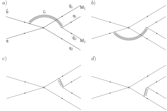
Figure 1: Feynman diagrams contributing to the amplitude of annihilation decay channels.

In this work we will compute non-leptonic B decays into two pseudoscalar mesons occurring only through annihilation diagrams. A typical decay is shown in Fig. 1, where the bottom quark decays via $W$ exchange or penguin processes, and a gluon that is emitted from any one of the quarks involved in the process creates a quark-antiquark pair in the final state, which will be a leading order process in $\alpha_{s}$. The channels we will analyze with these characteristics are:

• Charmless channels : $\bar{B}^{0}_{s}\to\pi^{+}\pi^{-}$; $\bar{B}^{0}_{d}\to K^{+}K^{-}$;

• Charmed channels: $\bar{B}_{d}^{0}\rightarrow D_{s}^{\pm}K^{\mp}$; $\bar{B}_{s}^{0}\rightarrow D^{\pm}\pi^{\mp}$.

To compute the annihilation amplitudes we use the QCDF approach, where the matrix elements are calculated through the Eq. (7). For the distribution amplitudes we adopt the expressions found on Ref.  beneke2 at leading twist order. The decay amplitude $\mathcal{A}(B\to M_{1}M_{2})$ is obtained from Eq. (6) and (7), and the branching ratio is then calculated from

$${\mathcal{B}}(B\to M_{1}M_{2})=\frac{\tau_{B}p_{c}}{8\pi m_{B}^{2}}|\mathcal{A}(B\to M_{1}M_{2})|^{2},$$ (9)

where $\tau_{B}$ is the $B$ meson lifetime and $p_{c}$ is the momentum of the final state particles with masses $m_{1}$ and $m_{2}$ in the $B$ meson rest frame, given by

$$p_{c}=\frac{\sqrt{(m_{B}^{2}-(m_{1}+m_{2})^{2})(m_{B}^{2}-(m_{1}-m_{2})^{2}))}}{2m_{B}}.$$ (10)

As mentioned before, these amplitudes contain divergences when dealt with in the collinear approximation, as in the QCDF approach. Such divergences can be eliminated in the pQCD method when the transverse momenta of the partons are taken into account pqcd -pqcd3 . However, in this work we will make use of non-perturbative gluon propagators, obtained with the help of SDE. These gluon propagators are finite in the infrared, and so they provide a natural cutoff to the singularities that appear in the collinear approximation. This kind of calculation has already been performed by Yang et al. yang -yangb for a specific SDE solution, and our intention is to make a more general discussion including other solutions, and verify how the results are dependent on the particular choices of SDE solutions. We also introduce the effect of the infrared finite coupling constant associated to each SDE solution, which was not considered in previous works.

III.1 Charmless channels

There are two charmless decay channels whose final states are light pseudoscalar mesons that occur through pure annihilation diagrams: $B_{s}^{0}$ $\to$ $\pi^{+}$ $\pi^{-}$ and $B_{d}^{0}$ $\to$ $K^{+}$ $K^{-}$. These channels happen through the elementary processes $b\bar{s}\to u\bar{u}$ and $b\bar{d}\to u\bar{u}$, respectively, and the creation of a $d\bar{d}$ pair by a gluon, as is shown in the Figs. 2a and 2b. These decays receive contributions from the $W$ exchange operator $Q_{2}$ and the penguin operators $Q_{4}$, $Q_{6}$, $Q_{8}$ and $Q_{10}$, given in the Eqs. (3)-(5), with $r=d$ and $r=s$ for the decays of the $B_{d}^{0}$ and $B_{s}^{0}$ mesons, respectively. The operators $Q_{2}$, $Q_{4}$ and $Q_{10}$ have a $(V-A)\otimes(V-A)$ structure while the operators $Q_{6}$ and $Q_{8}$ are of the type $(V-A)\otimes(V+A)$.

We compute the contribution of each operator for the diagrams of Fig. 1 with the help of Eq.(7). The diagrams that contribute for the amplitude are shown in Figs. 1a and 1b, since the contributions from the diagrams Figs. 1c and 1d cancel among themselves. The full amplitude for these decays is given by

$${\mathcal{A}}(B\to f) = \frac{G_{F}}{\sqrt{2}}f_{B}f_{M_{1}}f_{M_{2}}\pi\frac{C_{F}}{N_{C}^{2}}\,(V_{ub}\,V_{ur}^{*}\,{\mathcal{A}}_{\mathrm{Tree}}-V_{tb}\,V_{tr}^{*}\,{\mathcal{A}}_{\mathrm{Penguin}}),$$

with $r=d$ and $r=s$ for the decays of the $B_{d}^{0}$ and $B_{s}^{0}$ mesons, respectively. The tree level and penguin amplitudes are

$${\mathcal{A}}_{\mathrm{Tree}}=C_{2}\,A_{1}$$ (11)

and

$${\mathcal{A}}_{\mathrm{Penguin}}=\left(2\,C_{4}+\frac{C_{10}}{2}\right)\,A_{1}+\left(2\,C_{6}+\frac{C_{8}}{2}\right)\,A_{2}.$$ (12)

The functions $A_{1}$ and $A_{2}$ are the contributions from operators of the type $(V-A)\otimes(V-A)$ and $(V-A)\otimes(V+A)$, respectively, and are given by

$$A_{1} = \int_{0}^{1}d[X]\,\phi_{M_{1}}(x)\,\phi_{M_{2}}(y)\,\phi_{B}(z)\,D_{g}(x,y)\bigl{[}\alpha_{s}(\mu_{h})(y-z)D_{q}(x,y,z)+$$ (13)

$$+\alpha_{s}(\mu)(1-x)\,D_{b}(x,y,z)\bigr{]},$$

$$A_{2} = \int_{0}^{1}d[X],\phi_{M_{1}}(x)\,\phi_{M_{2}}(y)\phi_{B}(z)\,D_{g}(x,y)\bigl{[}\alpha_{s}(\mu_{h})\,(\bar{x}-z)\,D_{q}(x,y,z)+$$ (14)

$$+\alpha_{s}(\mu)\,y\,D_{b}(x,y,z)\bigr{]}\,,$$

where $d[X]=dx\,dy\,dz$, the quark propagators $D_{b}$ and $D_{q}$ ($q=d$ and $s$ for the $B_{d}^{0}$ and $B_{s}^{0}$ mesons, respectively) are given by:

$$D_{b}^{-1}(x,y,z) = (1-(x-z)(\bar{z}-y));$$

$$D_{q}^{-1}(x,y,z) = (\bar{x}-z)(y-z),$$

and $D_{g}(x,y)$ is the gluon propagator, whose the perturbative expression is $D_{g}^{-1}=k_{g}^{2}=y\,(1-x)$.

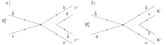
Figure 2: Quark contents of the decay channels: a) $B_{s}^{0}\to\pi^{+}\pi^{-}$, b) $B_{d}^{0}\to K^{+}K^{-}$.

The scales adopted in the calculations are $\mu=m_{b}$ for the contribution from the diagram shown in Fig. 1a where the gluon is emitted from the $b$ quark, and $\mu_{h}=\sqrt{\Lambda_{h}m_{b}}$ for the contribution shown in Fig. 1b where the gluon is emitted from the “spectator” quark, with $\Lambda_{h}=500$ MeV beneke2 . When the effective scale $\mu<m_{b}$ we use $\Lambda_{\mathrm{QCD}}=225$ MeV and when $\mu=m_{b}$ we use $\Lambda_{\mathrm{QCD}}=300$ MeV, and the difference is to match the values of the coupling constant due to different quarks thresholds. At the Eq. (III.1), the scales of the Wilson coefficients for each term are equal to the ones of the coupling constants.

III.2 Charmed channels

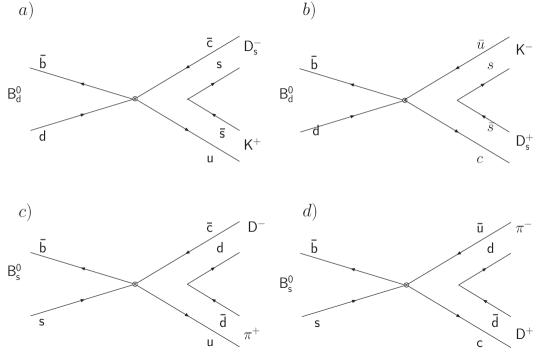
Figure 3: Quarks contents of the decay channels: a) $B_{d}^{0}$ $\rightarrow D_{s}^{-}K^{+}$, b) $B_{d}^{0}\rightarrow D_{s}^{+}K^{-}$, c) $B_{s}^{0}\rightarrow D^{-}\pi^{+}$, d) $B_{s}^{0}\rightarrow D^{+}\pi^{-}$

The charmed decay channels occur through $W$ exchange processes, and there is no contribution from penguin diagrams. The operators that contribute for the effective Hamiltonian are given by the current-current operators $Q_{1}$ and $Q_{2}$ (Eq. (2)). The Fig. 3a and 3b shows the quark diagrams for the decay channels $B_{d}^{0}\rightarrow D_{s}^{\mp}K^{\pm}$, which occur through the elementary processes $\bar{b}d\to\bar{c}u$ (or $\bar{b}u\to\bar{c}d$). The quark diagrams for the decay channel $B_{s}^{0}\rightarrow D^{\mp}\pi^{\pm}$ are shown in the Fig. 3c and 3d, occurring though the elementary process $\bar{b}s\to\bar{u}c$.

The full amplitude for the general processes $B^{0}\to D^{\mp}M^{\pm}$ (with $B=B_{d}$ and $B_{s}$, $D,M={D_{s},K},{D,\pi}$) will be calculated from

$${\mathcal{A}}(B^{0}\to D^{\mp}M^{\pm})=\frac{G_{F}}{\sqrt{2}}f_{B}f_{D}f_{M}\pi\frac{C_{F}}{N_{C}^{2}}V_{CKM}A_{B^{0}\to D^{\mp}M^{\pm}}\,,$$ (15)

The CKM factors for each decay channel are: $V_{\mathrm{CKM}}=V_{cb}^{*}V_{ud}$ for the $D_{s}^{-}K^{+}$ channel; $V_{ub}^{*}V_{cd}$ for $D_{s}^{+}K^{-}$; $V_{us}V_{cb}^{*}$ for $D^{-}\pi^{+}$ and $V_{cs}V^{*}_{ub}$ for $D^{+}\pi^{-}$. The functions $A_{{B^{0}\to D^{\mp}M^{\pm}}}$ are given by the following integrals:

$$A_{{B^{0}\to D^{-}M^{+}}} = \int_{0}^{1}{dx}\,{dy}\,{dz}\,\phi_{D}(y)\,\phi_{M}(x)\,D_{g}(x,y)\,\biggr{\{}\alpha_{s}(\mu_{f})\biggl{(}C_{1}(\mu_{f})+\frac{C_{2}(\mu_{f})}{2}\biggl{)}\times$$ (16)

$$\times [-(1-r^{2})\bigl{(}(1-2r^{2}-(1-r^{2})\,x)\,D_{c}(x)-y\,D_{u}(y)\bigr{)}\bigr{]}+\phi_{B}(z)\times$$

$$\times \bigl{[}\alpha_{s}(\mu_{h})\,C_{2}(\mu_{h})\,(1-r^{2})\,\bigl{(}(1-r^{2})\,(1-x)+r^{2}\,(y-z)\bigr{)}\,D_{d}(x,y,z)+$$

$$- \alpha_{s}(\mu)\,C_{2}(\mu)(1-r^{2})\,\bigl{(}(1+r^{2})\,(y+z)-r^{2}\bigr{)}\,D_{b}(x,y,z)\bigr{]}\biggr{\}}\,,$$

and

$$A_{B_{d}^{0}\to D^{+}M^{-}} = \int_{0}^{1}{dx}\,{dy}\,{dz}\,\phi_{D}(y)\,\phi_{M}(x)\,D_{g}(x,y)\biggr{\{}\alpha_{s}(\mu_{f})\biggl{(}C_{1}(\mu_{f})+\frac{C_{2}(\mu_{f})}{2}\biggl{)}\times$$ (17)

$$\times [(1-r^{2})\bigl{(}(1-2r^{2}-(1-r^{2})\,x)\,D_{c}(x)-\,y\,D_{u}(y)\bigr{)}\bigr{]}+\Phi_{B}(z)\times+$$

$$+ \bigl{[}\alpha_{s}(\mu_{h})C_{2}(\mu_{h})(1-r^{4})\,(y-z)\,D_{d}(x,y,z)-\alpha_{s}(\mu)C_{2}(\mu)(1-r^{2})\times$$

$$\times \bigl{(}(1-r^{2})\,(1-x)-r^{2}+r^{2}\,(y+z)\bigr{)}\,D_{b}(x,y,z)\bigr{]}\biggr{\}}\,.$$

The functions $D_{b}(x,y,z),\,D_{d}(x,y,z),\,D_{u}(y)$ and $D_{c}=D_{c}(x)$ are the quarks propagators, given by:

$$D_{b}^{-1}(x,y,z) = y+z+(1-y-z)(1-x)(1-r^{2});$$

$$D_{d}^{-1}(x,y,z) = x(z-y)(1-r^{2});$$

$$D_{c}^{-1}(x) = (1-x)(1-r^{2})\,;$$

$$D_{u}^{-1}(y) = y(1-r^{2})\,.$$

The function $D_{g}(x,y)$ is the gluon propagator, whose perturbative expression is $D_{g}^{-1}=k_{g}^{2}=y\,(1-x)\,(1-r^{2})$. Note that the integrals in the former equations (and also in Eqs. (13) and (14)) are dimensionless after the simplification of the $m_{B}$ dependence in both numerator and denominator.

The scales adopted in the calculations are the same as the charmless case: $\mu=m_{b}$ for the contribution of the diagram where the gluon is emitted from the $b$ quark, and $\mu_{h}=\sqrt{\Lambda_{h}m_{b}}$ for the contribution where the gluon is emitted from the “spectator” quark, with $\Lambda_{h}=500$ MeV. For the diagrams of Fig. 1c and 1d where the gluon is emitted from the quarks in the final state, we use the scale $\mu_{f}=\mu/2=m_{b}/2$. The QCD scales are also the same as the charmless case.

IV Non-perturbative gluon propagator and coupling constant

To compute the amplitudes discussed in the previous section, instead of the perturbative expression $D_{g}=(k^{2})^{-1}$ which is IR divergent, we will use for the gluon propagator $D_{g}(x,y)$ that appears in Equations (13), (14), (16) and (17) different solutions of the gluonic SDE obtained in the literature. Each one of these solutions is also associated to an infrared finite coupling constant that enters in the calculation. This coupling constant is evaluated at the scale $\mu$, which is the average energy of the gluon emission, where we may still have a small difference between the different solutions for the non-perturbative couplings. The propagators have the interesting property of being infrared finite eliminating the endpoint divergences, and at high energies they match with their perturbative counterpart. Note that, as discussed in Ref. natale , in these calculations we are integrating over the gluon propagator in a large region of the phase space, and this integration is weighted by different distribution functions, therefore the result will depend non-trivially on the formal expression of the propagator, as well as it will depend on different values of the non-perturbative coupling constant. Even with the large mass scale involved in the problem (the $B$ meson mass) we may expect a signal of the infrared behavior of these quantities.

Notice that the behavior of the coupling constant and the propagators are intimately connected. As shown by Cornall cornwall the product $g^{2}D(q^{2})$ is constant, in a more detailed discussion this can also be verified in the recent work by Aguilar and Papavassiliou aguilar2a ; aguilar2b ; aguilar08 . Furthermore Alkofer et al. in a series of papers alkofer -alkoferc have advocated that $\alpha_{s}(q^{2})=(g^{2}/4\pi)Z_{D}(q^{2})Z^{2}_{G}(q^{2})$ (the Z’ s are the gluon and ghost propagators dressing). Such type of relation is expected in the dynamical mass generation mechanism and can be traced back to the Slavnov-Taylor or Ward-type identities. Therefore the determination of the actual infrared behavior imply in the associated effect of the coupling constant and propagator!

It could be asked if there is double counting of non-perturbative dynamics between QCDF and the employment of infrared finite gluon propagators, since according to the factorization theorem, non-perturbative dynamics in B meson decay processes has been absorbed into distribution amplitudes. We stress that this is not the case. The effect of the infrared finite gluon propagators affects only the hard part of the hadronic matrix elements. The introduction of an infrared finite gluon propagator means that as we lower the energy we cannot neglect anymore the gluon dressing that is predicted by the SDE. Therefore dressed gluons provide the natural cutoff for the theory, and should be considered in the calculation as anticipated many years ago in the proposal of a dynamical perturbation theory by Pagels and Stokar pagels . Only the hard scattering kernels (like $T^{I}$ and $T^{II}$ in Eq.(6)) will be affected, and the distribution amplitudes should naturally contain the typical non-perturbative dynamics of the processes involving meson bound states.

The usual treatment of B meson decays involves consistent expansions in $\alpha_{s}$ and in $1/m_{b}$. Such level of consistency has not been achieved yet in the case of solutions of SDE for the gluon and fermion propagators. First, only quite recently it was developed a systematic gauge invariant approximation and truncation method for the gluonic Schwinger-Dyson equation (see the work of Ref. bp ). This method is consistent with an $\alpha_{s}$ expansion. Secondly, to also have an expansion consistent with a $1/m_{b}$ expansion for B meson decays it will be necessary to solve the coupled Schwinger-Dyson equations for the gluon and fermion propagators, and this is quite away from the present status of the theory. The only point that can be guessed at the moment is that the results for infrared finite gluon propagator will be only slightly changed by fermionic effects as far as the number of quarks remains equal to the known one.

In this section we present the different SDE solutions for the coupling constant and gluon propagator $(D(q^{2}))$. They were obtained as the result of different approximations made to solve the SDE for pure gauge QCD. There are two classes of solutions according to the behavior of the gluon propagator at the origin of the momenta, and both lead to an infrared frozen coupling constant: (a) an infrared finite gluon propagator which is different from zero at the origin of momenta, and (b) an infrared finite gluon propagator that goes to zero at the origin of momenta. Although the lattice simulations results definitely point out to an infrared finite propagator, there is no agreement about its behavior at $q^{2}=0$. A quite recent lattice argument favors a non zero value for $D(0)$ cucchieri .

The SDE solutions for the gluon propagator were obtained in different gauges as well as in a gauge independent approach. Here we just assume their validity for any gauge and write the propagator as

$$D_{\mu\nu}(q^{2})=\left(\delta_{\mu\nu}-\eta\frac{q_{\mu}q_{\nu}}{q^{2}}\right)D(q^{2})\,,$$ (18)

with $\eta=0$ in the Feynman gauge and $\eta=1$ in the Landau Gauge. In the following we briefly describe some of the solutions found in the literature.

IV.1 Infrared finite propagators with $D(0)\neq 0$

IV.1.1 Cornwall solution ⁴⁰

This solution was obtained by Cornwall many years ago and predicts a running coupling constant and gluon propagator which are infrared finite and non-null at the origin. It also predicts the existence of a dynamical gluon mass which is responsible for the infrared behavior of the aforementioned quantities. This dynamical gluon mass has a dependence on the momentum given by

$$M_{g}^{2}(q^{2})=m_{g}^{2}\left[\frac{\mathrm{ln}\left(\frac{q^{2}+4m_{g}^{2}}{\Lambda^{2}}\right)}{\mathrm{ln}\left(\frac{4m_{g}^{2}}{\Lambda^{2}}\right)}\right]^{-\frac{12}{11}},$$ (19)

where $m_{g}$ is the gluon mass scale and $\Lambda=\Lambda_{\mathrm{QCD}}$ is the QCD scale. The running coupling constant is

$$\alpha_{\mathrm{s}}^{\mathrm{Ia}}(q^{2})=\frac{4\pi}{\beta_{0}\mathrm{ln}\left(\frac{q^{2}+4M_{g}^{2}(q^{2})}{\Lambda^{2}}\right)},$$ (20)

with $\beta_{0}=11-\frac{2}{3}n_{f}$, and $n_{f}$ is the number of active quark flavors at a given scale. Although the SDE were solved for the pure gauge theory it is usually assumed that their solutions will not be strongly affected by the introduction of fermions as long as $n_{f}$ is not too large natale3 ; natale4 . The gluon propagator is equal to

$$D_{\mathrm{Ia}}(q^{2})=\frac{1}{\left[q^{2}+M_{g}^{2}(q^{2})\right]\beta_{0}g^{2}\ln\left(\frac{q^{2}+4M_{g}^{2}(q^{2})}{\Lambda^{2}}\right)}\,,$$ (21)

where the parameter $g^{2}$ is the strong coupling given by $\alpha_{s}=g^{2}/4\pi$. The dynamical gluon mass $m_{g}$ has typical values natale3 -natale5 ; cornwall :

$$m_{g}=500\pm 200\,\mathrm{MeV}\,\,\,.$$ (22)

IV.1.2 Fit of Ref. 50

Another solution with a dynamical gluon mass was found in Ref. aguilar1 . This solution was fitted by the simplest way to have a dynamically massive gluon, whose mass obeys the standard OPE behavior at high energy ($m_{g}^{2}(q^{2})\propto m_{0}^{4}/q^{2}$)

$$D_{\mathrm{IIa}}(q^{2})=\frac{1}{q^{2}+M^{2}(q^{2})},$$ (23)

with $m_{0}$ being the gluon mass scale, and $M^{2}(q^{2})$ the dynamical gluon mass given by

$$M^{2}(q^{2})=\frac{m_{0}^{4}}{q^{2}+m_{0}^{2}}.$$ (24)

The coupling constant is similar to the previous solution, with $M_{g}(q^{2})$ being replaced by $M^{2}(q^{2})$.

IV.1.3 Aguilar-Papavassiliou solution ^51,52

The SDE solution obtained by Aguilar and Papavassiliou results from a quite detailed analysis of the gluon propagator using the pinch technique, which maintains the desirable property of transversality of the propagator. This solution is represented by

$$D_{\mathrm{IIc}}(q^{2})=\frac{1}{q^{2}+m^{2}(q^{2})}\,.$$ (25)

The dynamical mass is:

$$m^{2}(q^{{}^{2}})=\frac{m_{0}^{4}}{q^{2}+m_{0}^{2}}\left[\ln\left(\frac{q^{2}+\rho m^{2}_{0}}{\Lambda^{2}}\right)/\ln\left(\frac{\rho m_{0}^{2}}{\Lambda^{2}}\right)\right]^{\gamma_{2}-1}\,,$$ (26)

with $\gamma_{2}>1$. The running coupling constant is given by

$$g^{2}(q^{2})=\left[\beta_{0}\ln\left(\frac{q^{2}+f(q^{2},m^{2}(q^{2}))}{\Lambda^{2}}\right)\right]^{-1}\,,$$ (27)

where the function $f(q^{2},m^{2}(q^{2}))$ is given by a power law expression

$$f(q^{2},m^{2}(q^{2})) = \rho_{1}m^{2}(q^{2})+\rho_{2}\frac{m^{4}(q^{2})}{q^{2}+m^{2}(q^{2})}+\rho_{3}\frac{m^{6}(q^{2})}{[q^{2}+m^{2}(q^{2})]^{2}}\,.$$ (28)

The parameters $\rho$, $\rho_{1}$, $\rho_{2}$, $\rho_{3}$ and $\gamma_{2}$ are fitted numerically. For $\Lambda=300$ MeV and $m_{0}=250\,\mathrm{MeV}$ the numerical values of the parameters are the following: $\rho=2.47$, $\gamma_{2}=1.76$ $\rho_{1}=5.615$, $\rho_{2}=-8.523$, $\rho_{3}=3.584$; and for $m_{0}=600\,\mathrm{MeV}$ the parameters are: $\rho=1.234$, $\gamma=1.64$, $\rho_{1}=2.894$, $\rho_{2}=-4.534$, $\rho_{3}=2.043$.

The Fig. 4 shown the behavior of the propagators and coupling constants of the three solutions presented in this subsection.

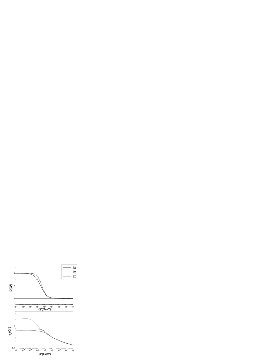
Figure 4: Coupling constants and propagators for the three solutions with infrared finite propagators and $D(0)\neq 0$, with $m_{g}=m_{0}=500$ MeV: (Ia) Cornwall solution, (Ib) solution of Ref. 50, (Ic) Aguilar-Papavassiliou solution.

IV.2 Infrared finite propagators with $D(0)=0$

IV.2.1 Alkofer et al. solution ⁵³

This solution, obtained in the Landau gauge, has a different qualitative behavior relative to the ones we have presented so far. Although this solution also predicts a freezing of the coupling constant, and the solution for the gluon propagator is also infrared finite, the propagator vanishes at the origin of momenta. The behavior of the running coupling constant is given by

$$\alpha_{\mathrm{s}}^{\mathrm{IIa}}(q^{2})=\frac{\alpha_{A}(0)}{\ln[e+a_{1}(q^{2})^{a_{2}}+b_{1}(q^{2})^{b2}]}\,,$$ (29)

and the propagator is equal to

$$D_{\mathrm{IIa}}(q^{2})=\frac{Z(q^{2})}{q^{2}}\,,$$ (30)

where $Z(q^{2})$ and $R(q^{2})$ are fitted as

$$Z(q^{2})=\left(\frac{\alpha_{\mathrm{sA}}(q^{2})}{\alpha_{\mathrm{sA}}(\mu)}\right)^{1+2\delta}R^{2}(q^{2})\,,$$ (31)

and

$$R(q^{2})=\frac{c(q^{2})^{\kappa}+d(q^{2})^{2\kappa}}{1+c(q^{2})^{\kappa}+d(q^{2})^{2\kappa}}\,.$$ (32)

The constants are parameters obtained in the fitting of the SDE numerical solution:

$\alpha_{A}(0)=2.972$, $\alpha_{\mathrm{sA}}(\mu)=0.9676$, $a_{1}=5.292\,\mathrm{GeV}^{-2a_{2}}$,

$b_{1}=0.034\,\mathrm{GeV}^{-2b_{2}}$, $a_{2}=2.324$, $b_{2}=3.169$,

$\kappa=0.5953$, $\delta=-9/4$, $c=1.8934$ GeV^-2κ,

$d=4.6944$ GeV${}^{-4\kappa}.$

IV.2.2 Fit of Ref. 54

A more recent fit obtained by Alkofer et al. alkofer2 ; alkoferc , resulting from different approximations for the SDE, leads to the following expression for the function $Z(q^{2})$ that appears in the equation (30)

$$Z_{\mathrm{fit}}(q^{2})=w\left(\frac{q^{2}}{q^{2}+\Lambda^{2}}\right)^{2\kappa}(\alpha_{\mathrm{fit}}(q^{2}))^{-\gamma}\,,$$ (33)

where $\gamma=(-13N_{C}+4n_{f})/(22N_{C}-4n_{f})$. The the parameter $w$ comes from the normalization of the function $Z(p^{2})$ as $Z(p^{2}=1GeV)=1$, giving $w=1.32$ for $\Lambda=300$ MeV and $w=1.4$ for $\Lambda=225$ MeV. The propagator for this solution is then

$$D_{\mathrm{IIb}}(q^{2})=\frac{Z_{\mathrm{fit}}(q^{2})}{q^{2}}\,,$$ (34)

and the running coupling constant is given by

$$\alpha_{\mathrm{fit}}(q^{2})=\frac{\alpha_{S(0)}}{1+q^{2}/\Lambda^{2}}+\frac{4\pi}{\beta_{0}}\frac{q^{2}}{q^{2}+\Lambda^{2}}\times\bigg{(}\frac{1}{\ln(q^{2}/\Lambda^{2})}-\frac{1}{q^{2}/\Lambda^{2}-1}\bigg{)}\,,$$

with $\beta_{0}=(11N_{C}-2n_{f})/3$.

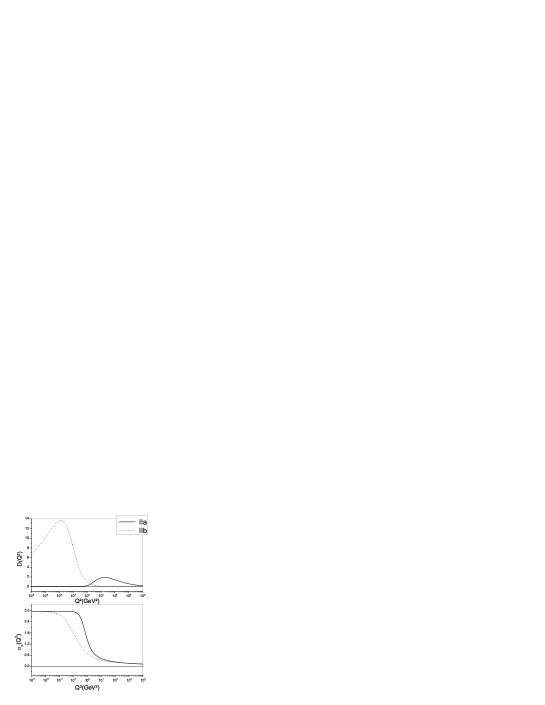
Figure 5: Coupling constants and propagators for the two solutions with infrared null propagators: (IIa) Alkofer et al. solution, (IIb) solution of Ref. 51.

The Fig. 5 shows the behavior of the propagators and coupling constants of the two solutions presented in this subsection.

V Numerical results

In the numerical calculations we use the asymptotic expression for the wave functions of the light mesons, pions and kaons,

$$\Phi_{\pi,K}(x)\,=\,6\,x\,(1-x),$$ (35)

while for the $D$ mesons we use

$$\Phi_{D}(x)\,=\,6\,x\,(1-x)\,[1+a_{D}(1-2x)],$$ (36)

with $a_{D}=0.8$ for $D^{\pm}$ and $a_{D}=0.3$ for the $D_{s}^{\pm}$ meson lu1 ; lu2 . We neglected the momentum of the “spectator” quark in the calculation, i.e. we assume $x,y\gg z$, and in this approximation the distribution amplitude for the $B$ meson is given by a delta function. Some results will also be presented in the case where the wave functions of light mesons are represented by an expansion in Gegenbauer polynomials. The Wilson coefficients are computed using the equations given in the appendices of Ref. wilson . We do not include strong phases in the calculation of the integrals, i.e. our amplitudes will be real apart from CKM phases. It is known that the strong phases generated by the annihilation amplitudes are crucial for predicting CP asymmetries. For example, in the Ref. yangb the strong phases of annihilation amplitudes are generated by applying the Cutkosky rules for the quark propagators. However, the asymmetries are obtained from the ratio of amplitudes and the CP asymmetry parameters are not sensitive to the cutoff effect (or the infrared finite gluon propagator). Moreover the main theoretical errors originate from the CKM parameters yangb .

We also use the following parameters pdg :

• Masses:

  $m_{B_{d}}=5.28$ GeV, $m_{B_{s}}=5.37$ GeV, $m_{D}=1.87$ GeV, $m_{D_{s}}=1.97$ GeV, $m_{b}=4.7$ GeV;

• Decay constants:

  $f_{B_{d}}=0.200$ GeV, $f_{B_{s}}=0.236$ GeV, $f_{D}=0.226$ GeV, $f_{D_{s}}=0.241$ GeV, $f_{\pi}=0.132$ GeV, $f_{K}=0.160$ GeV;

• Lifetimes:

  $\tau_{B_{d}}=1.54$ ps, $\tau_{B_{s}}=1.466$ ps;

• CKM parameters:

  $A=0.818$, $\lambda=0.2272$, $\bar{\rho}=0.221$, $\bar{\eta}=0.340$.

The Table 1 shows the branching ratios obtained for each decay channel for the different propagators and coupling constants discussed in the previous section. As we shall detail in the conclusions, it is possible to see that the non-leptonic $B$ decays resulting from annihilation channels are sensitive to the infrared QCD behavior.

Table 1: Branching ratios $\mathcal{B}$ for decays of the $B$ meson obtained with the different infrared finite gluon propagators and coupling constants, and with $m_{g}=m_{0}=500$ MeV and $\mu=m_{b}$: Cornwall (Ia), Ref. 50 (Ib), Aguilar-Papavassiliou (Ic), Alkofer et al. (IIa), Ref. 54 (IIb). We use $\Lambda_{\mathrm{QCD}}=225$ Mev, for $\mu\leq m_{b}$ and $\Lambda_{\mathrm{QCD}}=300$ Mev, for $\mu>m_{b}$. The experimental data for the branching ratios of the decay channels are also shown, and the corresponding references.

${\mathcal{B}}$(Decay channel)	$D_{Ia}$	$D_{Ib}$	$D_{Ic}$	$D_{IIa}$	$D_{IIb}$	Experimental data	Ref.
${\mathcal{B}}(B_{s}^{0}$$\rightarrow$ $\pi^{+}\pi^{-})$$\times$$10^{7}$	1.08	1.58	1.02	4.30	3.73	$<17$	cdf1
						$<13.6$	cdf2
${\mathcal{B}}(B_{d}^{0}$$\rightarrow$$K^{+}K^{-})$$\times$$10^{8}$	4.92	7.18	4.63	19.62	16.90	$9^{+18}_{-13}{\pm}1$	belle
						$<37$	pdg
						$4{\pm}15{\pm}8$	babar
${\mathcal{B}}(B_{s}^{0}$$\rightarrow$$D^{-}\pi^{+})$$\times$$10^{6}$	1.03	1.54	0.99	4.40	4.02	–	–
${\mathcal{B}}(B_{s}^{0}$$\rightarrow$$D^{+}\pi^{-})$$\times$$10^{7}$	1.28	1.88	1.22	5.31	4.76	–	–
${\mathcal{B}}(B_{d}^{0}$$\rightarrow$$D_{s}^{-}K^{+})$$\times$$10^{5}$	1.34	1.98	1.27	5.61	3.72	$4.6^{+1.2}_{-1.1}{\pm}1.0$	belle2
						$3.2\pm 1.0\pm 1.0$	babar2
						$3.1\pm 0.8$	pdg
${\mathcal{B}}(B^{0}_{d}$$\rightarrow$$D_{s}^{+}K^{-})$$\times$$10^{8}$	0.67	0.99	0.64	2.66	1.79	$<1.1\times 10^{5}$	pdg

VI Conclusions

We have studied some decay channels of $B^{0}_{s}\,(\bar{B}^{0})$ and $B^{0}_{d}\,(\bar{B}_{d}^{0})$ mesons which occur through the annihilation diagrams: $B_{s}^{0}\to\pi^{+}\pi^{-},\,D^{\pm}\pi^{\mp}$ and $B_{d}^{0}\to K^{+}K^{-},\,D_{s}^{\pm}K^{\mp}$. We have argued that infrared finite gluon propagators and running coupling constants obtained as solutions of the QCD Schwinger-Dyson equations, may serve as a natural cutoff for the end-point divergences that appear in the calculation of these decays.

We computed several branching ratios for some of the different solutions of gluon propagators and coupling constants found in the literature. These different solutions appear due to different approximations performed to solve the SDE. Our results are shown in Table 1. We argue that a systematic study of $B$ decays may help to give information about the infrared QCD behavior. Note that the results of Table 1 are not trivial, in the sense that the differences in the branching ratios come out from the integration over different expressions for the gluon propagators multiplied by different wave functions. It is possible to see in Table 1 that the different classes of gluon propagators, according to its infrared behavior, lead to branching ratios differing by a factor of approximately 2 to 4. The existing experimental data of the decay channels that we have discussed is shown in Table 1. The experimental data, when confronted with the results of Table 1, may already be used to claim that some approximations to solve the SDE of pure gauge QCD lead to poor predictions for some of the branching ratios (see, for instance, the results related to the propagator indicated by $D_{IIa}$).

In the calculation of B mesons decays through the factorization theorems, the dominant sources of theoretical uncertainties are the mesons wave functions and the scale parameter $\mu$, as has been pointed out in Ref. beneke2 . We have analyzed these uncertainties in our calculations for the decay channel $B^{0}_{s}\to D^{-}_{s}K^{+}$ and our results are shown in Table 2, and as we shall see in the sequence all these uncertainties are less important than the differences originated by the two classes of gluon propagators. We can see that the branching ratios are not very sensitive to the shape of the wave functions, with a difference of about 2% between the results using the asymptotic function and the expansion in Gegenbauer polynomials, which is much below the present experimental accuracy. The main source of uncertainty is the scale parameter, with a variation of about 40-60%. This strong dependence is expected since the annihilation decay processes are of ${\mathcal{O}}(\alpha_{s}(\mu))$ in the perturbative expansion. This dependence can be reduced considering higher order terms of the perturbative expansion. Once the uncertainties in these quantities become well known we certainly will be able to extract information on the gluon mass parameter. It is important to notice that the amplitude that we calculate for each specific decay is a convolution of the gluon propagator and coupling constant with the wave functions of the final state mesons, therefore the result is peaked at different momenta, depending on the meson masses, and help to discriminate the form of the gluon propagator and infrared coupling constant. Actually, this is the reason for the different sensitivities on the IR cutoff in the decay channels discussed in this work, which will help to eliminate the possible uncertainties. It should also be remembered that the next order twist can modify the results, but if we have a large confidence level in the values of these many parameters or functions, we certainly can test the infrared QCD behavior in these decays. In Table 2 it is also evident the differences between using SDE solutions of the type I and II for the propagators and coupling constants.

Table 2: Branching ratios for the decay channel $B^{0}_{s}\to D^{-}_{s}K^{+}$, ${\mathcal{B}}(B_{d}^{0}\rightarrow D_{s}^{-}K^{+})\times 10^{5}$. We compare two different scales, $\mu=m_{b}$ and $\mu=m_{b}/2$, and use the asymptotic wave function of the $K$ meson and also the wave function expanded in Gegenbauer polynomials (at the scale $\mu=m_{b}$, with $\alpha_{1}(1\,{\mathrm{GeV}})=0.17$ and $\alpha_{2}(1\,{\mathrm{GeV}})=0.2$, Ref. 56). We also show the results for different gluon masses.

	Asymptotic		Gegenbauer
Gluon propagators	$\mu=m_{b}$	$\mu=m_{b}/2$	$\mu=m_{b}$
$D_{Ia}$, $m_{g}=400$ MeV	1.95	3.25	2.00
$D_{Ia}$, $m_{g}=500$ MeV	1.34	2.09	1.36
$D_{Ib}$, $m_{0}=400$ MeV	2.70	4.89	2.75
$D_{Ib}$, $m_{0}=500$ MeV	1.98	3.48	2.02
$D_{Ic}$, $m_{0}=500$ MeV	1.84	3.10	1.87
$D_{Ic}$, $m_{0}=600$ MeV	1.40	2.40	1.41
$D_{IIa}$	5.61	16.78	5.75
$D_{IIb}$	3.72	7.32	3.95

It is clearly necessary to collect much more data to settle the question about the infrared QCD behavior, at least in what concerns the infrared behavior of the gluon propagator and coupling constant. We know that the comparison with the experimental data will also depend on quantities like the distribution functions, but with the LHCb experiment the uncertainty in the experimental data will be narrowed, and it will be possible to explore different models until a reasonable physical picture of the $B$ meson decays is obtained.

From the tables shown above we see that the results depend sensitively on the different solutions of infrared finite gluon propagators. It must be said that a lot of progress has been done in the subject of SDE for the gluon propagators recently, this also happened to attract the attention of lattice researchers, and we believe that the lattice simulation of the gluon propagator can only be fitted nicely by the “massive gluon solution”, see for instance Ref. aguilar08 , although this is not an unanimous opinion. If with improved lattice results we come to the conclusion that the massive gluon propagator is the one chosen by Nature, we verify that the theoretical uncertainty will be only due to the poor knowledge of the gluon mass value. In this case we can see from our results that the variation of the branching ratios is not so large, and will be smaller as long as this gluon mass is better determined through all its phenomenological consequences.

In order to fully understand the non-leptonic $B$ decays that we discussed in this work we see two specific directions of study. One of these is the need of finding a gauge invariant truncation in the context of the SDE. The importance of constructing such a truncation scheme is the possibility of defining a non-perturbative effective charge for QCD, which constitutes a generalization in a non-abelian theory of the QED effective charge as discussed in Ref. bp . If this step was accomplished in all its glory, it would be possible discard one of the solutions of the infrared sector of QCD on the basis of gauge-invariance. The other direction of study is that there should be a systematic use of infrared finite gluon propagators and coupling constant in non-leptonic $B$ meson decays. Any $B$ meson decay involving a gluon exchange will be affected by the IR cutoff that we discussed here, and we intend to study other decays as well as to implement the higher twist effects in this calculation. The infrared finite gluon propagator provides a natural cutoff for these phenomenological processes. As we have seen in Table 1, the branching ratios of heavy mesons depend on the infrared QCD details, and this will certainly happen when we have light mesons in the final states. The most remarkable result of Table 1 is that with the concept of a dynamically massive gluon it is possible to predict the branching ratios of some $B$ decays compatible with the experimental data, without the help of any ad hoc cutoff and with the same mass scale that fits the experimental data of many other processes.

References

- (1) M. Wirbel, B. Stech, and B. Manfred, Z. Phys. C29, 637 (1985).
- (2) M. Bauer, B. Stech, and M. Wirbels, Z. Phys. C34, 103 (1987).
- (3) L. L. Chau, H. Y. Cheng, W. K. Sze, H. Yao, and B. Tseng, Phys. Rev. D43, 2176 (1991).
- (4) A. Szczepaniak, E. M. Henley, and S. J. Brodsky, Phys. Lett. B243, 287 (1990).
- (5) G. P. Lepage and S. J. Brodsky, Phys. Lett. B87, 359 (1979).
- (6) G. P. Lepage and S. J. Brodsky, Phys. Rev. D22, 2157 (1980).
- (7) J. Botts and G. Sterman, Nucl. Phys. B325, 62 (1989).
- (8) H.-N. Li and G. Sterman, Nucl. Phys. B381, 129 (1992).
- (9) M. Beneke, G. Buchalla, M. Neubert, and C. T. Sachrajda, Phys. Rev. Lett. 83, 1914 (1999), eprint hep-ph/9905312.
- (10) M. Beneke, G. Buchalla, M. Neubert, and C. T. Sachrajda, Nucl. Phys. B591, 313 (2000), eprint hep-ph/0006124.
- (11) M. Beneke, G. Buchalla, M. Neubert, and C. T. Sachrajda, Nucl. Phys. B606, 245 (2001), eprint hep-ph/0104110.
- (12) M. Beneke and M. Neubert, Nucl. Phys. B675, 333 (2003), eprint hep-ph/0308039.
- (13) G. Buchalla, A. J. Buras, and M. E. Lautenbacher, Rev. Mod. Phys. 68, 1125 (1996), eprint hep-ph/9512380.
- (14) A. A. Natale, Braz. J. Phys. 37, 306 (2007), eprint hep-ph/ 0610256.
- (15) D. Binosi and J. Papavassiliou (2007), eprint arXiv:0712.2707 [hep-ph].
- (16) A. Cucchieri and T. Mendes (2007a), eprint arXiv:0710.0412 [hep-lat].
- (17) I. L. Bogolubsky, E. M. Ilgenfritz, M. Muller-Preussker, and A. Sternbeck (2007), eprint arXiv:0710.1968 [hep-lat].
- (18) A. Cucchieri and T. Mendes (2007b), eprint arXiv:0712.3517 [hep-lat].
- (19) F. Halzen, G. I. Krein, and A. A. Natale, Phys. Rev. D47, 295 (1993).
- (20) M. B. G. Ducati, F. Halzen, and A. A. Natale, Phys. Rev. D48, 2324 (1993), eprint hep-ph/9304276.
- (21) A. C. Aguilar, A. Mihara, and A. A. Natale, Phys. Rev. D65, 054011 (2002), eprint hep-ph/0109223.
- (22) A. Mihara and A. A. Natale, Phys. Lett. B482, 378 (2000), eprint hep-ph/0004236.
- (23) A. C. Aguilar, A. Mihara, and A. A. Natale, Int. J. Mod. Phys. A19, 249 (2004).
- (24) E. G. S. Luna, A. F. Martini, A. M. M. J. Menon, and A. A. Natale, Phys. Rev. D72, 034019 (2005), eprint hep-ph/0507057.
- (25) E. G. S. Luna and A. A. Natale, Phys. Rev. D73, 074019 (2006), eprint hep-ph/0602181.
- (26) F. Carvalho, A. A. Natale, and C. M. Zanetti, Mod. Phys. Lett. A21, 3021 (2006), eprint hep-ph/0510172.
- (27) E. G. S. Luna, A. A. Natale, and C. M. Zanetti, Int. J. Mod. Phys. A23, 151 (2008), eprint hep-ph/0605338.
- (28) S. J. Brodsky, C. R. Ji, A. Pang, and D. G. Robertson, Phys. Rev. D57, 245 (1998), eprint hep-ph/9705221.
- (29) D. V. Shirkov and I. L. Solovtsov, Phys. Rev. Lett. 79, 1209 (1997), eprint hep-ph/9704333.
- (30) A. C. Aguilar, A. V. Nesterenko, and J. Papavassiliou, J. Phys. G31, 997 (2005), eprint hep-ph/0504195.
- (31) A. V. Nesterenko and J. Papavassiliou, Int. J. Mod. Phys. A20, 4622 (2005a), eprint hep-ph/0409220.
- (32) A. V. Nesterenko and J. Papavassiliou, Phys. Rev. D71, 016009 (2005b), eprint hep-ph/0410406.
- (33) A. C. Aguilar, A. A. Natale, and P. S. R. da Silva, Phys. Rev. Lett. 90, 152001 (2003), eprint hep-ph/0212105.
- (34) H. Pagels and S. Stokar, Phys. Rev. D20, 2947 (1979).
- (35) S. J. Brodsky, E. Gardi, G. Grunberg, and J. Rathsman, Phys. Rev. D63, 094017 (2001), eprint hep-ph/0002065.
- (36) S. J. Brodsky, C. M. S. Menke, and J. Rathsman, Phys. Rev. D67, 055008 (2003), eprint hep-ph/0212078.
- (37) J. M. Cornwall, Phys. Rev. D76, 025012 (2007), eprint hep-th/ 0702054.
- (38) S. J. Brodsky, Acta Phys. Polon. B32, 4013 (2001), eprint hep-ph/0111340.
- (39) S. J. Brodsky, Fortsch. Phys. 50, 503 (2002), eprint hep-th/ 0111241.
- (40) J. M. Cornwall, Phys. Rev. D26, 1453 (1982).
- (41) S. Bar-Shalom, G. Eilam, and Y. D. Yang, Phys. Rev. D67, 014007 (2003), eprint hep-ph/0201244.
- (42) Y. D. Yang, F. Su, G. R. Lu, and H. J. Hao, Eur. Phys. J. C44, 243 (2005), eprint hep-ph/0507326.
- (43) Y. L. W. F. Su, Y. D. Yang, and C. Zhuang, Eur. Phys. J. C48, 401 (2006), eprint hep-ph/0604082.
- (44) H. N. Li and H. L. Yu, Phys. Rev. Lett. 74, 4388 (1995a), eprint hep-ph/9409313.
- (45) H. N. Li and H. L. Yu, Phys. Lett. B353, 301 (1995b).
- (46) Y. Y. Keum, H. N. Li, and A. I. Sanda, Phys. Rev. D63, 054008 (2001), eprint hep-ph/0004173.
- (47) H. N. Li, Phys. Rev. D52, 3958 (1995), eprint hep-ph/9412340.
- (48) C.-D. Lu and K. Ukai, Eur. Phys. J. C28, 305 (2003), eprint hep-ph/0210206.
- (49) Y. Li and C.-D. Lu, Commun. Theor. Phys. 44, 659 (2005), eprint hep-ph/0502038.
- (50) A. C. Aguilar and A. A. Natale, JHEP 08, 057 (2004), eprint hep-ph/0408254.
- (51) A. C. Aguilar and J. Papavassiliou, JHEP 12, 012 (2006), eprint hep-ph/0610040.
- (52) A. C. Aguilar and J. Papavassiliou (2007), eprint arXiv: 0708.4320 [hep-ph].
- (53) C. S. Fischer, R. Alkofer, and H. Reinhardt, Phys. Rev. D65, 094008 (2002), eprint hep-ph/0202195.
- (54) R. Alkofer and L. von Smekal, Phys. Rept. 353, 281 (2001), eprint hep-ph/0007355.
- (55) R. Alkofer, C. S. Fischer, F. J. Llanes-Estrada, and K. Schwenzer, POS LAT2007, 286 (2007), eprint arXiv:0710.1154 [hep-ph].
- (56) P. Ball, JHEP 09, 005 (1998), eprint hep-ph/9802394.
- (57) K. Abe et al. (Belle), Phys. Rev. Lett. 98, 181804 (2007), eprint hep-ex/0608049.
- (58) W. M. Yao et al. (Particle Data Group), J. Phys. G33, 1 (2006).
- (59) B. Aubert et al. (BABAR) (2005), eprint hep-ex/0508046.
- (60) A. Abulencia et al. (CDF), Phys. Rev. Lett. 97, 211802 (2006), eprint hep-ex/0607021.
- (61) M. Morello (CDF), Nucl. Phys. Proc. Suppl. 170, 39 (2007), eprint hep-ex/0612018.
- (62) P. Krokovny et al. (Belle), Phys. Rev. Lett. 89, 231804 (2002), eprint hep-ex/0207077.
- (63) B. Aubert et al. (BABAR), Phys. Rev. Lett. 90, 181803 (2003), eprint hep-ex/0211053.
- (64) C. D. Lu, K. Ukai, and M. Z. Yang, Phys. Rev. D63, 074009 (2001), eprint hep-ph/0004213.
- (65) A. C. Aguilar, D. Binosi, and J. Papavassiliou (2008), eprint arXiv:0802.1870 [hep-ph].