Vortices, circumfluence, symmetry groups and Darboux transformations of the (2+1)-dimensional Euler equation

Abstract

The Euler equation (EE) is one of the basic equations in many physical fields such as fluids, plasmas, condensed matter, astrophysics, oceanic and atmospheric dynamics. A symmetry group theorem of the (2+1)-dimensional EE is obtained via a simple direct method which is thus utilized to find exact analytical vortex and circumfluence solutions. A weak Darboux transformation theorem of the (2+1)-dimensional EE can be obtained for arbitrary spectral parameter from the general symmetry group theorem. Possible applications of the vortex and circumfluence solutions to tropical cyclones, especially Hurricane Katrina 2005, are demonstrated.

I Introduction.

There are various important open problems in fluid physics. One of the most important problems is the existence and smoothness problem of the Navier-Stokes (NS) equation. The NS equation has been recognized as the basic equation and the very starting point of all problems in fluid physics NS . Due to its importance and difficulty, it is listed as one of the millennium problems of the 21st century clay .

One of the most significant recent developments related to the above problem may be the discovery of Lax pairs of two- and three- dimensional Euler equations (EEs) which are the limit cases of the NS equation for a large Reynolds number Li ; Li1 . Actually, for the two-dimensional EE, the Lax pair given in Li ; Li1 is weak (see Remark 2 of the next section) while the Lax pairs of the three-dimensional EE are strong (see Theorems 3 and 4 of LTJH which can be proved in a similar way as Theorem 1 of this paper). Hence, the EEs are (weak) Lax integrable under the meaning that they possess (weak) Lax pairs, and subsequently the NS equations with large Reynolds number are singular perturbations of (weak) Lax-integrable models.

The (3+1)-dimensional EE

$$E_{1} \equiv \vec{\omega}_{t}+(\vec{u}\cdot\nabla)\vec{\omega}-(\vec{\omega}\cdot\nabla)\vec{u}=0,$$ (1)

$$\vec{\omega} = \nabla\times\vec{u},\$$ (2)

with $\vec{\nabla}\cdot\vec{u}=0$ is the original springboard for investigating incompressible inviscid fluid. In Eqs. (1) and (2), $\vec{\omega}\equiv\{\omega_{1},\ \omega_{2},\ \omega_{3}\}$ is the vorticity and $\vec{u}\equiv\{u_{1},\ u_{2},\ u_{3}\}$ is the velocity of the fluid.

In (2+1)-dimensional case, the EE has the form of

$$E\equiv\omega_{t}+[\psi,\omega]=0,\qquad\omega = \psi_{xx}+\psi_{yy},$$ (3)

where the velocity $\vec{u}=\{u_{1},\ u_{2}\}$ is determined by the stream function $\psi$ through

$$u_{1}=-\psi_{y},\ u_{2}=\psi_{x}$$ (4)

and the Jacobian operator (or, namely, commutator) $[A,\ B]$ is defined as

$$[A,\ B]\equiv A_{x}B_{y}-B_{x}A_{y}.$$ (5)

It is known that the EEs are important not only in fluid physics fluid but also in many other physical fields such as plasma physics plasma , oceanography ocean , atmospheric dynamics gas , superfluid and superconductivity super , cosmography and astrophysics astro , statistical physics sta , field and particle physicsparticle and condensed matter including Bose-Einstein condensation bose , crystal liquid crystal and liquid metallic hydrogen H , etc..

As a beginning point of various physical problems, the EEs have been studied extensively and intensively, which is manifested by a large number of related papers on EEs in the literature. For instance, a lot of exact analytical solutions of the EEs have been presented, some of which can be found in the classical book of H. Lamb Lamb . In Sov , the authors studied the planar rotational flows of an ideal fluid and the addressing method was developed to obtain exact solutions of the EEs in Yu . In addition, some types of exact solutions were obtained via a Bäcklund transformation in Jia . However, rather few exact analytic solutions of the EEs have been obtained from the (weak) Lax pair since it was revealed by Charles Li Li around five years ago. A special type of Darboux transformation (DT) with zero spectral parameter for the (2+1)-dimensional EE was shown in Li , and some types of DTs (or weak DTs) with nonzero spectral parameter(s) for both (2+1)- and (3+1)-dimensional EEs were presented in our unpublished paper LTJH .

Lie group theory is one of the most effective methods of seeking exact and analytic solutions of physical systems. However, even for a mathematician, it is still rather difficult to find a symmetry group, especially non-Lie and non-local symmetry groups. So for physicists, it would be more significant and meaningful to establish a simple method to obtain more general symmetry groups of nonlinear systems without using complicated group theory.

To our knowledge, there is little exact analytic understanding of the vortices and circumfluence, although they are most general observations in some physical fields; in particular, very rich vortex structures exist in fluid systems. In fact, if one could find the full symmetry groups of the EEs, then many kinds of exact vortex and circumfluence solutions could be generated from some simple trivial solutions.

This paper is an enlarged version of our earlier, unpublished paper LTJH . In section II, we first establish a simple direct method to find a general group transformation theorem for the (2+1)-dimensional EE, then utilize the theorem in some special cases to obtain some solution theorems which lead to a quite general symmetric vortex solution with some arbitrary functions. The applications of the exact vortices and circumfluence solutions are given in section III. It is indicated that the solutions can explain the tropical cyclone (TC) eye, the track, and the relation between the track and the background wind. The TC tracks can thus be predicted by the relation. In section IV, beginning with a general symmetry group theorem, the DT in Li with zero spectral parameter is extended to that with arbitrary spectral parameter. The last section is a short summary and discussion.

II Space-time transformation group of the two-dimensional EE.

In the traditional theory, to find the Lie symmetry group of a given nonlinear physical system, one has to first find its Lie symmetry algebra and then use the Lie’s first fundamental theorem to solve an “initial” problem. If one utilizes the standard Lie group theory to study the symmetry group of the two-dimensional EE, it is easy to find that the only possible symmetry transformations are the arbitrary time-dependent space and stream translations, constant time translation, space rotation and scaling HF .

Recently, for simplicity and finding more general symmetry groups, some types of new simple direct method without the use of any group theory have been established for both Lax-integrable group_CSF and non-Lax-integrable group_JPA models.

For the two-dimensional EE (3), we have the following (weak) Lax pair theorem.

Theorem 1 (Lax pair theorem Li ). The (2+1)-dimensional EE (3) possesses the weak Lax pair

$$\omega_{x}\phi_{y}-\omega_{y}\phi_{x}=\lambda\phi,$$ (6)

$$\phi_{t}+\psi_{x}\phi_{y}-\psi_{y}\phi_{x}=0,$$ (7)

with the spectral parameter $\lambda$.

Proof. To prove the theorem, we rewrite (6) and (7) as

$$L\phi=0,\qquad~{}L\equiv[\omega,\ \cdot]-\lambda,$$ (8)

$$M\phi=0,\qquad M\equiv\partial_{t}+[\psi,\ \cdot].$$ (9)

It is straightforward that the compatibility condition of Eqs. (8) and (9), $LM-ML=0$, reads

$$LM-ML=-[\omega_{t},\ \cdot]-[\psi,\ [\omega,\ \cdot]]+[\omega,\ [\psi,\ \cdot]]=0.$$ (10)

Using the Jacobian identity for the commutator $[\cdot,\ \cdot]$ defined by (5)

$$[A,\ [B,\ C]]+[B,\ [C,\ A]]+[C,\ [A,\ B]]=0,$$

Eq. (10) becomes

$$[\omega_{t}+[\psi,\ \omega],\ \cdot]=0.$$ (11)

The theorem is proven. $\Box$

Remark 1. The theorem was proved in a slightly weak way in Li1 , where the compatibility condition of Eqs. (6) and (7) was

$$[\omega_{t}+[\psi,\ \omega],\ \phi]=0,$$ (12)

with the requirement that $\phi$ was just the spectral function. However, in our new proof procedure, the spectral function $\phi$ in Eq. (12) can be replaced by any arbitrary function.
Remark 2. In Theorem 1, the Lax pair is termed weak because starting from the Lax pair, we can only prove Eq. (11) instead of the EE (3) itself. For instance, Eq. (11) is true for

$$\omega_{t}+[\psi,\ \omega]=c(t)$$

with $c(t)$ being an arbitrary function of $t$. Therefore, all the conclusions obtained from the Lax pair have to be treated carefully by substituting the final results to the original EE to rule out the additional freedoms.

From Theorem 1, we know that the (2+1)-dimensional Euler equation is weak Lax integrable. So we can apply the new direct method developed in group_CSF to find some complicated exact solutions from some simple special trivial ones after ruling out the ambiguity mentioned in remark 2.

Using the method in group_CSF , we have the following transformation theorem:

Theorem 2. (Group Theorem). If $\{\omega^{\prime}(x,\ y,\ t),\ \psi^{\prime}(x,\ y,\ t),\ \phi^{\prime}(x,\ y,\ t)\}$ is a known solution of the two-dimensional EE (3) and its Lax pair (6) and (7) with the spectral parameter $\lambda^{\prime}$, $\{\omega,\ \psi,\ \phi\}$ with

$$\phi=\exp(g)\phi^{\prime}(\xi,\ \eta,\ \tau)\equiv\exp(g)\phi^{\prime}$$ (13)

is a solution of Eq. (11) and its Lax pair with the spectral parameter $\lambda$, if and only if the following three conditions are satisfied:

$$\left\{([\tau,\omega]\psi^{\prime}_{\xi}+[\omega,\eta])\lambda^{\prime}-\lambda\omega^{\prime}_{\xi}+[\omega,g]\omega^{\prime}_{\xi}\right\}\phi^{\prime}$$

$$\qquad+\left\{[\tau,\omega]\omega^{\prime}_{\tau}+[\omega,\eta]\omega^{\prime}_{\eta}+[\omega,\xi]\omega^{\prime}_{\xi}\right\}\phi^{\prime}_{\xi}=0,$$ (14)

$$\left\{\left[\eta_{t}+[\psi,\eta]-(\tau_{t}+[\psi,\tau])\psi^{\prime}_{\xi}\right]\lambda^{\prime}+(g_{t}+[\psi,g])\omega^{\prime}_{\xi}\right\}\phi^{\prime}$$

$$\qquad+\left\{(\tau_{t}+[\psi,\tau])\omega^{\prime}_{\tau}+(\eta_{t}+[\psi,\eta])\omega^{\prime}_{\eta}+(\xi_{t}+[\psi,\xi])\omega^{\prime}_{\xi}\right\}\phi^{\prime}_{\xi}=0,$$ (15)

$$\omega=\psi_{xx}+\psi_{yy},$$ (16)

where the arguments $\{x,\ y,\ t\}$ of the functions $\omega^{\prime},\ \psi^{\prime}$ and $\phi^{\prime}$ have been transformed to $\{\xi,\ \eta,\ \tau\}$, and $\xi,\ \eta,\ \tau$ and $g$ are functions of $\{x,\ y,\ t\}$.

Proof. Because $\{\omega^{\prime}(x,\ y,\ t),\ \psi^{\prime}(x,\ y,\ t),\ \phi^{\prime}(x,\ y,\ t)\}$ is a solution of the EE and its Lax pair with the spectral parameter $\lambda^{\prime}$, then $\{\omega^{\prime}(\xi,\ \eta,\ \tau),\ \psi^{\prime}(\xi,\ \eta,\ \tau),\ \phi^{\prime}(\xi,\ \eta,\ \tau)\}$ satisfies

$$\omega^{\prime}_{\xi}\phi^{\prime}_{\eta}-\omega^{\prime}_{\eta}\phi^{\prime}_{\xi}=\lambda^{\prime}\phi^{\prime},$$ (17)

$$\phi^{\prime}_{\tau}+\psi^{\prime}_{\xi}\phi^{\prime}_{\eta}-\psi^{\prime}_{\eta}\phi^{\prime}_{\xi}=0,$$ (18)

and

$$\omega^{\prime}_{\tau}+\psi^{\prime}_{\xi}\omega^{\prime}_{\eta}-\psi^{\prime}_{\eta}\omega^{\prime}_{\xi}=0.$$ (19)

Substituting Eq. (13) into Eqs. (6) and (7), we have

$$[\omega,\ \xi]\phi^{\prime}_{\xi}+[\omega,\ \eta]\phi^{\prime}_{\eta}+[\omega,\ \tau]\phi^{\prime}_{\tau}+([\omega,\ g]-\lambda)\phi^{\prime}=0,$$ (20)

$$\big{(}\xi_{t}+[\psi,\ \xi]\big{)}\phi^{\prime}_{\xi}+\big{(}\eta_{t}+[\psi,\ \eta]\big{)}\phi^{\prime}_{\eta}+\big{(}\tau_{t}+[\psi,\ \tau])\phi^{\prime}_{\tau}+\big{(}g_{t}+[\psi,\ g]\big{)}\phi^{\prime}=0.$$ (21)

Applying Eqs. (17), (18) and (19) to Eqs. (20) and (21) by ruling out the quantities $\phi^{\prime}_{\tau}$ and $\phi^{\prime}_{\eta}$ yields Eqs. (14) and (15).

It is noted that Eq. (16) in Theorem 2 is only the definition equation of the vorticity. Theorem 2 is proven. $\Box$

From Theorem 2, we have only three determinant equations for six undetermined functions $\xi,\ \eta,\ \tau,\ \psi,\ \omega$ and $g$, which means that the determinant equation system (16) is underdetermined. Therefore, there exist abundant interesting exact solutions. Here we consider two special interesting cases of Theorem 2.

Corollary 1. If $\psi^{\prime}(x,\ y,\ t)$ is a solution of the Poisson equation

$$\omega_{0}=\psi^{\prime}_{xx}+\psi^{\prime}_{yy}$$ (22)

with a constant $\omega_{0}$, then $\{\omega,\ \psi\}$ is a solution of (11) if the following three conditions hold:

$$[\tau,\omega]\psi^{\prime}_{\xi}+[\omega,\eta]=0,$$ (23)

$$\eta_{t}+[\psi,\eta]-(\tau_{t}+[\psi,\tau])\psi^{\prime}_{\xi}=0,$$ (24)

$$\omega=\psi_{xx}+\psi_{yy},$$ (25)

where $\psi^{\prime}\equiv\psi^{\prime}(x,\ y,\ t)$ has been redefined as $\psi^{\prime}(\xi,\ \eta,\ \tau)$.

Proof. It is clear that the EE (3) [and then Eq. (11)] possesses a trivial constant vorticity solution $\{\omega^{\prime},\ \psi^{\prime}\}=\{\omega_{0},\ \psi^{\prime}\}$ with $\psi^{\prime}$ being a solution of the Poisson equation. Substituting $\omega^{\prime}=\omega_{0}={\rm const}.$ into Theorem 2 results in the Corollary 1 at once. $\Box$

Corollary 2. If $\{\omega^{\prime}(x,\ y,\ t),\ \psi^{\prime}(x,\ y,\ t)\}$ is a known solution of the two-dimensional EE (3), then $\{\omega,\ \psi\}$ with the conditions

$$[\tau,\omega]\omega^{\prime}_{\tau}+[\omega,\eta]\omega^{\prime}_{\eta}+[\omega,\xi]\omega^{\prime}_{\xi}=0,$$ (26)

$$(\tau_{t}+[\psi,\tau])\omega^{\prime}_{\tau}+(\eta_{t}+[\psi,\eta])\omega^{\prime}_{\eta}+(\xi_{t}+[\psi,\xi])\omega^{\prime}_{\xi}=0,$$ (27)

$$\omega=\psi_{xx}+\psi_{yy}$$ (28)

is a solution of Eq. (11), where the arguments $\{x,\ y,\ t\}$ of the functions $\omega^{\prime}$ and $\psi^{\prime}$ have been transformed to $\{\xi,\ \eta,\ \tau\}$, and $\xi,\ \eta$ and $\tau$ are functions of $\{x,\ y,\ t\}$.

Corollary 2 can be readily obtained from Theorem 2 by taking $\lambda^{\prime}=\lambda=g=0$.

Remark 3. Corollary 1 and Corollary 2 are independent of the Lax pair though they are derived by means of the Lax pair.

By solving Corollary 2, we can get the following theorem.

Theorem 3 (Solution theorem). The (2+1)-dimensional EE possesses a special solution $\{\omega,\ \psi\}$ with

$$\omega=F(f(x,\ y,\ t))\equiv F,$$ (29)

$$\psi=G(f(x,\ y,\ t),\ t)-\int^{x}\frac{f_{t}(z,\ r,\ t)}{f_{r}(z,\ r,\ t)}{\rm d}z\equiv G+h,$$ (30)

where $f\equiv f(x,\ y,\ t),\ h\equiv h(x,\ y,\ t),\ F(f)$ and $G(f,\ t)$ are functions of the indicated variables, the variable $r=r(x,\ y,\ z,\ t)$ is determined by

$$f(z,\ r,\ t)=f(x,\ y,\ t)$$

and the functions $F,\ G$ and $f$ ($h$) are linked by the following constrained condition

$$F=G_{ff}(f_{x}^{2}+f_{y}^{2})+G_{f}(f_{xx}+f_{yy})+h_{xx}+h_{yy}.$$ (31)

Proof. After rewriting Eqs. (26) and (27) as

$$[\omega,\ \omega^{\prime}]=0,$$

$$\omega^{\prime}_{t}+[\psi,\ \omega^{\prime}]=0,$$

it is not difficult to find that the general solution of Eq. (26) [i.e. Eq. (26’)] is

$$\omega=F(\omega^{\prime},\ t).$$ (32)

Though $\omega^{\prime}(x,\ y,\ t)$ should be an exact known solution of the EE, $\omega^{\prime}(\xi,\ \eta,\ \tau)\equiv f$ can still be considered as an arbitrary function of $\{x,\ y,\ t\}$ due to the fact that $\xi,\ \eta$ and $\tau$ are all undetermined arbitrary functions of $\{x,\ y,\ t\}$. Then Eq. (32) becomes

$$\omega=F(f,\ t).$$ (33)

The general solution of Eq. (27’) [or Eq. (27)] is rightly Eq. (30), while Eq. (31) is just the direct substitution of Eqs. (33) and (30) to Eq. (28).

Finally, to rule out the ambiguity brought by the weak Lax pair by substituting Eqs. (33) and (30) into Eq. (3), one can find that Eq. (33) with Eq. (30) is really a solution of the EE (3) only if $F(f,t)=F(f)$. Theorem 3 is proven. $\Box$

Because of the arbitrary function $f$, we can obtain many physically interesting solutions from Theorem 3. For instance, if the arbitrary function $f$ is assumed to be the form

$$f=(x-x_{0})^{2}+(y-y_{0})^{2}+h_{0}\equiv r+h_{0},$$ (34)

where $x_{0},\ y_{0}$ and $h_{0}$ are all arbitrary functions of $t$, then we readily have the following special solution theorem.

Theorem 4 (Special solution theorem). The (2+1)-dimensional EE (3) possesses an exact solution

$$\psi = y_{0t}x-x_{0t}y+F_{1}\ln r+F_{2}-\frac{1}{2}h_{0t}\tan^{-1}\frac{x-x_{0}}{y-y_{0}}+\frac{1}{4}\int\frac{F(r+h_{0})}{r}{\rm d}r,$$ (35)

$$\omega = F_{r}(r+h_{0}),$$ (36)

where $x_{0},\ y_{0},\ h_{0},\ F_{1}$ and $F_{2}$ are arbitrary functions of $t$, and $F\equiv F(r+h_{0})$ is an arbitrary function of $r+h_{0}$.

The intrusion of many arbitrary functions into the exact solution (35) allows us to find various vortex and circumfluence structures by selecting them in different ways.

In the solution (35), the first two terms

$$y_{0t}x-x_{0t}y$$

represent the background wind (induced flow) with the time-dependent velocity field

$$\vec{u}=\{x_{0t},\ y_{0t}\}.$$

The third term ($F_{1}$-dependent)

$$F_{1}\ln r,$$ (37)

corresponds to a time-dependent singular vortex. The detailed velocity field with

$$F_{1}=1,\qquad x_{0}=y_{0}=0$$ (38)

is shown in Fig. 1. All the quantities used in the figures of this paper are dimensionless except for the special indication in Fig. 8.

Figure 1: The structure of the singular vortex expressed by (37) with the parameters (38). The length of the arrow stands for the strength of the velocity field and the values from inside to outside are 16/3, 8/3, 16/9, 4/3, 16/15, 8/9, 16/21 and 2/3, respectively.

The fourth term $F_{2}$ is trivial because of the existence of the time-dependent translation freedom when one introduces the potential of the velocity—i.e., the stream function.

The fifth term ($h_{0t}$-dependent)

$$\frac{1}{2}h_{0t}\tan^{-1}\frac{x-x_{0}}{y-y_{0}}$$ (39)

is related to a hole [Fig. 2(a)] or a source [Fig. 2(b)].

Figure 2: (a). The structure of the hole expressed by (39) with $x_{0}=y_{0}=0,h_{0}=t$. (b). The source structure of (39) with $x_{0}=y_{0}=0$ and $h_{0}=-t$. The length of the arrows expresses the strength of the velocity field and the values from inside to outside are 0.71, 0.32, 0.20, 0.14, 0.11, 0.09, and 0.08, respectively, both for (a) and (b).

The last term of Eq. (35)

$$\frac{1}{4}\int\frac{F(r+h_{0})}{r}{\rm d}r,\$$ (40)

is the most interesting because it is related to abundant vortex structures due to the arbitrariness of the function $F$. Here are some special examples based on the different selections of the arbitrary function.

(i) Lump-type vortices. If the function $F(r)$ is a rational solution of $r$,

$$F(r)=\frac{\sum_{i=0}^{N}a_{i}r^{i}}{\sum_{i=0}^{N}b_{i}r^{i}}\equiv\frac{P(r)}{Q(r)}$$ (41)

with the conditions $b_{N}\neq 0$ and $Q(r)\neq 0$ for all $r\geq 0$, then the solution (40) becomes an analytical lump-type vortex and/or circumfluence solution for the velocity field. Figure 3 displays a special lump-type vortex structure of the velocity field described by (40) with

$$F(r)=\frac{10r}{1+10r^{2}},\ x_{0}=y_{0}=0.$$ (42)

Figure 3: A typical lump-type vortex expressed by (40) with (42). The strength of the velocity field is expressed by the length of the arrows and the values from inside to outside are 0.44, 0.87, 1.26, 1.52, 1.60, 1.48, 1.26, 1.01, 0.80, 0.62, 0.49, 0.39, 0.31, 0.25, 0.21, 0.17, and 0.14, respectively.

(ii) Dromion-type vortices. When the function $F(r)$ is fixed as a rational function of $r$ multiplied by an exponentially decaying factor—for instance,

$$F(r)=\frac{\sum_{i=0}^{N}a_{i}r^{i}}{\sum_{i=0}^{N}b_{i}r^{i}}\exp(-c^{2}r),$$ (43)

with arbitrary constants $a_{i},\ b_{i}$ and $c$—then (40) turns into an analytical dromion-type vortex and/or circumfluence solution. Figure 4 exhibits a particular dromion-type vortex structure of Eq. (40) with

$$F(r)=r\exp(-r),\ x_{0}=y_{0}=0.$$ (44)

Figure 4: A typical dromion-type vortex expressed by (40) with Eqs. (44). The strength of the velocity field is expressed by the length of the arrows and the values from inside to outside are 0.06, 0.12, 0.17, 0.20, 0.21, 0.20, 0.19, 0.17, 0.14, 0.11, 0.08, 0.06, 0.04, 0.032, and 0.02, respectively.

(iii) Ring solitons and circumfluence. Recently, some kinds of ring soliton solutions were discovered ring ; ring1 . It is interesting that the basin and plateau types of ring solitons may be responsible for the circumfluence solution for fluid systems described by the EE. For instance, if $F(r)$ is assumed to have the property

$$\left.\frac{{\rm d}^{i}F(r)}{{\rm d}r^{i}}\right|_{r=0}=0,\qquad i=0,\ 1,\ ...,\ n,$$

for $n\geq 2$, then (40) expresses the circumfluence for the velocity field and the basin- or plateau-type ring soliton for the stream function. Figure 5(a) exhibits a special picture with

$$F(r)=-4{r^{2}e^{-r}}$$ (45)

of the circumfluence structure for the velocity field, Fig. 5(b) displays the corresponding basin-type ring soliton shape for the stream function $\psi$, and Fig. 5(c) shows the structure of the vorticity.

Figure 5: (a) A field plot of the circumfluence (40) with Eq. (45) for the velocity $\{u,\ v\}$. The strength of the velocity field is expressed by the length of the arrows, and the values from inside to outside are 0.001, 0.027, 0.131, 0.295, 0.400, 0.370, 0.248, 0.125, 0.049, and 0.015, respectively. (b) The corresponding basin-type ring soliton for the stream function $\psi$ related to (a). (c) The corresponding bow-type ring soliton for the vorticity $\omega$.

III Applications to Hurricane Katrina 2005.

It is demonstrated in the last section that the exact solutions (35)-(36) have quite rich structures. Due to the richness of the solution structures and wide applications of the vortex in various fields such as fluids, plasma, oceanic and atmospheric dynamics, cosmography, astrophysics, condensed matter, etc. fluid –H , our results may be applied in all these fields. For instance, in oceanic and atmospheric dynamics, the analytical solution (35) can be used to approximately describe TCs which possess increasing destructiveness over the past 30 years typhoon . The relatively tranquil part, the center of the circumfluence shown in Fig. 5(a) is responsible for the TC eye eye .

To describe different types of vortexes, one may select different types of function $F(r)$. To qualitatively and even quantitatively characterize TCs, we may require that $F(r)$ have the form

$$F(r)=\pm a^{2}{r^{1+b^{2}}e^{-c^{2}\sqrt{r}}},$$ (46)

with constants $a,\ b$ and $c$. In Eq. (46), the signs “$+$” and “$-$” dictate the TCs of the northern and southern hemisphere, respectively. The constants $a,\ b$ and $c$ are responsible for the strength, the size of the TC’s eye, and the width of the TC.

The corresponding stream function related to the selection (46) reads

$$\psi = y_{0t}x-x_{0t}y+\frac{a^{2}(1+b^{2})}{2c^{4+6b^{2}}\sqrt{\pi}}r^{-\frac{b^{2}}{2}}e^{-c^{2}\sqrt{r}}\left\{(2b^{2}+1)\left[4^{b^{2}}b^{2}\Gamma(b^{2})\Gamma\left(b^{2}+\frac{1}{2}\right)\right.\right.$$ (47)

$$\left.\left.-\sqrt{\pi}\Gamma(2b^{2}+1,c^{2}\sqrt{r})\right]e^{c^{2}\sqrt{r}}-r^{b^{2}+\frac{1}{2}}c^{4b^{2}+2}\right\},$$

where $\Gamma(z)$ and $\Gamma(a,z)$ are the usual Gamma and incomplete Gamma functions, respectively.

For more concreteness, we take Hurricane Katrina 2005 as an illustration.

Figure 6 is the satellite image downloaded from the web http://www.katrina.noaa.gov/ satellite/satellite.html noaa for Hurricane Katrina 2005 at 14:15, August 29, 2005, Coordinated Universal Time (UTC).

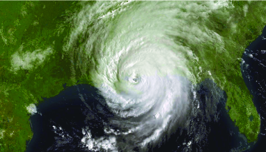
Figure 6: (Color online) The satellite image of Hurricane Katrina 2005 at 14:15, August 29, 2005, Coordinated Universal Time.

To fix the constants $a,\ b$ and $c$ in Eq. (46) for Hurricane Katrina 2005 shown in Fig. 6, we need know the strength (the maximum wind speed), the eye size, and the width of TC Katrina at 14:15, August 29, 2005 UTC. The strength of Katrina can be found in several websites. The data of Table I are downloaded from G .

Table I. Data of Hurricane Katrina downloaded from G .

Time (UTC)	W. Long	N. Lat.	MPH	Time (UTC)	W. Long	N. Lat.	MPH
2005 Aug 23 21:00	75.50	23.20	35	2005 Aug 27 03:00	83.60	24.60	105
2005 Aug 24 00:00	75.80	23.30	35	2005 Aug 27 06:00	84.00	24.40	110
2005 Aug 24 03:00	76.00	23.40	35	2005 Aug 27 09:00	84.40	24.40	115
2005 Aug 24 06:00	76.00	23.60	35	2005 Aug 27 12:00	84.60	24.40	115
2005 Aug 24 09:00	76.40	24.00	35	2005 Aug 27 15:00	85.00	24.50	115
2005 Aug 24 12:00	76.60	24.40	35	2005 Aug 27 18:00	85.40	24.50	115
2005 Aug 24 15:00	76.70	24.70	40	2005 Aug 27 21:00	85.60	24.60	115
2005 Aug 24 18:00	77.00	25.20	45	2005 Aug 28 00:00	85.90	24.80	115
2005 Aug 24 21:00	77.20	25.60	45	2005 Aug 28 03:00	86.20	25.00	115
2005 Aug 25 00:00	77.60	26.00	45	2005 Aug 28 06:00	86.80	25.10	145
2005 Aug 25 03:00	78.00	26.00	50	2005 Aug 28 09:00	87.40	25.40	145
2005 Aug 25 06:00	78.40	26.10	50	2005 Aug 28 12:00	87.70	25.70	160
2005 Aug 25 09:00	78.70	26.20	50	2005 Aug 28 15:00	88.10	26.00	175
2005 Aug 25 12:00	79.00	26.20	50	2005 Aug 28 18:00	88.60	26.50	175
2005 Aug 25 15:00	79.30	26.20	60	2005 Aug 28 21:00	89.00	26.90	165
2005 Aug 25 17:00	79.50	26.20	65	2005 Aug 29 00:00	89.10	27.20	160
2005 Aug 25 19:00	79.60	26.20	70	2005 Aug 29 03:00	89.40	27.60	160
2005 Aug 25 21:00	79.90	26.10	75	2005 Aug 29 05:00	89.50	27.90	160
2005 Aug 25 23:00	80.10	25.90	80	2005 Aug 29 07:00	89.60	28.20	155
2005 Aug 26 01:00	80.40	25.80	80	2005 Aug 29 09:00	89.60	28.80	150
2005 Aug 26 03:00	80.70	25.50	75	2005 Aug 29 11:00	89.60	29.10	145
2005 Aug 26 05:00	81.10	25.40	70	2005 Aug 29 13:00	89.60	29.70	135
2005 Aug 26 07:00	81.30	25.30	70	2005 Aug 29 15:00	89.60	30.20	125
2005 Aug 26 09:00	81.50	25.30	75	2005 Aug 29 17:00	89.60	30.80	105
2005 Aug 26 11:00	81.80	25.30	75	2005 Aug 29 19:00	89.60	31.40	95
2005 Aug 26 13:00	82.00	25.20	75	2005 Aug 29 21:00	89.60	31.90	75
2005 Aug 26 15:00	82.20	25.10	80	2005 Aug 30 00:00	88.90	32.90	65
2005 Aug 26 15:30	82.20	25.10	100	2005 Aug 30 03:00	88.50	33.50	60
2005 Aug 26 18:00	82.60	24.90	100	2005 Aug 30 09:00	88.40	34.70	50
2005 Aug 26 21:00	82.90	24.80	100	2005 Aug 30 15:00	87.50	36.30	35

From Table I, we know that the maximum wind speed of the Katrina 2005 at 14:15, August 29, 2005 UTC is about 130 mph (miles per hour)—i.e.,

$$v_{\max}\sim 130\mbox{\rm\ mph}\sim 200\mbox{\rm\ km \ ph}\sim 2\mbox{\rm\ degree\ ph},\qquad v\equiv\sqrt{\psi_{y}^{2}+\psi_{x}^{2}}.$$ (48)

Comparing Katrina’s satellite image shown in Fig. 6 with the map of New Orleans—say the map shown in Fig. 7 downloaded from track —one can estimate that the eye size ($E$) is about

$$E\sim 1\mbox{\ \rm degree}\sim 100\mbox{\ \rm km}$$

and the width ($W$) of the hurricane is approximately

$$W\approx 10\mbox{\ \rm degree}\approx 1000\mbox{\ \rm km}$$

for Katrina at 14:15, August 29, 2005 UTC. Using these data, we can find that the stream function of Katrina 2005 near the time at 14:15, August 29, 2005 UTC can be approximately described by

$$\psi_{\mbox{Katrina}}\approx y_{0t}x-x_{0t}y-4(2+2\sqrt{r}+r)\exp(-\sqrt{r}),\ \quad(r\equiv(x-x_{0})^{2}+(y-y_{0})^{2}),$$ (49)

which corresponds to the parameter selections

$$a^{2}\sim 8,\ b^{2}\sim 0.5,\ c^{2}\sim 1,$$

in Eq. (46). In the real case, the quantities $a,\ b$ and $c$ should be time dependent. So the description here is only approximate because it is only a solution of the EE instead of the NS equation.

If the strength $v_{\max}$, the size of the hurricane eye $E$, and the width $W$ are assumed to have some errors,

$$v_{\max}\approx 130\pm 10\ \mbox{\rm mph},\ E\approx 1\pm 0.2\mbox{\ \rm degree},\ W\approx 10\pm 2\mbox{\ \rm degree},$$ (50)

then the parameters $a,\ b$ and $c$ in Eq. (46) or (47) have the ranges

$$a^{2}\approx 6.75\sim 9.35,\ b^{2}\approx 0.25\sim 1.25,\ c^{2}\approx 0.9\sim 1.2.$$ (51)

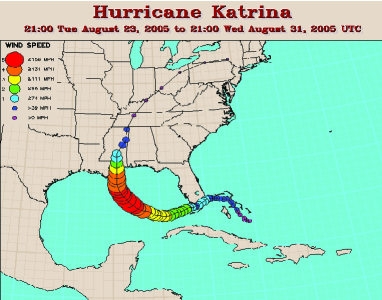
Figure 7: (Color online) The map with the longitude and latitude degree coordinates near the New Orleans and the real track of Hurricane Katrina 2005 from 21:00 Tues., August 23, 2005, to 21:00 Wednes., August 31, 2005 UTC.

In (49), $x_{0}\equiv x_{0}(t)$ and $y_{0}\equiv y_{0}(t)$ can be obtained from the data in Table I. According to Table I, we can find the theoretical fit of hurricane Katrina 2005 from 22:00, August 25, 2005 to 15:00, August 30, 2005 can be approximately described by

$$x_{0}=0.00022t^{2}-0.14t-79,\ y_{0}=0.00073t^{2}-0.07t+26$$ (52)

before 21:00, August 27, 2005 and

$$x_{0}=0.0029t^{2}-0.5t-68,\ y_{0}=0.0023t^{2}-0.2t+29$$ (53)

after 21:00, August 27, 2005. In Eqs. (52) and (53), the units of $x_{0},\ y_{0}$ and $t$ are longitude degree, latitude degree, and hour, respectively, while the initial time $t=0$ is taken as 22:00, August 25, 2005 UTC.

Remark 4. If we fit the track only for the [Longitude, Latitude] positions, we may get a better fit without using any switch point. However, if we fit the track not only for the positions but also for times, we have to select some switch points. Physically speaking, when we use a parabolic line such as (52) to fit the track of a TC, we have to assume that the TC moves under a constant force during the fit time period. The necessary selections of the switch points are caused by the fact that the driven force of the TC is time dependent. Here we find that if we select 21:00, August 27, 2005 as a switch point, then Eqs. (52) and (53) can fit the track quit well (the square error [see later, Eq. (56)] becomes smallest). This means that the TC is approximately driven by two constant forces before and after the turning time, respectively. Actually, approximately speaking, after this switch point, the TC becomes stronger and stronger (see Fig. 7 and/or Table I).

Figure 8 describes the velocity field of Katrina at 14:15, August 29, 2005 UTC ($t=88.15$) when the stream function is given by Eqs. (49) with (53).

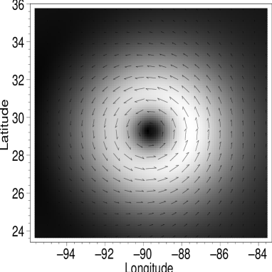
Figure 8: The field and density plot for the velocity field Hurricane Katrina 2005 at 14:15/29/08 described by Eqs. (49) with (53). The strength of the velocity field is expressed by the length of the arrows and the values from left to right at $y=0$ are 0.14, 0.30, 0.53, 0.82, 1.17, 1.55, 1.86, 1.95, 1.60, 0.69, 0.18, 0.89, 1.87, 2.33, 2.31, 2.03, 1.66, 1.30, 0.99, 0.75, and 0.58 (degree per hour), respectively.

In addition, the solution (35)-(36) also provides a relation between the TC track given by $\{x_{0},\ y_{0}\}$ and the strength of the background wind (steering flow).

The stream function of the steering flow, $\psi_{s}$, can be obtained by eliminating the TC term (vortex term) in Eq. (35) with $F_{1}=F_{2}=h_{0}=0$ by setting $F=0$ and then the velocity field flow $\overrightarrow{u}_{s}$ of the background wind reads

$$\overrightarrow{u}_{s}=\{-\psi_{sy},\ \psi_{sx}\}=\{x_{0t},\ y_{0t}\}.$$ (54)

This fact implies that once the background wind, or the large-scale steering flow in the upper air, is known then the motion of the hurricane center can be obtained.

Inversely, if the motion of the hurricane center is known then the steering flow will be obtained at the same time. Therefore, if the position {$x_{0}$, $y_{0}$} of the hurricane center is determined, in a not very long time (say, shorter than one day), one can consider that the velocity of the TC will approximately keep the latest known velocity and then the TC’s new position $\{x_{1}(t_{1}),\ y_{1}(t_{1})\}$ at time $t_{1}$ can be determined by using

$$x_{1}(t_{1})=x_{0}(t_{0})+x_{0t}(t_{0})(t_{1}-t_{0}),\quad y_{1}(t_{1})=y_{0}(t_{0})+y_{0t}(t_{0})(t_{1}-t_{0}).$$ (55)

The concrete steps to predict the track and position of a TC are as follows.

(i) Get the original known position data of a TC from professional meteorologic web site. The concrete position data of a happening TC, say, Katrina, can be read off from some web sites, say, G ; G1 , which are given by some international satellites and updated every six hours and usually three hours (or every hour) close to the landing time.

(ii) Take the coordinate of the fit track. From the web site we can get the position described by longitude and latitude. Because the TCs happen in a quite small area compared to the whole Earth, the fit curve can be taken in a two-dimensional plane. To simplify, the longitude and latitude are defined as $X$ axis $Y$ axes, respectively. The first time recorded on the web site is set as initial time, and the following times are added in order by the time interval.

(iii) Fit the function curve and forecast the track and position. From the first few known positions, it is easy to calculate the fit curve which is the function of time $t$. Usually we can take it possesses the polynomial forms of the time $t$, say, $\{X=x_{0}(t)=\sum_{i=0}^{N}a_{i}t^{i},\ Y=y_{0}(t)=\sum_{i=0}^{N}b_{i}t^{i}\}$. In this paper, we take $N=2$. Finally we should minimize the square error, $\Delta$, among the fit track and the real track

$$\Delta\equiv\sum_{j=n_{1}}^{n_{2}}\left[(x_{0}(t_{j})-x_{j})^{2}+(y_{0}(t_{j})-y_{j})^{2}\right]$$ (56)

by fixing the constants $a_{i}$ and $b_{i}$, where $\{x_{j},\ y_{j}\}$ and $\{x_{0}(t_{j}),\ y_{0}(t_{j})\}$ are the real and fit positions of the hurricane center at time $t_{j}$, $n_{1},\ n_{1}+1,\ ...,\ n_{2}$ are related to the points used to fit the theoretical track $\{x_{0}(t),\ y_{0}(t)\}$, $t=t_{n_{2}}$ corresponds to the time to make the further prediction. Usually, we take $t_{n_{2}}-t_{n_{1}}\sim 24\ ({\mbox{\rm hours}})$ that means the earlier history can be neglected to the hurricane track.

Based on the above descriptions, we can use first few known position data of the hurricane center to predict the possible position of the hurricane some hours later.

Figure 9 displays an example on the TC track [Fig. 9(a)] and the related background wind field [Figs. 9(b)–9(f)]. The zigzag line in Fig. 9(a) is the real track of Katrina 2005 from 21:00/25/08 to 15:00/30/08 (data are read off from G ), and the solid line is our fit (by using all the data in Table I) given by Eqs. (52) and (53). Figures. 9(b)–9(f) reveal the corresponding steering flows at five different times. It is shown that the background wind leads to the change of the direction of the TC track. According to the relation between the track and the steering flow, we can predict the TC track by using several beginning data. The cross points in Fig. 9(a) are our predicted track 6 h before the real one. The same idea has been applied to typhoon Chanchu 2006 JiaLou and Hurricane Andrew 1992 LTJH .

Figure 9: (a). The zigzag line stands for the real TC track of Hurricane Katrina 2005 from 21:00/25/08 to 15:00/30/08 for time and from [79.9,26.2] to [87.5,36.3] for [Longitude, Latitude] position, the smooth line is the fit track by using all the data in Table I and the cross points express our predicted track six hours before the real time. (b)–(f). The corresponding steering flows at 23:00/25/08, 21:00/27/08, 15:00/28/08, 05:00/29/08 and 00:00/30/08 with the strengths 1.33, 1.92, 2.92, 2.67, and 1.08 (degree per hour), respectively.

IV Darboux transformation of the (2+1)-dimensional EE

In Sec. II, we have established a general group theorem (Theorem 2) for the (2+1)-dimensional EE, which can yield various solutions. Furthermore, two solution corollaries on the (2+1)-dimensional EE are obtained by utilizing particular seed solutions.

It is noted that the weak DT theorems given in Li ; LTJH ; LouLi are special cases of the general group Theorem 2. In Li , Li found a (weak) DT of the EE (3) with the Lax pair (6) and (7) for a zero spectral parameter. In LTJH , the weak DT was extended to a general nonzero spectral parameter and many kinds of exact solutions including the solitary, Rossby, conoid, and Bessel waves were obtained subsquently.

Here we derive the weak DT theorem directly from the general group Theorem 2.

Theorem 5 (Weak DT theorem). If $\{\omega^{\prime},\ \psi^{\prime},\ \phi^{\prime}\}$ is a solution of the (2+1)-dimensional EE (3) and its Lax pair (6) and (7) with the spectral parameter $\lambda^{\prime}$, $g(f)$ being an arbitrary function of $f$ which is a given spectral function of (6) and (7) under the spectral parameter $\lambda_{0}$, then

$$\{\omega,\ \psi,\ \phi\}=\{\omega^{\prime}+q,\ \psi^{\prime}+p,\ \exp(g)\phi^{\prime}\}$$ (57)

with the spectral parameter $\lambda$ is a solution of the weak Lax pair (6) and (7) and then Eq. (11) where $p$ and $q$ are determined by

$$q=p_{xx}+p_{yy}$$ (58)

$$[p,\ \ln\phi]=0,$$ (59)

$$[q,\ \ln\phi^{\prime}]+\lambda^{\prime}-\lambda+\lambda_{0}fg_{f}=0.$$ (60)

Proof. Known from the proof of the group Theorem 2, Eqs. (14) and (15) are equivalent to Eqs. (20) and (21). Taking $\xi=x,\ \eta=y$ and $\tau=t$ in Eqs. (20) and (21), we have

$$[\omega,\ \phi^{\prime}]+([\omega,\ g]-\lambda)\phi^{\prime}=0,$$

$$[\psi,\ \phi^{\prime}]+\phi^{\prime}_{t}+(g_{t}+[\psi,\ g])\phi^{\prime}=0.$$

Substituting Eq. (57) into Eq. (20’), we have

$$[\omega^{\prime},\ \phi^{\prime}]+[q,\ \phi^{\prime}]+([\omega^{\prime},\ g]+[q,\ g]-\lambda)\phi^{\prime}$$

$$\quad=\lambda^{\prime}\phi^{\prime}+[q,\ \phi^{\prime}]+g_{f}\lambda_{0}f\phi^{\prime}+([q,\ g]-\lambda)\phi^{\prime}$$

$$\quad=\left\{\lambda^{\prime}-\lambda+\lambda_{0}fg_{f}+[q,\ \ln\phi^{\prime}]\right\}\phi^{\prime}=0.$$

Equation (60) is proven.

Substituting Eq. (57) into Eq. (21’) yields

$$[\psi^{\prime},\ \phi^{\prime}]+[p,\ \phi^{\prime}]+\phi^{\prime}_{t}+(g_{t}+[\psi^{\prime},\ g]+[p,\ g])\phi^{\prime}$$

$$\quad=[p,\ \phi^{\prime}]+[p,\ g]\phi^{\prime}=[p,\ \ln\phi^{\prime}+g]\phi^{\prime}=[p,\ \ln\phi]\phi^{\prime}=0.$$

Equation (59) is proven, and Eq. (58) is a direct result from the definition equation of the vorticity. Theorem 5 is proven. $\Box$

It is interesting that if all the parameters $\lambda,\ \lambda_{0}$ and $\lambda^{\prime}$ are zero and the vorticity of the seed solution is not a constant, the Bäcklund transformation

$$\omega=\omega^{\prime}+q,\ \psi=\psi^{\prime}+p$$

with Eqs. (59) and (60) is equivalent to what were obtained by Li Li . To see it more clearly, one can write Eqs. (59) and (60) in the alternative forms by eliminating $\phi^{\prime}_{y}$ via the Lax pair (6) and (7),

$$\lambda^{\prime}\omega^{\prime}_{x}-[\lambda+\lambda_{0}fg_{f}](\omega^{\prime}+q)_{x}+[\omega^{\prime},\ q][\ln\phi]_{x}=0,$$ (61)

$$[\omega^{\prime}+q,\ p][\ln\phi]_{x}+\lambda^{\prime}p_{x}=0.$$ (62)

The equivalent forms of Eqs. (61) and (62) can also be obtained directly from Eqs. (14) and (15) by setting $\xi=x,\ \eta=y$ and $\tau=t$.

Remark 5. If the seed solution has a constant vorticity, the equation systems (59)–(62) are completely not equivalent. Actually, when one takes a constant vorticity as a seed for the zero spectral parameters, nothing can be obtained from Eqs. (61) and (62). However, one can really find some nontrivial solutions from Eq. (60) with a constant vorticity seed. In LouLi , the weak DT theorem has been used to obtain some types of exact solutions such as the solitary waves, the conoid periodic waves, the Rossby waves, and many kinds of Bessel waves. Here we will not discuss them further.

V Summary and discussion.

The analytical and exact forms of the vortices and circumfluence of the two-dimensional fluid are studied by means of the general symmetry group Theorem 2 of the (2+1)-dimensional EE. Some solution theorems for the (2+1)-dimensional EE are obtained from the group theorem by taking special seed solutions. A special weak DT of the (2+1)-dimensional EE is also obtained from the general group theorem.

The special solution Theorem 4 gives a quite general exact explicit solution which covers many kinds of possible vortices and circumfluence such as the lump-type vortices, dromion-type vortices, ring solitons, etc. The vortex and circumfluence solutions may have applications in various physical fields mentioned in the Introduction and Refs. fluid –H . Particularly, they can qualitatively explain some fundamental problems of TCs such as their eye, track, and the relation between the track and the background wind, and the relation can be used to predict well the TC tracks. Hurricanes and/or typhoons have tremendously and increasingly caused destruction of our world. The method in this paper provides a possible way to understand and study similar disasters intensively. As an original study in this aspect, some introductory analysis by means of our method of Hurricane Katrina 2005 (which almost completely destroyed a whole city, New Orleans) are presented. The technological observations and phenomenological discussions on Hurricane Katrina 2005 can be found in many papers Katrina . In this paper, an approximate analytical expression for the (2+1)-dimensional stream function of Katrina 2005 is obtained. The expression is an exact solution of the (2+1)-dimensional EE and includes some messages including the eye size, the hurricane size, the strength, the relation between the hurricane center and the steering flow, etc. The relation is also used to predict the track of the hurricane.

The discovery of the general group theorem may lead to the discovery of various interesting exact solutions which can be applied to many real physical fields. This paper is just the beginning study in this aspect. There are various important problems should be studied further. For instance, the possible solutions from the general group Theorem 2 are only discussed in three very special cases: (i) the constant vorticity seed (Corollary 1), (ii) the zero spectral parameters without the gauge transformation (Corollary 2, Theorems 3 and 4), and (iii) the pure weak DT case (Theorem 5).

In this paper, we only discuss the (2+1)-dimensional EE. Two types of Lax pairs of the (3+1)-dimensional EE have also been given in Li1 and some special DTs of these Lax pairs have also been given in LTJH . However, these DTs have not yet been utilized to find exact solutions of the (3+1)-dimensional EE. Furthermore, the corresponding symmetry groups similar to that of the (2+1)-dimensional EE given in this paper have not yet been discussed.

The Lax pair and then the DT found in this paper have only weak meaning. Whether the (2+1)-dimensional EE is integrable under some stronger meanings [similar to those of (3+1)-dimensional EE] is still open.

The more general applications of the vortex solutions given in this paper both in atmospheric dynamics and in other physical fields deserve more investigations. Especially, to describe the hurricane more effectively and accurately, some other important factors such as the Coriolis force and the viscosity of the fluid must be considered.

Because of the importance of the EEs and the NS system and their wide applications, the models and all the problems mentioned above are worthy of further study.

- (1) D. Sundkvist, V. Krasnoselskikh, P. K. Shukla, A. Vaivads, M. André, S. Buchert and H. Rème, Nature, 436 825 (2005); G. Pedrizzetti, Phys. Rev. Lett. 94 194502 (2005).
- (2) C. L. Fefferman, http://www.claymath.org /millennium /Navier-Stokes _Equations /Official_Problem_Description. pdf (2000).
- (3) Y. G. Li, J. Math. Phys. 42 3552 (2001).
- (4) Y. G. Li and A. V. Yurov, Stud. Appl. Math. 111 101 (2003).
- (5) S. Y. Lou, X. Y. Tang, M. Jia and F. Huang, Vortices, circumfluence, symmetry groups and Darboux transformations of the Euler equations, nlin.PS/0509039.
- (6) P. H. Chavanis and J. Sommeria, Phys. Rev. Lett. 78 3302 (1997); P. H. Chavanis, ibid 84 5512 (2000).
- (7) E. Cafaro, D. Grasso, F. Pegoraro, F. Porcelli and A. Saluzzi, Phys. Rev. Lett. 80 4430 (1998); D. Del Sarto, F. Califano and F. Pegoraro, ibid 91 235001 (2003).
- (8) V. M. Canuto and M. S. Dubovikov, Ocean Modelling 8 1 (2005).
- (9) C. Girard, R. Benoit, M. Desgagne, Monthly Weather Rev. 133 1463 (2005); S. Kurien, V. S. L’vov, I. Procaccia and K. R. Sreenivasan, Phys. Rev. E 61 407 (2000).
- (10) F. D. M. Haldane and Y. S. Wu, Phys. Rev. Lett. 55 2887 (1985).
- (11) S. Bonazzola, E. Gourgoulhon and J. A. Marck, Phys. Rev. D 56 7740 (1997).
- (12) A. J. Niemi, Phys. Rev. Lett. 94 124502 (2005).
- (13) L.Faddeev, A.J.Niemi, and U.Wiedner, hep-ph/0308240.
- (14) A. J. Leggett, Rev. Mod. Phys. 73 307 (2001).
- (15) I. Chuang, R. Durrer, N. Turok, and B. Yurke, Science 251 1336 (1991); M. J. Bowick, L. Chandler, E.A. Schiff, and A. M. Srivastava, Science 263 943 (1994).
- (16) E. Babaev, A. Sudbø, and N.W. Ashcroft, Nature (London) 431 666 (2004).
- (17) H. Lamb, Hydrodynamics, 6th ed. (Dover, New York, 1945).
- (18) A. A. Abrashkin and E. I. Yakubovich, Sov. Phys. Dokl. 276 370 (1984).
- (19) A. V. Yurov and A. A. Yurova, Theor. Math. Phys., 147 501 (2006).
- (20) S. Y. Lou, M. Jia, F. Huang and X. Y. Tang, Int. J. Theor. Phys. (2007) DOI:10.1007/s10773-006-9327-5.
- (21) F. Huang and S. Y. Lou, Phys. Lett. A 320 428 (2004); V. L. Saveliev, M. A. Gorokhovski, Phys. Rev. E 72 016302 (2005).
- (22) S. Y. Lou and H. C. Ma, Chaos, Solition & Fractals 30 804 (2006).
- (23) S. Y. Lou and H. C. Ma, J. Phys. A: Math. Gen. 38 L129 (2005), S. Y. Lou, Chin. Phys. Lett. 21 1020 (2004).
- (24) S. Y. Lou, J. Math. Phys. 41 6509 (2000).
- (25) X. Y. Tang, S. Y. Lou and Y. Zhang, Phys. Rev. E. 66 046601 (2002).
- (26) K. Emanuel, Nature, 436 686 (2005).
- (27) Q. H. Zhang, S. J. Chen, Y. H. Kuo and R. A. Anthes, Monthly Weather Rev. 133 725 (2005);
- (28) http://www.katrina.noaa.gov/satellite/satellite.html.
- (29) http://fermi.jhuapl.edu/hurr/05/katrina/katrina.txt.
- (30) http://www.ncdc.noaa.gov/img/climate/research/2005/katrina/katrina.gif.
- (31) http://weather.unisys.com/hurricane/atlantic/2005H/KATRINA/track.dat.
- (32) A. Apple, Nature 437 462 (2005); R. Dalton, ibid 300; E. Stokstad, Science 310 1264 (2005); J. Kaiser, ibid 1267 (2005).
- (33) M. Jia, C. Lou and S. Y. Lou, Chin. Phys. Lett. 23 2878 (2006).
- (34) S. Y. Lou and Y. S. Li, Chin. Phys. Lett. 23 2633 (2006).