A Model for Hybrid Simulations of Molecular Dynamics and CFD

Abstract

We propose a method for multi-scale hybrid simulations of molecular dynamics (MD) and computational fluid dynamics (CFD). In the method, usual lattice-mesh based simulations are applied for CFD level, but each lattice is associated with a small MD cell which generates a “local stress” according to a “local flow field” given from CFD instead of using any constitutive functions at CFD level. We carried out the hybrid simulations for some elemental flow problems of simple Lennard-Jones liquids and compared the results with those obtained by usual CFDs with a Newtonian constitutive relation in order to examine the validity of our hybrid simulation method. It is demonstrated that our hybrid simulations successfully reproduced the correct flow behavior obtained from usual CFDs as far as the mesh size $\Delta x$ and the time-step $\Delta t$ of CFD are not too large comparing to the system size $l_{\rm MD}$ and the sampling duration $t_{\rm MD}$ of MD simulations performed at each time step of CFDs. Otherwise, simulations are affected by large fluctuations due to poor statistical averages taken in the MD part. Properties of the fluctuations are analyzed in detail.

I Introduction

Hydrodynamics of complex fluids are of particular importance in various science and engineering fields, such as fluid mechanics, soft matter science, mechanical engineering, chemical engineering, and so on. Because of the complicated couplings between internal degree of freedoms of complex fluids and their flow behavior, conventional treatments, based on usual assumptions such as non-slip boundary conditions and linear Newtonian constitutive relations, are often invalid. Striking examples can be seen in systems such as colloidal dispersions, polymeric liquids, granular matters, and liquid crystals. Those systems are known to exhibit peculiar flow behaviors, e.g., shear thinning or thickening, viscoelasticity, jamming, flow induced phase transition, etc.

Although there exits huge accumulation of experimental and theoretical studies on the rheology of complex fluids, performing computational fluid dynamics (CFD) simulations are not yet common for complex fluids since reliable constitutive equations are often unknown for those systems. On the other hand, there exists a different problem also for microscopic approaches such as molecular dynamics (MD) simulations, while constitutive equations are no more necessary in this case. The characteristic time and length scales of complex fluids easily become several orders larger than those of microscopic scales. Therefore, most hydrodynamic problems of complex fluids are yet out of reach of microscopic MD simulations. To overcome those serious limitations mentioned above, we aim to develop a new multi-scale method which is for performing hybrid simulations of MD and CFD valid for complex fluids without any constitutive equations.

Various methods for hybrid simulations of MD and CFD has already been proposed by several researchers. Most of those methods are based on “domain decomposition” for which MD simulations are applied only around the points of interest, i.e., in the vicinity of defects, boundaries, interfaces, where details of molecular motions are important, while the remaining regions are treated only by CFD. art:95OT ; art:00FWF ; art:03DC ; art:05DFC ; art:04NCER ; art:04NCR ; art:06NRC ; art:07LCNR ; art:07R ; art:07YST Exchange of information between MD and CFD is performed in a coupling regions where each system is subjected to some constrains to take the consistency of the two systems. This kind of hybrid method is expected to be useful specially for problems including interfaces, such as adhesion, friction, anchoring of crystal liquids, stick-slip motions, etc.

In order to apply hybrid methods of MD and CFD to hydrodynamics of complex fluids, a different type of approach is probably needed. Our strategy for this is straightforward. We try to develop a multi-scale hybrid method based on the local equilibrium assumption. Here CFD is used as a fluid solver, while MD simulations are used only to generate local properties, such as constitutive relations of the fluid under consideration, by performing local statistical sampling in a consistent matter. The numerical algorithm is rather simple. We perform usual lattice-mesh based CFD simulations at an upper level, but each mesh-node is associated with a small lower level MD cell which passes a “local stress” to CFD according to a “local flow field” given from CFD to MD instead of using any constitutive functions at CFD level. MD simulations thus have to be performed at all node points and at every time steps of CFD.

One might think that the simulations would be be much faster if we construct tabular database of the constitutive relations by performing MD simulations in advance under many different simulation parameters and refer the table from CFD. The “tabular approach” works much effective for simple fluids for which the constitutive relations depend only on a few parameters, such as the density, temperature, and shear rate. In the case of complex fluids, however, the number of parameters to be considered can be huge depending on the local quantities to be considered. In the case of charged systems for example, the local stress depends also on the local compositions and chemical potentials of ions and the local electric field, etc. Although we used only simple Lennard-Jones liquid in the present study, we adopt the local sampling strategy rather than the tabular contraction strategy to be more general. The main purpose of the present study is to examine the validity of our multi-scale hybrid model by performing some simple demonstrations of the method. Efficiency and drawback of both strategies will be considered in future for more specific problems. An idea similar in spirit to the present method was also put forward earlier by W. Ren and W. E. art:05RE

The hybrid simulation method is described in Sec. II, and some demonstrative results for one- and two-dimensional flows of simple Lennard-Jones liquids are shown in Sec. III. A special attention is put on the efficiency and the reliability of our hybrid method there. The simulation results obtained by our multi-scale hybrid method are compared with those of normal CFDs with a Newtonian constitutive relation. The validity of our method is discussed in Sec. IV, and a summary is given in Sec. V.

II Hybrid Model

Incompressible flows for isotropic materials are described by the following equations,

$$\frac{\partial v_{\alpha}}{\partial x_{\alpha}}=0,$$ (1)

$$\frac{\partial v_{\alpha}}{\partial t}+v_{\beta}\frac{\partial v_{\alpha}}{\partial x_{\beta}}=\frac{1}{\rho}\frac{\partial P_{\alpha\beta}}{\partial x_{\beta}}+g_{\alpha},$$ (2)

where $x_{\alpha}$ is the Cartesian coordinate system, $t$ the time, $v_{\alpha}$ the velocity, $\rho$ the density, $P_{\alpha\beta}$ the stress tensor, and $g_{\alpha}$ the external force per unit mass. Here and after the subscripts $\alpha$, $\beta$, and $\gamma$ represent the index in Cartesian coordinates, i.e. {$\alpha$, $\beta$, $\gamma$} = {$x$, $y$, $z$}, and the summation convention is used. The stress tensor $P_{\alpha\beta}$ is written in the form,

$$P_{\alpha\beta}=-p\delta_{\alpha\beta}+T_{\alpha\beta},$$ (3)

where $p$ is the pressure and $\delta_{\alpha\beta}$ is the Kronecker delta. Here we assumed that the diagonal component of the stress tensor is isotropic. The off-diagonal stress tensor is symmetric $T_{\alpha\beta}=T_{\beta\alpha}$ and traceless $T_{\alpha\alpha}$=0. art:45R In order to solve the above equations, one needs a constitutive relation for the stress tensor $T_{\alpha\beta}$. In our hybrid method, instead of using any explicit formulas such as the Newtonian constitutive relation, $T_{\alpha\beta}$ is computed directly by MD simulations.

II.1 CFD Scheme

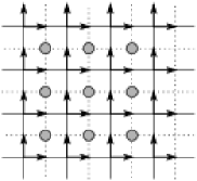
We use a lattice-mesh based finite volume method with a staggered arrangement for vector and scalar quantity.book:02FP See Fig. 1. The control volume for a vector quantity is a unit square surrounded by dashed lines and that for a scalar quantity is a unit square surrounded by solid lines. Eqs (1) and (2) are discretized by integrating the quantities on each control volume. As for numerical time integrations, we use the fourth order Runge-Kutta method, where a single physical time step $\Delta t$ is divided into four sub-steps. More concretely, the time evolution of a quantity $\phi$, which is to be determined by the equation $\partial\phi/\partial t$=$f(t,\phi)$, is written as

$$\phi_{n+\frac{1}{2}}^{*} =\phi^{n}+\frac{\Delta t}{2}f(t_{n},\phi^{n}),$$ (4a)

$$\phi_{n+\frac{1}{2}}^{**} =\phi^{n}+\frac{\Delta t}{2}f(t_{n+\frac{1}{2}},\phi^{*}_{n+\frac{1}{2}}),$$ (4b)

$$\phi_{n+1}^{*} =\phi^{n}+\Delta tf(t_{n+\frac{1}{2}},\phi^{**}_{n+\frac{1}{2}}),$$ (4c)

$$\phi^{n+1} =\phi^{n}+\frac{\Delta t}{6}\left[f(t_{n},\phi^{n})+2f(t_{n+\frac{1}{2}},\phi^{*}_{n+\frac{1}{2}})+\right.$$

$$\hskip 56.9055pt\left.2f(t_{n+1/2},\phi^{**}_{n+1/2})+f(t_{n+1},\phi^{*}_{n+1})\right].$$ (4d)

Time evolution of the fluid velocity $\bm{v}$ is computed by the above set of equations. On the other hand, the pressure $p$ is determined so that the fluid velocity satisfies the incompressible condition (1) at each sub-step. The procedure at each sub-step is written as

$$p=\tilde{p}+\psi,$$ (5a)

$$\bm{v}=\tilde{\bm{v}}-\tau\nabla\psi,$$ (5b)

$$\triangle\psi=\frac{1}{\tau}\nabla{\tilde{\bm{v}}},$$ (5c)

where $\tilde{p}$ is the pressure obtained at the previous sub-step, $\tilde{\bm{v}}$ is the velocity obtained by solving equation (4) at the present sub-step, and $\tau$ is the time increment of the sub-step. The remaining three components of the tensor $T_{\alpha\beta}$ are to be computed directly by MD simulations. The detail of the method is described in the next subsection. Note that the calculations of $T_{\alpha\beta}$ is carried out at each sub-step of equation (4).

Figure 1: Staggered arrangement of vector quantity, the velocity $\bm{v}$, and scalar quantity, the pressure $p$ and density $\rho$, on a lattice-mesh grid.

Figure 2: Schematic diagram for the hybrid scheme. (a) CFD simulations are performed in a reference coordinate ($x$,$y$,$z$), while MD simulations are performed in a rotated coordinate ($x^{\prime}$,$y^{\prime}$,$z^{\prime}$) so that the diagonal components of $E^{\prime}_{\alpha\beta}$ become all zero with the procedure described in Sec II B. The CFD system is discretized into cubic subsystems whose side length is $\Delta x$. Each subsystem is associate with a MD cell, whose side length is $l_{\rm MD}$, with Lees-Edward periodic boundary condition under shear deformation. (b) A schematic time evolution of our multi-scale method. CFD simulation proceeds with a time step of $\Delta t$, MD simulation is carried out for a lapse of time $t_{\rm MD}$ only to sample local stress $T^{\prime}_{\alpha\beta}$ at each node point and time step of CFD.

II.2 Computation of Local Stress by MD

We compute the local stresses by MD simulations according to the local strain rates, rather than the local flow velocities themselves, computed at the CFD level. A schematic diagram of the method is depicted in Fig. 2. At the CFD level, the local strain rate tensor $E_{\alpha\beta}$ is defined as

$$E_{\alpha\beta}=\frac{1}{2}\left(\frac{\partial v_{\alpha}}{\partial x_{\beta}}+\frac{\partial v_{\beta}}{\partial x_{\alpha}}\right),$$ (6)

where the incompressible condition, $E_{\alpha\alpha}$=0, is to be satisfied. We can now define a rotation matrix $\Theta$ with which the strain rate tensor $E_{\alpha\beta}$ is transformed to

$$E^{\prime}=\Theta E\Theta^{\rm T}=\left(\begin{array}[]{ccc}0&E^{\prime}_{xy}&E^{\prime}_{xz}\\ E^{\prime}_{yx}&0&E^{\prime}_{yz}\\ E^{\prime}_{zx}&E^{\prime}_{zy}&0\end{array}\right),$$ (7)

where the diagonal components all vanish. This transformation makes performing MD simulations much easier with the usual Lees-Edwards periodic boundary condition for simple shear flows under the assumption that each off-diagonal the component of the local stress tensors depends only on the corresponding component of the local strain rate tensors, respectively. The off-diagonal stress tensor $T^{\prime}_{\alpha\beta}$ is computed according to $E^{\prime}_{\alpha\beta}$ and then pass to CFD after transforming back to the original coordinates, $T_{\alpha\beta}$. For one- or two-dimensional flows [$\partial/\partial z$=0 and $v_{z}$=0], $\Theta$ and $E^{\prime}$ are expressed as

$$\Theta =\left(\begin{array}[]{cc}\cos\theta&\sin\theta\\ -\sin\theta&\cos\theta\end{array}\right),$$ (10)

$$E^{\prime}_{xy}=E^{\prime}_{yx} =-E_{xx}\sin 2\theta+E_{xy}\cos 2\theta,$$ (11)

where

$$\theta=\frac{1}{2}\tan^{-1}\left(-\frac{E_{xy}}{E_{xx}}\right).$$ (12)

Non-equilibrium MD simulations for simple shear flows in the rotated Cartesian coordinates are performed in many MD cells according to the local strain rate $E^{\prime}$’s defined at each lattice node of the CFD. The number of particles in each MD cell is 256 if not mentioned. Once a local stress tensor $P^{\prime}_{\alpha\beta}$ is obtained at the MD level, the local stress at each lattice node $P_{\alpha\beta}$ in the original coordinate system is obtained by combining the pressure $p$ obtained a priori by CFD and a tensor $T^{\prime}_{\alpha\beta}$ obtained by subtracting the isotropic normal stress components from $P^{\prime}_{\alpha\beta}$ as

$$P=\Theta^{T}[-p{\rm I}+T^{\prime}]\Theta=-p{\rm I}+\Theta^{T}T^{\prime}\Theta,$$ (13)

where I is the unit tensor. For one- or two dimensional flows, we can use $T^{\prime}_{xx}$=$T^{\prime}_{yy}$=0 and $T^{\prime}_{xy}$=$T^{\prime}_{yx}$=$P^{\prime}_{xy}$.

In the non-equilibrium MD simulations, we use the Lees-Edwards sheared periodic boundary condition to a cubic MD. The temperature is kept at a constant by using a thermostat.art:84BC ; book:89AT The stress $P^{\prime}_{\alpha\beta}$ is averaged in steady states after transient behavior vanished.

III Numerical Computation

We have carried out the hybrid simulations for one- and two-dimensional flows of a simple liquid composed of the Lennard-Jones (LJ) particles interacting via the potential

$$v^{\rm LJ}(r)=4\varepsilon\left[\left(\frac{\sigma}{r}\right)^{12}-\left(\frac{\sigma}{r}\right)^{6}\right].$$ (14)

In the present simulations, the potential is truncated at $r$=$r_{\rm c}$ and sifted to zero at the distance for computational efficiency. We considered only the cases where the temperature $T$ and the fluid density $\rho$ are uniform and constant over the CFD systems and the external force is neglected, $g_{\alpha}$=0. The reduced temperature $T^{*}$=$Tk/\varepsilon$ and reduced density $\rho^{*}$=$\rho\sigma^{3}/m$, where $k$ is the Boltzmann constant and $m$ is the mass of a single LJ particle, are fixed at $T^{*}$=1.0 and $\rho^{*}$=0.8 in the simulations. Here and after, non-dimensional quantities normalized by the energy and length parameters of the Lennard-Jones potential, $\varepsilon$ and $\sigma$, are denoted by the superscript “$\ast$”.

In the following, $\Delta t$ and $\Delta x$ represent the time-step and the mesh size of CFD calculations, and $t_{\rm MD}$ and $l_{\rm MD}$ represent the sampling time and the side length of a MD cell, respectively. The two parameters $\Delta t/t_{\rm MD}$ and $\Delta x/l_{\rm MD}$ represent the efficiency of our hybrid simulations. We have carried out hybrid simulations with several different values of the parameters and compared the results with those obtained by usual CFDs. In the present simulations we fixed $t^{*}_{\rm MD}$=0.005 and $l^{*}_{\rm MD}$=6.84, while $\Delta t$ and $\Delta x$ are changed as listed in Table 1.

III.1 Pressure-driven channel flows

The Lennard-Jones liquid with $r^{*}_{c}$=2.5 is contained in channel composed of two parallel plates located at $x_{1}$=$\pm L/2$ and subjected to a pressure gradient in $y$-direction. We performed one- and two-dimensional simulations for this pressure-driven channel flows. The pressure gradient is set as $\Delta p/(\rho U^{2}/L)$=1.25, where $\Delta p$ is the pressure difference over a distance $L$, and $U$ is a characteristic flow velocity. Non-slip boundary condition is applied on the two plates.

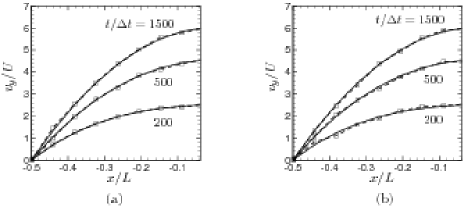
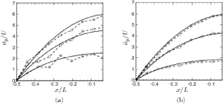
The results of one-dimensional simulations are shown in Figs. 3 and 4. A symmetric condition is used at $x$=0, and the computational domain [$-L/2$,0] is divided into eight slits. Parameters used in the simulations are listed as SP I–III in Table 1. In the corresponding CFD simulation, viscosity is set as $\eta^{*}$=2.0, which is for the LJ liquid with $r^{*}_{c}=2.5$ at $T^{*}$=1.0 and $\rho^{*}$=0.8. The Reynold number defined as $\rho UL/\eta$ is fixed at 40. It is clearly shown in Fig. 3 that the results obtained by the present hybrid simulations well agree with those of usual CFDs for the case $\Delta t/t_{\rm MD}<$ 2 and $\Delta x/l_{\rm MD}<$ 2. When the parameters become large, instantaneous velocity profiles tend to fluctuate as seen in Fig. 4. It should be noted that the fluctuations can be removed almost perfectly by taking time averages. This means that the mean values of the fluctuation is almost zero, i.e., the fluctuation might be removed also by applying some filtering, etc. We will discuss on this point later.

Figure 3: The velocity profiles obtained by one dimensional computations for the pressure-driven channel flow. Simulation Parameters are summarized as SP I in Table 1 for (a) and SP II in Table 1 for (b). The solid lines show the results of usual CFD simulation, and dotted lines and square symbols show the results of the present hybrid simulation.

Figure 4: The velocity profiles obtained by one dimensional computations for the pressure-driven channel flow. Simulation parameters are summarized as SP III in Table 1. Time evolutions of the velocity profile after an application of pressure gradient in y-direction at $t$=0. Instantaneous profiles at $t/\Delta t=200$, $500$, and $1500$ are shown in (a), while the velocity profiles are time averaged over $t/\Delta t=[0,300]$, $[300,600]$, and $[1200,1500]$ in (b). The squares show results of the hybrid simulations, and the dotted lines present the corresponding CFD results for comparison.

The results of two-dimensional simulations are shown in Fig. 5. The computational domain is now [-$L/2$,$L/2$]$\times$[0,$L/2$] and divided into 16$\times$8 uniform lattices. Non-slip boundary condition is used at $x$=$\pm L/2$. At $y$=0 and $L/2$, periodic condition is used for the velocity, and the pressure is set as $p(x,L/2)$=$p(x,0)-0.5\Delta p$. Here we assumed Stokes flow, i.e., the second term of the left-hand-side of Equation (2) is dropped in the computation. It is seen that, at each time step, the velocity fluctuations are much smaller than the pressure fluctuations. This is clearly due to the incompressible condition to be imposed to the velocity. The velocity also fluctuates immediately after solving Eq. (2), however the incompressible condition Eq. (1) tends to adjust it. The pressure fluctuations can be removed also by taking time averages.

Figure 5: The steady-state flow profiles of the pressure-driven channel flow obtained by a two-dimensional calculation. Simulation parameters are summarized as SP IV in Table 1.

III.2 Two-dimensional cavity flows

Lennard-Jones liquid with $r^{*}_{c}=2^{1/6}$ is contained in a square box whose side length is $L$. At $t$=0, the upper wall starts to move from left to right at a velocity $v_{w}$=$U$. Non-slip boundary condition is applied at each wall; $v_{x}$=$U$ and $v_{y}$=0 at $y$=$L$, and $v_{x}$=$v_{y}$=0 at other walls. At left- and right- upper corners, $v_{x}$=$U$ and $v_{y}$=0 is applied. The results of the hybrid simulations are shown in Figs. 6 and 7. The computational domain is divided into 32$\times$32 uniform lattices. Values of parameters used in the present simulations are listed as SP V-VII in Table 1. The Reynolds number is defined as $\rho UL/\eta$, and the viscosity of the corresponding LJ fluid is $\eta^{*}$=1.7.

Fig. 6 shows the steady-state velocity profiles time-averaged over $t/\Delta t$=[950,1000]. It is clear that our hybrid method can successfully reproduce the characteristic flow properties of cavity flows with different Reynolds numbers.

Figure 6: The steady-state velocity profile for the cavity flow. Simulation parameters are summarized as SP V in Table 1 for (a), SP VI for (b), and SP VII for (c). The velocity profiles are time averaged over $t/\Delta t$=[950,1000]

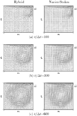
Fig. 7 shows time evolutions of velocity profiles for the case of Re=980 after a sudden application of upper-wall sliding at $t=0$. Here, the results obtained by hybrid simulations are compared with those of usual CFD simulations. It is seen commonly that a small vortex first appears at the upper-right corner is moving gradually toward the center of the box with increasing the size of the vortex as time passes. The agreements between hybrid simulations and CFDs are very well. Our hybrid method is confirmed to reproduce successfully the time-evolution while large fluctuations are seen in the instantaneous velocity profiles.

Figure 7: Time evolutions of the velocity profile for the cavity flow with Re=980. The left column shows the Hybrid simulations and the right column shows the corresponding CFD results. Simulation parameters are summarized as SP VII in Table 1.

1d channel flow
		$l^{*}_{\rm MD}$		$t^{*}_{\rm MD}$		$L^{*}$		$U^{*}$		$\Delta x/l_{\rm MD}$		$\Delta t/t_{\rm MD}$
SP I		6.84		1.87		116.3		0.86		1.0		1.0
SP II		6.84		3.74		232.6		0.43		2.0		2.0
SP III		6.84		7.49		465.1		0.22		4.0		4.0
2d channel flow
		$l^{*}_{\rm MD}$		$t^{*}_{\rm MD}$		$L^{*}$		$U^{*}$		$\Delta x/l_{\rm MD}$		$\Delta t/t_{\rm MD}$
SP IV		6.84		3.74		232.6		0.43		2.0		2.0
2d cavity flow
		$l^{*}_{\rm MD}$		$t^{*}_{\rm MD}$		$L^{*}$		$U^{*}$		$\Delta x/l_{\rm MD}$		$\Delta t/t_{\rm MD}$
SP V		6.84		4.68		218.9		0.46		1.0		1.0
SP VI		6.84		9.36		437.8		0.91		2.0		2.0
SP VII		6.84		3.11		875.5		1.83		4.0		4.0

Table 1: Simulation parameters.

IV Discussion

As mentioned above, the ratios $\Delta t/t_{\rm MD}$ and $\Delta x/l_{\rm MD}$ measure the efficiency of our hybrid simulations. Larger the ratios, simulations are more efficient, however, the statistical fluctuations also become large. For example, in a case of $\Delta t/t_{\rm MD}$=$\Delta x/l_{\rm MD}$=4, computational efficiency is, roughly speaking, $4^{D}\times 4$ times more efficient than a full MD simulation of a $D$-dimensional cubic system. As we have already seen in one- and two-dimension cases, numerical results of our hybrid simulations show good agreements with those of CFD simulations as far as $\Delta t/t_{\rm MD}$ and $\Delta x/l_{\rm MD}$ remain small, say $\Delta t/t_{\rm MD}<2$ and $\Delta x/l_{\rm MD}<2$. In fact, the normalized standard deviation, $\int_{L}dx\int_{T}dt(v-v_{\rm NS})^{2}/TL$, of the velocity profiles of hybrid method, $v$, and those of CFDs, $v_{\rm NS}$, are less than 0.02 and 0.07 for the cases of Fig. 3 (a) and for Fig. 3 (b). As the ratios increase, solutions of our hybrid model start to fluctuate around the corresponding CFD results. The deviation becomes about 0.6 in the case of Fig. 4 (a). It is worth mentioning that the instantaneous velocity fluctuations are notable at each time step, however, they can be removed almost perfectly by taking time averages. In the following part, we will discuss the nature of the fluctuations more in detail to examine possibilities of effectively controlling them in our future simulations where correct thermal fluctuations will be included.

To handle the statistical noise explicitly, we rewrite Eq. (13) as

$$P=-pI+\Theta^{T}(T_{*}^{\prime}+R^{\prime})\Theta,$$ (15)

where the off-diagonal stress tensor $T^{\prime}$, which is to be determined by MD sampling, is decomposed into the non-fluctuating stress $T^{\prime}_{*}$ and the fluctuating random stress $R^{\prime}$ due to the thermal noise. The magnitude of each component of the random stress included in MD sampling $\langle R_{{\rm MD}pq}^{\prime 2}\rangle$, where $p$ and $q$ represent the index in Cartesian coordinates and do not follow the summation convention, should depend both on the size of the MD cell $l_{\rm MD}$ and the length of time $t_{\rm MD}$ over which average is taken at the MD level; $\langle R_{{\rm MD}pq}^{\prime 2}\rangle$=$\langle\bar{R}_{pq}(l_{\rm MD},t_{\rm MD})^{2}\rangle$, where $\bar{R}(l,t)$ represents the random stress tensor averaged in a cubic with a side length $l$ and over a time duration $t$.

At the CFD level which is discretized with a mesh size $\Delta x$ and a time-step $\Delta t$, the physically correct magnitude should be $\langle R_{{\rm CFD}{pq}}^{\prime 2}\rangle$ =$\langle\bar{R}_{pq}(\Delta x,\Delta t)^{2}\rangle$. If the central limit theorem, $\langle\bar{R}_{pq}(l,t)^{2}\rangle$$\propto 1/l^{D}t$ is assumed, the following simple formula can be used.

$$\langle R_{{\rm MD}{pq}}^{\prime 2}\rangle=\left(\frac{\Delta x}{l_{\rm MD}}\right)^{D}\left(\frac{\Delta t}{t_{\rm MD}}\right)\langle R_{{\rm CFD}{pq}}^{\prime 2}\rangle.$$ (16)

This finally leads to the following very useful expression for the correctly fluctuating stress tensor $P$,

$$P=-pI+\Theta^{T}\left[T^{\prime}_{*}+\sqrt{\left(\frac{l_{\rm MD}}{\Delta x}\right)^{D}\left(\frac{t_{\rm MD}}{\Delta t}\right)}R^{\prime}_{\rm MD}\right]\Theta$$ (17)

to be used in CFD instead of Eq. (13). This equation indicates that if we can re-weight randomly fluctuating part ${R}^{\prime}$ while the non-fluctuating part $T^{\prime}_{*}$ being untouched, hydrodynamic simulations including correct thermal fluctuations can be done for complex fluids within the present framework.

We note that the important key toward the development of fluctuating hybrid simulation is the separation of $T^{\prime}_{*}$ and ${R}^{\prime}$. We thus carried out spectral analysis for the fluctuations in the total stress tensor computed directly from MD simulations $T^{\prime}=T^{\prime}_{*}+{R}^{\prime}$. The discrete Fourier transformation of $T^{\prime}_{xy}$ is defined as

$$\varPi^{\prime}_{xy}\{\bm{k}\}=\frac{1}{4M^{2}}\sum_{n_{x}=0}^{2M-1}\sum_{n_{y}=0}^{2M-1}\hat{T}^{\prime}_{xy}\{\bm{x}\}\exp(-i{\bm{k}}\cdot{\bm{x}}),$$ (18)

where ${\bm{x}}=(n_{x}\Delta x,n_{y}\Delta x)$ is the position of each lattice node $(n_{x},n_{y})$, ${\bm{k}}=(2\pi m_{x}/L,2\pi m_{y}/L)$ is the wave vector, $n_{x},n_{y},m_{z},m_{y}$ are integers, M is the lattice number in each $x$- and $y$-axis, and $\hat{T}^{\prime}_{xy}\{{\bm{x}}\}$ is defined as $\hat{T}^{\prime}_{xy}\{{\bm{x}}\}$=$T^{\prime}_{xy}(x+\Delta x/2,y+\Delta x/2)$ for $0\leq x,y\leq L$, $\hat{T}^{\prime}_{xy}\{{\bm{x}}\}$=$T^{\prime}_{xy}\{2L-x,y\}$ for $L<x\leq 2L$, and $\hat{T}^{\prime}_{xy}\{{\bm{x}}\}$=$T^{\prime}_{xy}\{x,2L-y\}$ for $L<y\leq 2L$.

Figure 8: The fluctuations of $T^{\prime}_{xy}$ for the case of cavity flow with Re=59. The power spectra $\langle|\varPi^{\prime}_{xy}\{\bm{k}\}|^{2}\rangle$ for the present multi-scale model with $\Delta x/l_{\rm MD}=\Delta t/t_{\rm MD}=1$ is shown in (a) and the corresponding result from the fluctuating hydrodynamics is shown in (b) for a comparison. $\varPi^{\prime}_{xy}$ represents the discrete Fourier transform of $T^{\prime}_{xy}$. $m_{\alpha}$ is defined as $m_{\alpha}$=$(L/2\pi)k_{\alpha}$, where ${\bm{k}}$ is the wave vector. The insets on each figure shows the $\langle|\varPi^{\prime}_{xy}|^{2}\rangle$-$m_{x}$ plane.

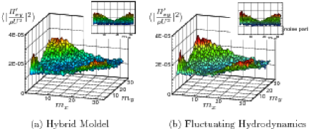
The power spectra $\langle|\varPi^{\prime}_{xy}\{\bm{k}\}|^{2}\rangle$ calculated from our hybrid simulations of driven cavity flows are plotted in Fig. 8 (a) for the case of $\Delta t/t_{\rm MD}=\Delta x/l_{\rm MD}=1$. This corresponds to the case of Fig. 6 (a). The angle bracket $\langle\cdots\rangle$ means the time average taken in the steady state at CFD level. One can see that the overall structure is rather simple. There exists a relatively large peak around ${\bm{k}}=0$ and rather flat distributions throughout the ${\bm{k}}$ plane. The former corresponds to the contributions from the non-fluctuating part $T^{\prime}_{*}$ and the later corresponds to the contributions from the random stress $R^{\prime}$. The same quantity obtained by conventional fluctuating hydrodynamics using a constant Newtonian viscosity and the random stress whose intensity is determined by the fluctuation-dissipation theorembook:59LL is shown in Fig. 8 (b) for a comparison.note1 Those two plots are surprisingly similar to each other including the fluctuation part. This means that our hybrid simulation generates fluctuations quite consistent with the fluctuating hydrodynamics with fluctuation-dissipation theorem in the case of $\Delta x/l_{\rm MD}$=$\Delta t/t_{\rm MD}$=1.

Next, one see how the fluctuations depend on the ratios $\Delta x/l_{\rm MD}$ and $\Delta t/t_{\rm MD}$ in Fig. 9. Here, comparing to the reference case (a) [$\Delta x/l_{\rm MD}$=$\Delta t/t_{\rm MD}$=2], the number of particles used in MD simulations are doubled in the case of (b) [$\Delta x/l_{\rm MD}$=1.59, $\Delta t/t_{\rm MD}$=2], and both the number of particles and the sampling duration to take time average are doubled in the case of (c) [$\Delta x/l_{\rm MD}$=1.59, $\Delta t/t_{\rm MD}$=1]. It is seen that the noise intensity decreases with decreasing ratios $\Delta x/l_{\rm MD}$ and $\Delta t/t_{\rm MD}$ in a consistent way to the central limiting theorem Eq. (16) i.e., the noise intensity in (b) is about a half of that in (a), and the intensity in (c) is about one fourth of that in (a).

Figure 9: The fluctuations of $T^{\prime}_{xy}$ for the case of cavity flow with Re=235. The power spectra $\langle|\varPi^{\prime}_{xy}\{\bm{k}\}|^{2}\rangle$ is plotted in (a) for the case of Fig. 6 (b). Only the number of particles are doubled in (b), while other parameters are unchanged from (a). In (c), both the number of particles and the sampling time of $T^{\prime}_{xy}$ are doubled. $\varPi^{\prime}_{xy}$ represents the discrete Fourier transform of $T^{\prime}_{xy}$. $m_{\alpha}$ is defined as $m_{\alpha}$=$(L/2\pi)k_{\alpha}$, where ${\bm{k}}$ is the wave vector. The insets on each figure shows the $\langle|\varPi^{\prime}_{xy}|^{2}\rangle$-$m_{x}$ plane.

Finally, we mention other recently proposed methods based on a similar idea. In the reference art:05RE, , a hybrid method is proposed for bulk and boundary problems. Several problems for one- or two-dimensional flows of simple Lennard-Jones and dumb-bell liquids are considered. We note that the present multi-scale hybrid method is different from the methods proposed in those references particularly on the constructions of the stress tensor. In our method, a rotation matrix which effectively transforms the tensors in the Cartesian coordinates used in CFD and MD simulations. We also replace the isotropic part of the stress tensor calculated by MD simulations with the pressure imposed by the incompressible condition in CFD. More specifically, only the pure shear stress is passed from MD to CFD for numerical efficiency and consistency.

V Summary

We proposed a multi-scale method for hybrid simulations of MD and CFD. Our method is based on direct computations of the local stress by performing non-equilibrium MD simulations according to the local flow field at all lattice nodes of CFD. The validity of the method is tested by comparing the numerical results obtained by our method and usual CFD. We found that the results obtained by our hybrid method agree well with those of usual CFDs with the Newtonian constitutive relation when the mesh size and the time-step of CFD are not too large comparing to the cell size and sampling time of MD simulations. When the ratios $\Delta t/t_{\rm MD}$ and $\Delta x/l_{\rm MD}$ become large, there appear large fluctuations in flow field of our hybrid simulations. It was, however, clarified by the spectral analysis that the stress tensor $T^{\prime}$ computed by MD simulations has a very simple structure. It is composed of the non-fluctuating component $T^{\prime}_{*}$ and the random component ${R^{\prime}}$ which seem to obey simple central limiting theorem according to the system size and the duration of the MD sampling. We confirmed that the power spectrum of the non-fluctuating component $T_{*}^{\prime}$ in MD sampling agrees well with that computed in usual CFD without fluctuation. The power spectrum of ${R^{\prime}}$ also showed a good agreement with numerical results of the fluctuating hydrodynamics which obeys the fluctuation-dissipation theorem.

References

- (1) S. T. O’Connell and P. A. Thompson, “Molecular dynamics–continuum hybrid computations: A tool for studying complex fluid flows,” Phys. Rev. E 52, R5792 (1995).
- (2) E. G. Flekkoy, G. Wagner, and J. Feder, “Hybrid model for combined particle and continuum dynamics,” Europhys. Lett. 52, 271 (2000).
- (3) R. Delgado-Buscalioni and P. V. Conveney, “Continuum-particle hybrid coupling for mass, momentum, and energy transfers in unsteady fluid flow,” Phys. Rev. E 67, 046704 (2003).
- (4) R. Delgado-Buscalioni, E. G. Flekkoy, and P.V. Coveney, “Fluctuations and continuity in particle-continuum hybrid simulations of unsteady flows based on flux-exchange,” Europhys. Lett. 69, 959 (2005).
- (5) X. Nie, S. Chen, W. E, and M. O. Robbins, “A continuum and molecular dynamics hybrid method for micro- and nano-fluid flow,” J. Fluid Mech. 500, 55 (2004).
- (6) X. Nie, S. Chen, and M. O. Robbins, “Hybrid continuum-atomistic simulation of singular corner flow,” Phys. Fluids 16, 3579 (2004).
- (7) X. Nie, M. O. Robbins, and S. Chen, “Resolving Singular Forces in Cavity Flow: Multiscale Modeling from Atomic to Millimeter Scales,” Phys. Rev. Lett. 96, 134501 (2006).
- (8) J. Liu, S. Chen, X. Nie, and M. O. Robinns, “A continuum-atomistic simulation of heat transfer in micro- and nano-flows,” J. Compt. Phys. 227, 279 (2007).
- (9) W. Ren, “Analytical and numerical study of coupled atomistic-continuum methods for fluids,” J. Compt. Phys. 227, 1353 (2007).
- (10) T. H. Yen, C. Y. Soong, and P. Y. Tzeng, “Hybrid molecular dynamics-continuum simulation for nano/mesoscale channel flows,” Microfluid Nanofluid 3, 665 (2007).
- (11) W. Ren and W. E, “Heterogeneous multisale method for the modeling of complex fluids and micro-fluidics,” J. Compt. Phys. 206, 1 (2005).
- (12) M. Reiner, “A mathematical theory of dilatancy,” Amer. J. Math. 67, (1945).
- (13) J. H. Ferziger and M. Perić, Computational Methods for Fluid Dynamics, (Springer, Berlin, 2002).
- (14) D. Brown and J. H. R. Clarke, “A comparison of constant energy, constant temperature and constant pressure ensembles in molecular dynamics simulations of atomic liquids,” Mol. Phys. 51, 1243 (1984).
- (15) M. P. Allen and D. J. Tildesley, Computer Simulation of Liquids, (Oxford University Press, Oxford, 1989).
- (16) L. D. Landau and E. M. Lifshitz, Fluid Mechanics, (Addison-Wesley, Reading, 1959).
- (17) In the present simulations of fluctuating hydrodynamics, the random noises are included only in the off-diagonal components of the stress tensor . That is, we put and ==+, where the intensity of the random noise is defined by the Fluctuation-dissipation theorem as .