The magnetoelectric coupling in the multiferroic compound $LiCu_{2}O_{2}$

Abstract

We investigate the possible types of coupling between ferroelectricity and magnetism for the zig-zag spin chain multiferroic $LiCu_{2}O_{2}$ compound. We construct a multi-order parameter phenomenological model for the material based on a group theoretical analysis. From our calculation we conclude that a coupling involving the inter-chain magnetic structure and ferroelectricity is necessary to understand the experimental results of Park et.al. Park et al. (2007). Our proposed model is able to account for the electric polarization flop in the presence of an externally applied magnetic field. Furthermore, based on our theoretical model we can make specific selection rule predictions about electromagnon excitations present in the $LiCu_{2}O_{2}$ system. We also predict that the electromagnon peaks measured in an $ac$-conductivity measurement are field dependent.

I Introduction

Cross coupling of magnetism and ferroelectricity in material systems is an intriguing phenomenon. Presently there are chemical compounds in which both magnetism and ferroelectricity can exist simultaneously. These novel systems are called multiferroics Kimura et al. (2003a); Hur et al. (2004a); Goto et al. (2004); Lottermoser et al. (2004); Lorenz et al. (2004); Higashiyama et al. (2004).

Multiferroic materials have the unique feature that their magnetic properties can be controlled by an electric field and the electrical properties by a magnetic field. Such a control allows for the possibility to fabricate multifunctional devices with great potential for technological applications in areas such as memory, sensor, and spintronic devices Hill (2000); Fiebig (2005); Khomskii (2006); Cheong and Mostovoy (2007). The present interest in multiferroics arises from the controlled tunability of these systems. Examples of multiferroic systems include the rare earth perovskites $RMnO_{3}$, $RMn_{2}O_{5}$ ($R$: rare earths - Gd, Dy, Tb…) Kimura et al. (2003a, b); Hur et al. (2004a); Kimura et al. (2005a); Hur et al. (2004b), the delafossite $CuFeO_{2}$ Kimura et al. (2006), the spinel $CoCr_{2}O_{4}$ Yamasaki et al. (2006), $MnWO_{4}$ Taniguchi et al. (2006), $Ni_{3}V_{2}O_{8}$ Lawes et al. (2005), the hexagonal ferrite $A_{2}Zn_{2}Fe_{12}O_{22}(A=Ba,Sr)$ Kimura et al. (2005b), the zig-zag spin chain compound $LiCu_{2}O_{2}$ Park et al. (2007) and so on.

The mixed valent zig-zag spin chain cuprate compound $LiCu_{2}O_{2}$ has been shown to be a multiferroic material by Park et.al. Park et al. (2007). The experimental data on the compound exhibits the canonical multiferroic behavior of a $\pi/2$- flip in the direction of its electrical polarization for a magnetic field perpendicular to the axes of polarization. The data also reveals that the compound exhibits a unique behavior of generating an electric polarization parallel to the applied magnetic field direction. Due to sample issues, the second experimentally observed feature has to be investigated further before being confirmed experimentally com . Recently, a theoretical attempt has been made to explain these behaviors for the $LiCu_{2}O_{2}$ compound using a stoichiometry argument Moskvin and Drechsler (2008); Moskvin et al. (2008). In this article, we will not provide any physical explanation for the occurence of this effect within our proposed model and will focus on explaining the polarization flip only com .

In the microscopic theories Katsura et al. (2005); Hu (2008); Sergienko and Dagotto (2006) the polarization flip has hardly been studied so far. An explanation of the $\pi/2$- polarization flip in the conventional continuum theory Mostovoy (2006) requires an introduction of numerous anisotropic magnetic terms which is rather unnatural. In this paper we take a different approach using both a group theoretical analysis involving the symmetry of the magnetic structure Harris and Lawes (2005) and a phenomenological multi-order parameter magnetization model to study the experimental data Park et al. (2007). The multi-order parameter model is able to account for the electric polarization flip through $\pi/2$- in the presence of an applied external magnetic field. We show that a coupling involving the inter-chain magnetic structure and ferroelectricity can be used to understand the experimental results Park et al. (2007) and in particular the polarization flip. The theory does not include any anisotropic terms. Furthermore, the presence of inter-chain coupling is supported by experimental evidence found in the Raman scattering experiment Choi et al. (2004).

The new inter-chain coupling term cannot be expressed in the familiar $\vec{P}\cdot[(\vec{M}\cdot\vec{\nabla})\vec{M}-(\vec{\nabla}\cdot\vec{M})\vec{M}]$ form in the continuum limit. A hidden assumption behind the continuum coupling model Mostovoy (2006) is that the magnetic order is described by a single order parameter. When the lattice structure is complicated this assumption is not valid and the general form of the magnetoelectric coupling can be different. The additional inter-chain magnetoelectric coupling derived for the $LiCu_{2}O_{2}$ compound is a reflection of the physics that there are novel magnetoelectric coupling terms in a multi-order magnetic structure. Besides accounting for the observed experimental features we also discuss the selection rules associated with the low energy electromagnon excitations.

This paper is arranged in six sections. In section II.1 we describe the crystal and magnetic structure of the $LiCu_{2}O_{2}$ compound under study. In section II.2 we discuss the experimental evidence which indicates that inter-chain coupling has an important role to play. In section III we elucidate the magnetic symmetry operations of the lattice and use group theory to construct the possible intra- and inter- chain couplings present in this compound. In section IV we propose the phenomenological model for the $LiCu_{2}O_{2}$ system. In section V we first state and then analyze the theoretical model which explains the experimental data of Park et.al.Park et al. (2007). We then derive the selection rule associated with the hybrid excitations of phonon and magnon termed electromagnons. Finally, in section VI we provide a summary and state the main conclusions of our paper.

II The $LiCu_{2}O_{2}$ system

II.1 Crystal and magnetic structure

The mixed valent cuprate compound $LiCu_{2}O_{2}$ is a ferroelectric material. It crystallizes in an orthorhombic structure with the space group $Pnma$ (# 62) Berger et al. (1991); Zvyagin et al. (2002); Roessli et al. (2001). The crystal structure of the compound can be visualized as follows. Consider two linear $Cu^{2+}$ chains propagating along the crystallographic $b$-axis. The two chains are displaced $b/2$ with respect to each other and they form a zig-zag triangular ladder like structure as shown in Fig. 1. The ladders are separated from each other by the non-magnetic $Li^{+}$ ions (distributed along the crystallographic $a$-axis) and by the layers of nonmagnetic $Cu^{+}$ ions (distributed along the crystallographic $c$-axis). The magnetic behavior of the system is provided by the $Cu^{2+}$ ions which carry a spin-1/2. The letters $a,b,$ and $c$ represent the lattice constants of the simple orthorhombic crystal structure.

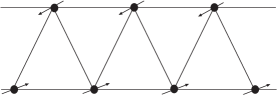
Figure 1: Spin chain: The multiferroic $LiCu_{2}O_{2}$ compound has pairs of $Cu^{2+}$ chains running parrallel to each other. Each chain is separated from the other by $b/2$ and forms the zig-zag triangular ladder structure shown in the figure. The black dots in the figure represent the magnetic $Cu^{2+}$ ions. These ions carry a spin-1/2 indicated by the arrow in the figure. The ladder is directed along the crystallographic $b$-axis.

The magnetic structure of $LiCu_{2}O_{2}$ has been determined from the neutron scattering experiments Masuda et al. (2004). The magnetic modulation vector obtained from these experiments is $\vec{Q}=(0.5\frac{2\pi}{a},\frac{2\pi\xi}{b},0)$ where $\xi=0.174$ is the spiral modulation along the chain direction. The letters $a,b,$ and $c$ represent the lattice constants of the simple orthorhombic crystal structure as mentioned earlier. Along the $a$-axis there is antiferromagnetic order and along the $b$-axis there is a spiral order. Succesive spins on each rung are almost parallel to each other with each spin being rotated relative to each other by an angle $\alpha=2\pi\xi$. Within each double chain any nearest-neighbor spins from opposite legs are almost antiparallel and form an angle $\alpha/2=\pi\xi$. Neutron diffraction experiments Masuda et al. (2004) conclude that rotating spins lie in the $bc$ plane out .

\psfrag{a}{$a$}\psfrag{c}{$c$}\psfrag{1}{$S_{1}$}\psfrag{2}{$S_{2}$}\psfrag{3}{$S_{3}$}\psfrag{4}{$S_{4}$}\includegraphics[width=144.54pt]{MagneticUnitCell.EPS}

(a) Magnetic unit cell

\psfrag{b}{$b$}\psfrag{c}{$c$}\psfrag{B}{$b/2$}\psfrag{-B}{$-b/2$}\psfrag{1}{$S_{1}$}\psfrag{2}{$S_{2}$}\psfrag{3}{$S_{3}$}\psfrag{4}{$S_{4}$}\includegraphics[width=144.54pt]{SideViewUnitCell.EPS}

(b) Side View of the unit cell

Figure 2: The dashed and the bold line indicates the bond between the $Cu^{2+}$ ions forming the zigzag chain.(a) Magnetic unit cell. The four black dots represent $Cu^{2+}$ ions. (b) Side view of the same magnetic unit cell. The center of inversion is situated halfway between the two $Cu^{2+}$ ions. These ladders are separated from each other by the non-magnetic $Li^{+}$ ions (distributed along the crystallographic $a$-axis) and by the layers of nonmagnetic $Cu^{+}$ ions (distributed along the crystallographic $c$-axis).

II.2 Experimental evidence of inter-chain coupling

The present theoretical formulation of spiral ferroelectrics do not consider the role of inter-chain coupling. For the $LiCu_{2}O_{2}$ compound, a spiral ferroelectric, there is experimental evidence from the Raman scattering experiment of Choi et.al. Choi et al. (2004) which suggests the presence of inter-chain interactions. Referring to Fig. 1 of their paper one can clearly observe that similar peaks are observed for both the parallel $(xx)$ and crossed polarizations $(xy)$. This indicates that inter-chain effects are important and should be considered in the theoretical formulation of $LiCu_{2}O_{2}$. Similar behavior has also been observed in the Na-analog compound $NaCu_{2}O_{2}$ Capogna et al. (2005); Choi et al. (2006). In this article we provide a theoretical justification using group theory for this important experimental observation. We also construct a phenomenological theory considering the effects of inter-chain coupling in multiferroic compounds.

III Symmetry operations of the lattice and magnetic structure

The goal of this section is to find a physically appropriate form for the magnetoelectric coupling in $LiCu_{2}O_{2}$ subject to the symmetry constraints of the magnetic structure. Physically such a term should conserve translational symmetry, space inversion symmetry, and time reversal symmetry. Phenomenological models Mostovoy (2006) are based on these considerations only. These models assume that a single unit cell of the lattice is a point in the system without any structure. An appropriate realistic model in these cases should include all the inequivalent atoms (considering both the type and location of the ion in space) in a single magnetic unit cell. This allows for the possibility to include more degrees of freedom. For example, in the LiCu₂O₂ case there are four spatially inequivalent magnetic ions in the magnetic unit cell that we should consider. They are denoted as $\vec{S}_{1}$, $\vec{S}_{2}$, $\vec{S}_{3}$, and $\vec{S}_{4}$ respectively (see Fig. 2).

As the number of possible forms of the magnetoelectric coupling increases rapidly with the degrees of freedom such a detailed model seems too complicated to be useful. However there are symmetry constraints which help to simplify the situation. These constraints should be obeyed by any term in the Hamiltonian including the magnetoelectric coupling term. The terms should be invariant under the lattice symmetry operations and time reversal symmetry. The lowest order magnetoelectric coupling which preserves time reversal symmetry is a trilinear term. It is linear in the electric polarization and bilinear in the magnetic order parameters. To simplify the discussion, we consider the coupling terms that involve the uniform spontaneous electric polarization, $\vec{P}$, and not those including the modulations of the polarization. The overall polarization has been experimentally measured and confirmed. The general magnetoelectric coupling is

$$H_{ME}=\lambda\sum_{\alpha\beta\gamma}P^{\alpha}\sum_{ij}\sum_{\vec{R}\vec{R}^{\prime}}C_{ij;\alpha\beta\gamma}(\vec{R}-\vec{R}^{\prime})S^{\beta}_{i}(\vec{R})S^{\gamma}_{j}(\vec{R}^{\prime})$$ (1)

where $\alpha,\;\beta,\;\gamma=x,\;y,\;z;$ $i,\;j=1,\;2,\;3,\;4,$ and $\vec{R}$ denotes the position of the unit cell. The magnetic structure in the compound can be written as $S^{\alpha}_{i}(\vec{R})=S^{\alpha}_{i}(\vec{Q})\exp(i\vec{Q}\cdot\vec{R})+c.c$. Substituting this expression into the above Hamiltonian we have

$$H_{ME}=\lambda\sum_{\alpha\beta\gamma}P^{\alpha}\sum_{ij}(C_{ij;\alpha\beta\gamma}(\vec{Q})S^{\beta}_{i}(\vec{Q})S^{\gamma}_{j}(-\vec{Q})+c.c)$$ (2)

where $C_{ij;\alpha\beta\gamma}(\vec{Q})$ is the Fourier transform of $C_{ij;\alpha\beta\gamma}(\vec{R}-\vec{R}^{\prime})$.

Not every term in the above magnetoelectric coupling conserves all the symmetries. Only certain linear combinations do. Specifically we are interested in the lattice symmetry operations that conserve the magnetic structure with the magnetic propagation vector $\vec{Q}$. From group representation theory we know that these operations constitute a subgroup of the full symmetry group of the lattice for which we have one (and only one) two-dimensional representation, $E$, $2_{b}$,$m_{c}$ and $m_{c}2_{b}$, all being two-by-two matrices . The lattice symmetry operations which preserve the magnetic structure and the magnetic propagation vector $\vec{Q}$ are listed in Table 1

Table 1: Lattice symmetry operations which preserve the magnetic structure and in turn the magnetic propagation vector- $\vec{Q}$. The identity operation is represented by $E$. A two-fold rotation about the crystallographic $b$-axis is represented by $2_{b}$. A reflection about the $c$-axis is denoted by $m_{c}$ and finally a combination of the the rotation-reflection by $m_{c}2_{b}$.

E${\bf r}=(x,y,z)$
$2_{b}{\bf r}=({\overline{x}},y+1/2,{\overline{z}})$
$m_{c}{\bf r}=(x-1/2,y,{\overline{z}}-1/2)$
$m_{c}2_{b}{\bf r}=({\overline{x}}-1/2,y+1/2,z-1/2)$

The two dimensional representations are given by

$$E=\left(\begin{array}[]{cc}1&0\\ 0&1\end{array}\right);2_{b}=\left(\begin{array}[]{cc}-e^{-iqb/2}&0\\ 0&e^{-iqb/2}\end{array}\right)$$ (7)

$$m_{c}=\left(\begin{array}[]{cc}0&-1\\ 1&0\end{array}\right);m_{c}2_{b}=\left(\begin{array}[]{cc}0&-e^{-iqb/2}\\ -e^{-iqb/2}&0\end{array}\right)$$ (12)

For the above representation we can find groups of symmetry adapted variables which are transformed according to the representation under the symmetry operations. These variables can be constructed as follows: a symmetry adapted variable is a column vector (two-dimensional in this case) whose elements are a linear combination of the original magnetic variables - $S_{i}^{\alpha}(\vec{Q})$’s. The variables transform under any operation of the subgroup in the same way they transform if left-multiplied by the corresponding matrix for the same operation. These variables can be computed for the $LiCu_{2}O_{2}$ case after deducing the transformation tables (see Table 2 and Table 3) of all the members of the symmetry subgroup.

Table 2: Symmetry operation: $2_{b}$, two-fold rotation about the crystallographic $b$-axis. In LiCu₂O₂ there are four spatially inequivalent magnetic ions in the magnetic unit cell. They are denoted as $\vec{S}_{1}$, $\vec{S}_{2}$, $\vec{S}_{3}$, and $\vec{S}_{4}$ respectively (see Fig. 2). The subscripts $a,b,$ and $c$ denote the components along those crystallographic axis.

$S_{1}$	$S_{2}$	$S_{3}$	$S_{4}$
$S^{{}^{\prime}}_{1a}=-S_{3a}e^{-iqb/2}$	$S^{{}^{\prime}}_{2a}=-S_{4a}e^{-iqb/2}$	$S^{{}^{\prime}}_{3a}=-S_{1a}$	$S^{{}^{\prime}}_{4a}=-S_{2a}$
$S^{{}^{\prime}}_{1b}=-S_{3b}e^{-iqb/2}$	$S^{{}^{\prime}}_{2b}=S_{4b}e^{-iqb/2}$	$S^{{}^{\prime}}_{3b}=S_{1b}$	$S^{{}^{\prime}}_{4b}=S_{2b}$
$S^{{}^{\prime}}_{1c}=-S_{3c}e^{-iqb/2}$	$S^{{}^{\prime}}_{2c}=-S_{4c}e^{-iqb/2}$	$S^{{}^{\prime}}_{3c}=-S_{1c}$	$S^{{}^{\prime}}_{4c}=-S_{2c}$

Table 3: Symmetry operation: $m_{c}$, reflection about the crystallographic $c$-axis. In LiCu₂O₂ there are four spatially inequivalent magnetic ions in the magnetic unit cell. They are denoted as $\vec{S}_{1}$, $\vec{S}_{2}$, $\vec{S}_{3}$, and $\vec{S}_{4}$ respectively (see Fig. 2). The subscripts $a,b,$ and $c$ denote the components along those crystallographic axis.

$S_{1}$	$S_{2}$	$S_{3}$	$S_{4}$
$S^{{}^{\prime}}_{1a}=-S_{2a}$	$S^{{}^{\prime}}_{2a}=S_{1a}$	$S^{{}^{\prime}}_{3a}=S_{4a}$	$S^{{}^{\prime}}_{4a}=-S_{3a}$
$S^{{}^{\prime}}_{1b}=-S_{2b}$	$S^{{}^{\prime}}_{2b}=S_{1b}$	$S^{{}^{\prime}}_{3b}=S_{4b}$	$S^{{}^{\prime}}_{4b}=-S_{3b}$
$S^{{}^{\prime}}_{1c}=S_{2c}$	$S^{{}^{\prime}}_{2c}=-S_{1c}$	$S^{{}^{\prime}}_{3c}=-S_{4c}$	$S^{{}^{\prime}}_{4c}=-S_{3c}$

As a result six groups of symmetry adapted variables are found, that is, twelve elements in total. The number of symmetry adapted vectors can also be deduced if we notice the fact that all of their elements should make a new basis for the magnetic structure which requires the total number of elements to be twelve, the same as the original $S_{i}^{\alpha}$’s, and the total number of vectors to be six. We divide them into two sets as listed below. The groups of symmetry adapted variables are

$$\mathcal{S}^{(1)}=\left\{\left(\begin{array}[]{c}S_{1a}+e^{-iqb/2}S_{3a}\\ S_{2a}-e^{-iqb/2}S_{4a}\end{array}\right),\left(\begin{array}[]{c}S_{1b}-e^{-iqb/2}S_{3b}\\ S_{2b}+e^{-iqb/2}S_{4b}\end{array}\right),\left(\begin{array}[]{c}S_{2c}+e^{-iqb/2}S_{4c}\\ S_{1c}-e^{-iqb/2}S_{3c}\end{array}\right)\right\}$$ (19)

$$\mathcal{S}^{(2)}=\left\{\left(\begin{array}[]{c}S_{2a}+e^{-iqb/2}S_{4a}\\ -S_{1a}+e^{-iqb/2}S_{4a}\end{array}\right),\left(\begin{array}[]{c}S_{2b}-e^{-iqb/2}S_{4b}\\ -S_{1b}-e^{-iqb/2}S_{3b}\end{array}\right),\left(\begin{array}[]{c}S_{1c}+e^{-iqb/2}S_{3c}\\ -S_{2c}+e^{-iqb/2}S_{4c}\end{array}\right)\right\}$$ (26)

Using the properties of the symmetry adapted variables we have

$$\mathcal{S}^{(i){\dagger}}_{\beta}M_{ij;\beta\gamma}\mathcal{S}^{(j)}_{\gamma}\stackrel{{\scriptstyle{2_{b}}}}{{\rightharpoonup}}\mathcal{S}^{(i){\dagger}}_{\beta}(m_{2_{b}})^{\dagger}M_{ij;\beta\gamma}m_{2_{b}}\mathcal{S}^{(j)}_{\gamma}=\mathcal{S}^{(i){\dagger}}_{\beta}(\sigma_{z}M_{ij;\beta\gamma}\sigma_{z})\mathcal{S}^{(j)}_{\gamma}$$ (27)

$$\mathcal{S}^{(i){\dagger}}_{\beta}M_{ij;\beta\gamma}\mathcal{S}^{(j)}_{\gamma}\stackrel{{\scriptstyle{m_{c}}}}{{\rightharpoonup}}\mathcal{S}^{(i){\dagger}}_{\beta}(m_{m_{c}})^{\dagger}M_{ij;\beta\gamma}m_{m_{c}}\mathcal{S}^{(j)}_{\gamma}=\mathcal{S}^{(i){\dagger}}_{\beta}(\sigma_{y}M_{ij;\beta\gamma}\sigma_{y})\mathcal{S}^{(j)}_{\gamma}.$$ (28)

Hereafter we suppress the argument of $S$. We will consider $S$ to be $S(\vec{Q})$ and $S^{+}$ to be $S(-\vec{Q})$. Having found the symmetry adapted variables, we put the magnetoelectric coupling in the following general form

$$H_{ME}=\lambda\sum_{\alpha}P^{\alpha}\sum_{i,j;\beta,\gamma}\mathcal{S}^{(i){\dagger}}_{\beta}M_{ij;\beta\gamma}\mathcal{S}^{(j)}_{\gamma}+c.c.$$ (29)

where $i,\;j=1,\;2$ and $M$ is an arbitrary two-by-twocoupling matrix. Using the properties of the symmetry adapted variables we have

$$\mathcal{S}^{(i){\dagger}}_{\beta}M_{ij;\beta\gamma}\mathcal{S}^{(j)}_{\gamma}\stackrel{{\scriptstyle{2_{b}}}}{{\rightharpoonup}}\mathcal{S}^{(i){\dagger}}_{\beta}(m_{2_{b}})^{\dagger}M_{ij;\beta\gamma}m_{2_{b}}\mathcal{S}^{(j)}_{\gamma}=\mathcal{S}^{(i){\dagger}}_{\beta}(\sigma_{z}M_{ij;\beta\gamma}\sigma_{z})\mathcal{S}^{(j)}_{\gamma}$$ (30)

$$\mathcal{S}^{(i){\dagger}}_{\beta}M_{ij;\beta\gamma}\mathcal{S}^{(j)}_{\gamma}\stackrel{{\scriptstyle{m_{c}}}}{{\rightharpoonup}}\mathcal{S}^{(i){\dagger}}_{\beta}(m_{m_{c}})^{\dagger}M_{ij;\beta\gamma}m_{m_{c}}\mathcal{S}^{(j)}_{\gamma}=\mathcal{S}^{(i){\dagger}}_{\beta}(\sigma_{y}M_{ij;\beta\gamma}\sigma_{y})\mathcal{S}^{(j)}_{\gamma}$$ (31)

Now we can apply the stated constraints to find all the possible forms of the magnetoelectric coupling.

1. Time reversal symmetry: The expression above with its tri-linearity automatically includes time reversal symmetry.

2. Lattice symmetry: We focus on the subgroup of the lattice symmetry operations. All three components of the electric polarization behave differently under the symmetry operations. We discuss each case separately. In the following we explicitly work out the case for $P_{c}$ and simply list the result for the other two components. The symmetry properties of $P_{c}$ under the lattice symmetry operations are $P_{c}\stackrel{{\scriptstyle m_{c}}}{{\rightarrow}}-P_{c}$, $P_{c}\stackrel{{\scriptstyle 2_{b}}}{{\rightarrow}}-P_{c}$, $P_{c}\stackrel{{\scriptstyle I}}{{\rightarrow}}-P_{c}$. From the overall invariance of the trilinear coupling we require that $M_{ij;\beta\gamma}$ anti-commute with both $\sigma_{y}$ and $\sigma_{z}$. From this we can infer that $M_{ij}$ should be proportional to $\sigma_{x}$ to preserve the invariance under symmetry operations. A similar procedure can be applied to find the appropriate $M_{ij}$’s for $P_{a}$ and $P_{b}$. The result can be summarized as follows: for $P_{a}$, $M_{ij}\propto\sigma_{y}$; for $P_{b}$, $M_{ij}\propto 1$; for $P_{c}$, $M_{ij}\propto\sigma_{x}$. Later we will prove that the constant of proportionality can be either real or purely imaginary based on space inversion symmetry arguments.

3. Inversion symmetry: Inversion operation is not a member of the subgroup of the symmetry operations that conserve the magnetic propagation vector $\vec{Q}$. Therefore it cannot be represented by a matrix acting on the symmetry adapted variables. The mapping for space inversion operation is

   $$S_{1}^{\alpha}(q)\rightarrow S_{3}^{\alpha}(-q),\;S_{2}^{\alpha}(q)\rightarrow S_{4}^{\alpha}(-q)$$ (32)

   $$S_{3}^{\alpha}(q)\rightarrow S_{1}^{\alpha}(-q),\;S_{4}^{\alpha}(q)\rightarrow S_{2}^{\alpha}(-q)$$ (33)

   where $\alpha$ denotes the spin component. With this mapping we obtain the expression for the inversion operation in terms of the symmetry adapted variables as

   $$I\cdot\mathcal{S}^{(i)}_{b}=\left(\begin{array}[]{cc}-e^{-iqb/2}&0\\ 0&e^{-iqb/2}\end{array}\right)\mathcal{S}^{(i)*}_{b}$$ (36)

   $$I\cdot\mathcal{S}^{(i)}_{\alpha}=\left(\begin{array}[]{cc}e^{-iqb/2}&0\\ 0&-e^{-iqb/2}\end{array}\right)\mathcal{S}^{(i)*}_{\alpha}$$ (39)

   where $\alpha=a,c$ and $i=1,2$ are the indices for the symmetry adapted variables. Below we explicitly work out the case for $P_{c}$ and list the result for the other two components of electric polarization. We have

   $$P_{c}\mathcal{S}^{(i){\dagger}}_{\beta}\sigma_{x}\mathcal{S}^{(j)}_{\gamma}\stackrel{{\scriptstyle I}}{{\rightharpoonup}}(-P_{c})(\mathcal{S}^{(i)T}_{\beta}\sigma_{z}\sigma_{x}\sigma_{z}\mathcal{S}^{(j)*}_{\gamma})=P_{c}(\mathcal{S}^{(i){\dagger}}_{\beta}\sigma_{x}\mathcal{S}^{(j)})^{*},$$ (40)

   if $\beta,\;\gamma=a,\;c$ or $\beta=\gamma=b$, and

   $$P_{c}\mathcal{S}^{(i){\dagger}}_{\beta}\sigma_{x}\mathcal{S}^{(j)}_{\gamma}\stackrel{{\scriptstyle I}}{{\rightharpoonup}}(-P_{c})(-\mathcal{S}^{(i)T}_{\beta}\sigma_{z}\sigma_{x}\sigma_{z}\mathcal{S}^{(j)*}_{\gamma})=-P_{c}(\mathcal{S}^{(i){\dagger}}_{\beta}\sigma_{x}\mathcal{S}^{(j)}_{\gamma})^{*},$$ (41)

   if one and only one of $\beta$ and $\gamma$ is $b$. The electric polarization and the total Hamiltonian must be real making the proportionality constant in the first case real and in the second case purely imaginary. The complete result is summarized below. It shows that there are only six generic terms that do not violate any of the symmetries of the system

   $$P_{a}(\mathcal{S}^{(i){\dagger}}_{\beta}\sigma_{y}\mathcal{S}^{(j)}_{\gamma}+c.c)$$ (42)

   $$P_{b}(\mathcal{S}^{(i){\dagger}}_{\beta}\mathcal{S}^{(j)}_{\gamma}+c.c)$$ (43)

   $$P_{c}(\mathcal{S}^{(i){\dagger}}_{\beta}\sigma_{x}\mathcal{S}^{(j)}_{\gamma}+c.c)$$ (44)

   if $\beta,\gamma=a,c$ or $\beta=\gamma=b$, and

   $$iP_{a}(\mathcal{S}^{(i){\dagger}}_{\beta}\sigma_{y}\mathcal{S}^{(j)}_{\gamma}-c.c)$$ (45)

   $$iP_{b}(\mathcal{S}^{(i){\dagger}}_{\beta}\mathcal{S}^{(j)}_{\gamma}-c.c)$$ (46)

   $$iP_{c}(\mathcal{S}^{(i){\dagger}}_{\beta}\sigma_{x}\mathcal{S}^{(j)}_{\gamma}-c.c)$$ (47)

   if one and only one of $\beta$ and $\gamma$ is $b$.

To summarize our work up to this point we have exhausted all possible forms of magnetoelectric coupling that are invariant under (1) time reversal, (2) space inversion, and (3) all the lattice symmetry operations that conserve the magnetic propagation vector by using the symmetry adapted variables.

IV Phenomenological magnetization model

A simplified expression for the phenomenological model can be obtained if we observe first that ferroelectricity coexists with the non-collinear magnetic structure. This suggests that terms with $\beta=\gamma$ can be excluded. Second, the polarization along the $b$-axis is not observed. Therefore, the couplings with $P_{b}$ need not be considered. Third, the magnetic moments on the four Cu²⁺ atoms, assumed to be independent variables in our theoretical formulation, form two zigzag chains Berger et al. (1991); Zvyagin et al. (2002); Roessli et al. (2001) extended in the $b$-direction on each of which a spin density wave with a propagation vector $q$ along the $b$-axis exists. To be specific, in Fig. 1, they propose that $S_{2}$ and $S_{4}$ are on one zigzag chain and $S_{1}$ and $S_{3}$ in the adjacent unit cell are on another zigzag chain. This observation drastically simplifies the expression of magnetoelectric coupling as

$$S_{1}^{\alpha}=e^{-iqb/2}S_{3}^{\alpha}$$ (48)

$$S_{2}^{\alpha}=-e^{-iqb/2}S_{4}^{\alpha}$$ (49)

These relations reduce the symmetry adapted variables to their final form as displayed in Eq. 72. Considering the fact that $S_{2a}=-e^{-iqb/2}S_{4a}$ and $S_{1b}=e^{-iqb/2}S_{3b}$ the symmetry adapted variables $\mathcal{S}^{(1)}$ and $\mathcal{S}^{(2)}$ become

$$\mathcal{S}^{(1)}=\left\{\left(\begin{array}[]{c}2e^{-iqb/2}S_{3a}\\ -2e^{-iqb/2}S_{4a}\end{array}\right),\left(\begin{array}[]{c}0\\ 0\end{array}\right),\left(\begin{array}[]{c}0\\ 0\end{array}\right)\right\}$$ (56)

$$\mathcal{S}^{(2)}=\left\{\left(\begin{array}[]{c}0\\ 0\end{array}\right),\left(\begin{array}[]{c}-2e^{-iqb/2}S_{4b}\\ -2e^{-iqb/2}S_{3b}\end{array}\right),\left(\begin{array}[]{c}2e^{-iqb/2}S_{3c}\\ 2e^{-iqb/2}S_{4c}\end{array}\right)\right\}$$ (64)

All the magnetoelectric couplings terms can be enumerated in terms of the symmetry adapted variables by using the above two equations. After the insertion of Eqs. 48 and 49 three of the six symmetry adapted variables reduce to zero. We can instead take the reduced symmetry adapted variable as

$$\vec{\mathcal{S}}=\left\{\left(\begin{array}[]{c}S^{(1)}_{a}\\ -S^{(2)}_{a}\\ \end{array}\right),\left(\begin{array}[]{c}-S^{(2)}_{b}\\ -S^{(1)}_{b}\\ \end{array}\right),\left(\begin{array}[]{c}S^{(1)}_{c}\\ S^{(2)}_{c}\\ \end{array}\right)\right\}$$ (72)

where the superfix denotes the chain number to which the spin belongs and the argument of the $S$’s are suppressed. However one should bear in mind that all the $S$’s are Fourier components and in general complex numbers.

IV.1 Intra-chain interaction terms

First let us enumerate all the intra-chain couplings that couple to $P_{c}$ and $P_{a}$. Since $P_{b}$ has not been observed under any conditions we ignore it in our theoretical consideration. These couplings are

$$iP_{c}(S^{(1)*}_{b}S^{(1)}_{c,a}-c.c.\pm(1)\rightarrow(2))$$ (73)

and

$$P_{a}(S^{(1)*}_{b}S^{(1)}_{c,a}+c.c.\mp(1)\rightarrow(2))$$ (74)

where the upper sign in the $\pm$ ($\mp$) is for the case when the subscript is $c$.

Our calculations show that an existing phenomenological theory Mostovoy (2006) for a spiral ferroelectric material in which only intra-chain interactions are included does not suitably explain the present system of interest. We demostrate through our calculations that some of the unexplained experimental facts may be ascribed to inter-chain interactions generated as a result of considering the details of the magnetic unit cell. We also show that not all the intra-chain and the inter-chain terms have the usual $\vec{P}\cdot[(\vec{M}\cdot\vec{\nabla})\vec{M}-(\vec{\nabla}\cdot\vec{M})\vec{M}]$ phenomenological form.

In the previous theory it is assumed that the electric polarization along the $c$-axis can be explained by its coupling with a cycloidal spin density wave on the $bc$-plane. Referring to Eq. 44 one finds that $P_{c}$ must be coupled to $S_{4b}S_{4c}^{*}+S_{3b}S_{3c}^{*}+c.c.$. As we know from above that $\vec{S}_{4}$ and $\vec{S}_{3}$ are the order parameters of different zigzag chains, we conclude that in this theory, the ferroelectric order $P_{c}$ couples to bilinear products inside a zigzag chain. Furthermore, when the magnetic field is applied along the $b$-axis, $P_{a}$ can also be induced, and it is explained by its coupling to a cycloidal spin density wave in the $ab$-plane. Using Eq. 42 we know that $P_{a}$ can only couple to $S_{4a}S_{4b}^{*}+S_{3a}S_{3b}^{*}+c.c.$ which is a product inside a single zigzag chain. Following this line of reasoning one easily sees that at least some unexplained multiferroic properties of the system must come from magnetoelectric couplings that involves more than one chain, that is, an inter-chain coupling term.

The physical picture of ferroelectricity induced by twisted magnetism has been widely recognized in multiferroic theories Mostovoy (2006). Through our calculation we point out that this physical picture is based on a single chain one-dimensional physics and has to modified to include inter-chain interaction. This observation is based on symmetry arguments and therefore promises to be independent of the specific form of interaction.

In transforming the above expressions, which are the Fourier components, to an expression in the real space, one should notice that a imaginary unit $i$ corresponds to an odd number of derivatives while the absence of an $i$ corresponds to an even number of derivatives. Therefore, if we only consider the lowest order in the continuous limit the above expressions can be written as

$$\lambda_{c}P_{c}(S^{(1)}_{b}(y)\partial_{y}S^{(1)}_{c,a}(y)-\partial_{y}S^{(1)}_{b}(y)S^{(1)}_{c,a}(y)$$

$$\pm(1)\rightarrow(2))$$

and

$$P_{a}(S^{(1)}_{b}(y)S^{(1)}_{c,a}(y)\mp(1)\rightarrow(2))$$ (76)

If the magnetic structure is a cycloidal spiral on the $bc$-plane we can easily see that $P_{c}\neq 0$ which is in accord with the phenomenological theory. The coupling in front of the $P_{c}$ component of polarization is dependent on the magnetic field along the $a$-axis and is sensitive to it. A discrepancy with the intra-chain phenomenlogical theory occurs when we consider the observed ferroelectricity flop from the $c$-axis to the the $a$-axis. In the phenomenological theory it is explained as derived from a spin flop from the cycloid on the $bc$-plane to the $ab$-plane. However if we consider a magnetic structure such as $\vec{S}(x)=S(\cos(qx),\sin(qx),0)$ we find that $P_{a}$ gives a modulated value and therefore averages to zero. Since the starting point from group theory is more general we believe that the phenomenological expression for the magnetoelectric coupling

$$\vec{P}\cdot[(\vec{M}\cdot\vec{\nabla})\vec{M}-(\vec{\nabla}\cdot\vec{M})\vec{M}]$$ (77)

does not capture the entire physical picture. Specifically in this case the $P_{c}[(\vec{M}\cdot\vec{\nabla})\vec{M}-(\vec{\nabla}\cdot\vec{M})\vec{M}]_{c}$ has the correct form while the expression for $P_{a}[(\vec{M}\cdot\vec{\nabla})\vec{M}-(\vec{\nabla}\cdot\vec{M})\vec{M}]_{a}$ is invalid atleast for the $LiCu_{2}O_{2}$ case. The derivation of the phenomenological theory Mostovoy (2006) assumes certain general symmetries of the Hamiltonian to construct the magnetoelectric coupling for $P_{a}$ and $P_{c}$. Based on such an argument there is no reason for the coupling to be different.

The starting point of the phenomenological theory Mostovoy (2006) considers each unit cell as a single site with magnetization $M$. This assumption does not hold if the little group of the lattice symmetry operations has no one-dimensional representation. If the system can be effectively described by only the unit cell magnetization $M$, then all the little group operations should commute and there must exist at least one one-dimensional representation. In the case of multiferroics such as $RMnO_{3}$ Kimura et al. (2003a, b) and $Ni_{3}V_{2}O_{8}$ Lawes et al. (2005) there are one-dimensional representations and the phenomenological theory provides a correct description Harris and Lawes (2005). For other multiferroic systems such as $R$Mn₂O₅ and $LiCu_{2}$O₂ only two-dimensional representations exist because of the antiferromagnetic structure along the $a$-axis. As a result the conventional phenomenological theory doesnot apply. From the above discussion we clearly see that the intrinsic structure of the unit cell is important and therefore must be taken into consideration.

IV.2 Inter chain interactions

From the expressions for the intra-chain terms we can conclude that an explanation for the net magnetization along the $a$-axis cannot be obtained within the intra-chain theory. We therefore go beyond the scope of that theory and include the effects of inter-chain coupling. Since there are several terms involved we first focus on those that couple to $P_{c}$. These expressions are

$$P_{c}(\vec{S^{(1)}}\times\vec{S^{(2)}})_{b}$$ (78)

$$P_{c}(\lambda_{a}S^{(1)}_{a}S^{(2)}_{a}+\lambda_{b}S^{(1)}_{b}S^{(2)}_{b}+\lambda_{c}S^{(1)}_{c}S^{(2)}_{b})$$ (79)

where the $\lambda$’s are arbitrary constants. Physically the first term could induce a polarization when the spins are aligned on the $ac$-plane and $\vec{S^{(1)}}\bot\vec{S^{(2)}}$. If the $\lambda$’s are close to each other the second term can be viewed as $\lambda P_{c}(\vec{S}_{1}\cdot\vec{S}_{2})$. This term is minimized with a collinear spin arrangement. The terms that couple to $P_{a}$ are

$$P_{a}(\vec{S^{(1)}}\times\partial_{y}\vec{S^{(2)}}+\vec{S^{(2)}}\times\partial_{y}\vec{S^{(1)}})_{b}$$ (80)

$$P_{a}(\beta_{a}S^{(1)}_{a}\partial_{y}S^{(2)}_{a}-\beta_{a}\partial_{y}S^{(1)}_{a}S^{(2)}_{a}+\beta_{b}S^{(1)}_{b}\partial_{y}S^{(2)}_{b}-\beta_{b}\partial_{y}S^{(1)}_{b}S^{(2)}_{b}+\beta_{c}S^{(1)}_{c}\partial_{y}S^{(2)}_{c}-\beta_{c}\partial_{y}S^{(1)}_{c}S^{(2)}_{c})$$ (81)

Same as above we can see that the first term induces a nonzero ferroelectricity with the alignment on the $ac$-plane and the collinearity between the two chains while the second term is minimized when $\vec{S^{(1)}}\bot\vec{S^{(2)}}$. The above group theory analysis yields the possible intra-chain and inter-chain magnetoelectric terms. The coupling parameters in the interactions cannot be determined without a proper understanding of the microscopic theory of the material compound and without improved experimental results.

V Effective Hamiltonian and electromagnon selection rules

In this section we conjecture a simple effective Hamiltonian which can explain the basic phenomena observed in the $LiCu_{2}O_{2}$ experiments Park et al. (2007). In particular we provide an explanation for the polarization flip in the presence of an external magnetic field. Furthermore, using the phenomenological Hamiltonian we also predict a selection rule to be obeyed by the hybrid excitations of phonon and magnon termed as electromagnons Sushkov et al. (2007) in the literature. It is hoped that these electromagnon excitations can be experimentally detected in future experiments.

V.1 Effective Hamiltonian

The effective Hamiltonian that we propose includes only two terms. One term involves the intra-chain coupling which is responsible for the electric polarization along the $c$-axis. The other term involves the inter-chain coupling that is responsible for the electric polarization along the $a$-axis. The magnetoelectric coupling Hamiltonian, $H_{em}$, is given by

$$H_{em}=\lambda_{c}P_{c}(\vec{S}^{(1)}\times\partial_{y}\vec{S}^{(1)}+\vec{S}^{(2)}\times\partial_{y}\vec{S}^{(2)})_{a}$$

$$+\lambda_{a}P_{a}(\vec{S}^{(1)}\times\partial_{y}\vec{S}^{(2)}+\vec{S}^{(2)}\times\partial_{y}\vec{S}^{(1)})_{b}$$ (82)

where the symbols have the same meaning as before. Both these terms satisfy the underlying lattice and magnetic symmetry requirements.

The proposed effective Hamiltonian explains the basic physics of the $LiCu_{2}O_{2}$ system. First, in the absence of any external magnetic field according to the neutron scattering experiments Masuda et al. (2004) the spins lie on the $bc$-plane. We have for the ground state spin configuration, $\vec{S}^{(1)}_{o}$ and $\vec{S}^{(2)}_{o}$, in the two chains

$$\vec{S}^{(1)}_{o}=S(0,\cos(qy),\sin(qy))$$ (83)

$$\vec{S}^{(2)}_{o}=S(0,\cos(qy+\delta\phi),\sin(qy+\delta\phi)$$ (84)

where $\delta\phi$ is the phase difference between the spin configurations of the two chains. Based on Eq. V.1 this spin configuration leads to an electric polarization along the $c$-axis

$$P_{c}\propto(\vec{S}^{(1)}\times\partial_{y}\vec{S}^{(1)}+\vec{S}^{(2)}\times\partial_{y}\vec{S}^{(2)})_{a}=const.$$ (85)

Second, in the presence of an applied magnetic field along the $b$-axis the spin should flip to the $ac$ plane when the field is larger than a certain critical value. This spin-flop transition is expected in a very general magnetic model with relatively isotropic couplings and spiral magnetism. This is similar to the spin-flop transition in the antiferromagnetic Heisenberg model in the presence of a Zeeman magnetic field. Therefore the expected ground state spin configuration in the two chains are

$$\vec{S}^{(1)}_{o}=S(\cos(qy),0,\sin(qy))$$ (86)

$$\vec{S}^{(2)}_{o}=S(\cos(qy+\delta\phi,0,\sin(qy+\delta\phi))$$ (87)

Based on Eq. V.1 this spin arrangement leads to an electric polarization along the $a$-axis when the spin structure in both the spin chains are in phase, that is, $\delta\phi=0$

$$P_{a}\propto(\vec{S}^{(1)}\times\partial_{y}\vec{S}^{(2)}+\vec{S}^{(2)}\times\partial_{y}\vec{S}^{(1)})_{b}=const.$$ (88)

The theoretical model developed above suggests that the polarization in the two crystallographic direction comes from two different types of coupling. The polarization along the $c$-axis arises from the intra-chain coupling while the polarization along the $a$-axis stems from the inter-chain coupling. Furthermore, in formulating this model we do not include strong anisotropy in the spin model to explain the flop transition of the electric polarization in the presence of an applied external magnetic field.

The proposed Hamiltonian explains the polarization flop by an applied magnetic field without introducing complicated anisotropic magnetic couplings Mostovoy (2006). The above model predicts explicit magnetic configurations corresponding to the polarization directions which can be verified in future experiments.

V.2 Electromagnon selection rule

Electromagnons are a combination of phonon and magnon excitations Sushkov et al. (2007). From the phenomenological model we can derive an explicit selection rule governing the electromagnons. The selection rule can be stated as follows: Electromagnetic waves that are polarized perpendicular to the bulk electric polarization can be absorbed. To be more specific in zero magnetic field only those electromagnetic waves that are polarized along the crystallographic $a$-axis can couple to the magnons. However, with an applied magnetic field along the $b$-axis only those waves polarized in the crystallographic $c$-axis can couple to the magnons.

The selection rules can be obtained in the following manner. We first consider the case with the external magnetic field absent. The dynamics of the system can be derived by assuming a small deviation in the ground state properties

$$\vec{P}=\vec{P}_{o}+\vec{u}$$ (89)

$$\vec{S}^{(1)}=\vec{S}^{(1)}_{o}+\delta\vec{S}^{(1)}$$ (90)

$$\vec{S}^{(2)}=\vec{S}^{(2)}_{o}+\delta\vec{S}^{(2)}$$ (91)

where $\vec{P}_{o}$, $\vec{S}^{(1)}_{o}$, and $\vec{S}^{(2)}_{o}$ are the ground state values and the small deviations are indicated by $\vec{u}$, $\delta\vec{S}^{(1)}$, and $\delta\vec{S}^{(2)}$. Energy minimization requires that the first order terms vanish in the ground state. We therefore study the second order terms in the perturbation expansion to see how the dynamical degrees of freedom are coupled. Also the spin being a length-preserving vector we know that $\delta\vec{S}_{i}\bot\vec{S}_{i0}$. Defining $\vec{n}_{1}=(0,\cos(qy),\sin(qy)),\;\vec{n}_{2}=(0,-\sin(qy),\cos(qy))$, we have $\delta\vec{S}_{1}=m^{(1)}_{1}\vec{n}_{2}+m^{(1)}_{2}\vec{a}$ (where $\vec{a}$ is the unit vector along the $a$-axis). We now consider the second order coupling that involves $\vec{u}_{c}$ and $\delta\vec{S}_{1}$ derived from Eq. V.1

$$u_{c}(\delta\vec{S}^{(1)}\times\partial_{y}\vec{S}^{(1)}_{o}-\partial_{y}\delta\vec{S}^{(1)}\times\vec{S}^{(1)}_{o})_{a}$$

$$=S^{2}u_{c}(q(m^{(1)}_{1}\vec{n}_{2}+m^{(1)}_{2}\vec{a})\times\vec{n}_{2}$$

$$-(\partial_{y}m^{(1)}_{1}\vec{n}_{2}-qm^{(1)}_{1}\vec{n}_{1}+\partial_{y}\vec{a})\times\vec{n}_{1})_{a}$$

$$=S^{2}\partial_{y}m_{1}u_{c}$$ (92)

In momentum space the above expression can be written as

$$S^{2}u_{c}(-\vec{k})(-ik_{y})m^{(1)}_{1}(\vec{k})$$ (93)

From this we infer that the zero mode phonon $u_{c}(\vec{k}=0)$ does not couple to the magnons. Therefore, if we compute the optical conductivity $\mbox{Im}G_{uu}(\vec{k}=0,\omega)$ in the lowest order (second order) the coupling does not contribute. This shows that when $P_{c}\neq 0$ the phonons along the same direction do not couple to the magnons. These phonons make no contribution to the electromagnons that may be observed in an optical conductivity measurement. However, the higher order terms are still coupled. A similar type of result can be obtained with the terms involving $\delta\vec{S}_{2}$. This verifies the first part of our selection rule by showing that when an electric polarization is present along the $c$-axis only the phonons polarized along the $a$-axis can couple to the magnons to generate the electromagnons.

The coupling between the phonons polarized along the $a$-axis and the magnons can be derived as follows. For $u_{a}$, from Eq. 82 we have

$$u_{a}(\delta\vec{S}_{1}\times\partial_{y}\vec{S}_{20}-\vec{S}_{20}\times\partial_{y}\delta\vec{S}_{1})_{b}$$

$$=S^{2}u_{a}(-q\cos(qy)m^{(1)}_{2}+\sin(qy)\partial_{y}m^{(1)}_{2})$$ (94)

Therefore the total effective Hamiltonian, $H^{eff}_{d}$, describing the dynamics of the phonon and the magnon can be written as

$$H^{eff}_{d}=\sum_{p}\{{h\omega_{0}}b^{\dagger}(p)b(p)+\frac{\rho p^{2}}{2}\sum_{i}m_{2}^{{\dagger}(i)}(p)m_{2}^{(i)}(p)+$$

$$\frac{\lambda_{a}S^{2}}{2}(b^{\dagger}(p+q)+b^{\dagger}(p-q))[-qm_{+}(p)-pm_{+}(p)]\}$$ (95)

where $h$ is the Planck’s constant, $\rho\sim J$ (the effective magnetic coupling strength in the magnetic chain), $q$ is the incommensurate wavevector, $\omega_{0}$ is the bare phonon energy, $b_{p}$ is phonon annihilation operator, and $m_{+}=\sum_{i}m^{(i)}_{2}$.

A qualitative understanding of the electromagnon frequency for the $LiCu_{2}O_{2}$ compound can be obtained by using a spinwave analysis. The analysis was done for the case when the optical phonon frequency is much larger than the magnon frequency of interest. This implies that if we measure the ac-conductivity versus frequency one will observe a peak at the frequency of the magnon. We should also note that two points justify the neglect of the dynamic lattice degrees of freedom, the displacement field $u$, for the $LiCu_{2}O_{2}$ system. First, the optical phonon frequency is much higher than the magnon frequency. Second, the magnetoelectric coupling is very small compared with to the other multiferroics, like the $113$ systems, making it unnecessary to explicitly include the dynamic degrees of freedom in the dielectric displacement Katsura et al. (2005). We now perform a standard spinwave analysis Katsura et al. (2005) about the ground state to find the frequency at the desired wavevector, $\vec{k}=\vec{Q}$.

The model Hamiltonian for $LiCu_{2}O_{2}$ proposed by Masuda et al. (2004) is

$$H=\sum_{i,j}(J_{1}\vec{S}_{i,j}\cdot\vec{S}_{i+1,j}+J_{2}\vec{S}_{i,j}\cdot\vec{S}_{i+2,j}$$

$$+J_{4}\vec{S}_{i,j}\cdot\vec{S}_{i+4,j}+J_{\perp}\vec{S}_{i,j}\cdot\vec{S}_{i,j+1})+DS_{\perp}^{2}.$$ (96)

Here we have included an easy plane anisotropy which generally exists due to the anisotropy of the lattice and this term favors the easy plane of spin alignment in the ground state, say, the bc-plane in zero field, but the ac-plane in a strong magnetic field along the b-axis. We solve for the spin wave dispersion. We employ the rotating frame of reference coordinate system to write the spin vector at any site relative to the other rotating one as

$$\vec{S}_{i,j}=S^{\xi}_{i,j}\vec{e}_{x}+[S^{\eta}_{i,j}\cos(\vec{Q}\cdot\vec{R}_{i,j})+S^{\zeta}_{i,j}\sin(\vec{Q}\cdot\vec{R}_{i,j})]\vec{e}_{y}$$

$$+[-S^{\eta}_{i,j}\sin(\vec{Q}\cdot\vec{R}_{i,j})+S^{\zeta}_{i,j}\cos(\vec{Q}\cdot\vec{R}_{i,j})]\vec{e}_{z}$$

In the above equation the magnetic propagation vector is given by $\vec{Q}=(\frac{\pi}{a},\frac{2\pi\xi}{b},0)$ where $\xi=0.174$ is the spiral modulation along the chain. Inserting the above form for the spin vector we recast the Hamiltonian in terms of $S^{\xi},S^{\eta}$ and $S^{\zeta}$ components. We then compute the effective magnetic field components using the formula $\vec{H}_{eff}=-\vec{\nabla}_{\vec{S}_{i,j}}H$. We then solve for the equation of motion for the spin components using the effective magnetic field equations and spin components in terms of the Holstein-Primakoff formalism listed below

$$S^{\xi}_{m,n}=\sqrt{\frac{S}{2}}(a_{m,n}+a^{*}_{m,n})$$ (98)

$$S^{\eta}_{m,n}=-i\sqrt{\frac{S}{2}}(a_{m,n}-a^{*}_{m,n})$$ (99)

The equations of motion are given by

$$\hbar{\stackrel{{\scriptstyle.}}{{S}}^{\xi}_{m,n}}=S^{\eta}_{m,n}H^{\zeta}_{eff}-S^{\zeta}_{m,n}H^{\eta}_{eff}$$ (100)

$$\hbar{\stackrel{{\scriptstyle.}}{{S}}^{\eta}_{m,n}}=S^{\zeta}_{m,n}H^{\xi}_{eff}-S^{\xi}_{m,n}H^{\zeta}_{eff}$$ (101)

where in the above equation we set $S^{\zeta}_{i,j}=S$ since it is the direction in which the spin average points. Using the equations for the effective magnetic field, the spin components, and finally Fourier transforming we obtain the dispersion as

$$-\frac{\hbar}{2S}\dot{S}^{\xi}(\vec{q})=S^{\eta}(\vec{q})(J(\vec{Q})-\frac{J(\vec{Q}+\vec{q})+J(\vec{Q}-\vec{q})}{2}),$$ (102)

$$-\frac{\hbar}{2S}\dot{S}^{\eta}(\vec{q})=S^{\xi}(\vec{q})(J(\vec{q})-J(\vec{Q})+D),$$ (103)

where we define $J(\vec{q})=J_{1}\cos(q_{b}b)+J_{2}\cos(2q_{b}b)+J_{4}\cos(4q_{b}b)+J_{\perp}\cos(q_{a}a)$ where $q_{a}$ and $q_{b}$ refer to the $a$ and $b$ components of the wavevector. From the equations above it is obvious that at $\vec{q}=\vec{Q}$ we have

$$\hbar\omega(\vec{Q})=2S\sqrt{(\frac{J(2\vec{Q})+J(0)}{2}-J(\vec{Q}))D}.$$ (104)

The electromagnon dispersion indicates that the frequency is proportional to the square root of the easy plane anisotropy, $D$. In zero field, the easy plane is the $bc$-plane. With an applied magnetic field along the $a$-axis, this field will effectively increase the anisotropy in the form of $D\sim D_{0}+H_{a}^{2}/2\rho$ Fang and Hu (2008), where $\rho$ is the spin stiffness. This should lead to a hardening of the electromagnon frequency (a right shift of the peak in the ac-conductivity measurement). If the magnetic field is applied along the $b$-axis, it effectively diminshes the easy plane anistropy in the form of $D\sim D_{0}-H_{b}^{2}/2\rho$. Therefore, one must observe the softening along with the increase of the magnetic field and at the point where the frequency becomes zero, the magnon mode becomes unstable and the spin-flop transition happens

The above mechanism explains the observed phase transition at a certain magnetic field along the $b$-axis as the destabilization of one electromagnon mode. In the high field phase, the spins are lying in the $ac$-plane, making the $ac$-plane an easy plane described by an anisotropy term. In this phase, further increasing the field along the $b$-axis will increase the easy plane anisotropy, whereas applying a field along the $a$-axis will decrease the anisotropy. Therefore, we predict that the electromagnon hardens with an increase of magnetic field along the $b$-axis, and softens with an increase of magnetic field along the $a$-axis. This is opposite to what we should see in the low field phase.

VI Summary and Conclusions

In this paper we analyze the possible types of magnetoelectric coupling in the recently studied multiferroic compound $LiCu_{2}O_{2}$. Based on a group theoretical analysis we construct a multi-order parameter phenomenological model for the double chain zig-zag structure. We show that a coupling involving the inter-chain magnetic structure and ferroelectricity is crucial in understanding the results of Park et.al. Park et al. (2007). This constructed model for the multiferroic $LiCu_{2}O_{2}$ compound can explain the polarization flop from the $c$-axis to the $a$-axis with the applied magnetic field along the $b$-axis. The model also makes specific selection rule predictions about the hybrid phonon and magnon excitations called electromagnons. We also predict that the electromagnon peaks measured in an $ac$-conductivity measurement are field dependent and behave in opposite ways in the $P//a$ phase and $P//c$ phase. However, since the value of the polarization in this material is rather weak it will require a very high resolution spectroscopy measurement to observe the electromagnons in the actual system.

The results in this paper suggest that the effective theory of magnetoelectric coupling is richer in a system described by multi-order parameters where several magnetoelectric coupling terms can be constructed, than that in a system described by a single order parameter. Similar physics has also been demonstrated for the $RMn_{2}O_{5}$Fang and Hu (2008) multiferroic system and it should be thoroughly investigated for the other materials.

The model we propose in this paper could be oversimplified. However, at present only a limited set of experimental results are available for this compound. We believe this phenomenological model is a first step towards understanding the unique and novel magnetoelectric coupling observed in the $LiCu_{2}O_{2}$ compound. It is open to future experiments to determine the relevance of the other magnetoelectric coupling terms which we derived in this paper based on a group theoretical calculation.

VII Acknowledgements

JP Hu acknowledges the extremely useful discussions with Prof. S.W. Cheong.

References

- Park et al. (2007) S. Park, Y. J. Choi, C. L. Zhang, and S.-W. Cheong, Phys. Rev. Lett. 98, 057601 (2007).
- Kimura et al. (2003a) T. Kimura, T. Goto, H. Shintani, K. Ishizaka, T. Arima, and Y. Tokura, Nature 426, 55 (2003a).
- Hur et al. (2004a) N. Hur, S. Park, P. A. Sharma, J. S. Ahn, S. Guha, and S. W. Cheong, Nature 429, 392 (2004a).
- Goto et al. (2004) T. Goto, T. Kimura, G. Lawes, A. P. Ramirez, and Y. Tokura, Phys. Rev. Lett. 92, 257201 (2004).
- Lottermoser et al. (2004) T. Lottermoser, T. Lonkai, U. Amann, D. Hohlwein, J. Ihringer, and M. Fiebig, Nature 430, 541 (2004).
- Lorenz et al. (2004) B. Lorenz, Y. Q. Wang, Y. Y. Sun, and C. W. Chu, Phys. Rev. B 70, 212412 (2004).
- Higashiyama et al. (2004) D. Higashiyama, S. Miyasaka, N. Kida, T. Arima, and Y. Tokura, Phys. Rev. B 70, 174405 (2004).
- Hill (2000) N. A. Hill, J. Phys. Chem. B 104, 6694 (2000).
- Fiebig (2005) M. Fiebig, J. Phys. D 38, R123 (2005).
- Khomskii (2006) D. I. Khomskii, J. Magn. Magn. Mater. 306, 1 (2006).
- Cheong and Mostovoy (2007) S. W. Cheong and M. Mostovoy, Nat. Mater. 6, 13 (2007).
- Kimura et al. (2003b) T. Kimura, S. Kawamoto, I. Yamada, M. Azuma, M. Takano, and Y. Tokura, Phys. Rev. B 67, 180401 (2003b).
- Kimura et al. (2005a) T. Kimura, G. Lawes, T. Goto, Y. Tokura, and A. P. Ramirez, Phys. Rev. B 71, 224425 (2005a).
- Hur et al. (2004b) N. Hur, S. Park, P. A. Sharma, S. Guha, and S.-W. Cheong, Phys. Rev. Lett. 93, 107207 (2004b).
- Kimura et al. (2006) T. Kimura, J. C. Lashley, and A. P. Ramirez, Phys. Rev. B 73, 220401 (2006).
- Yamasaki et al. (2006) Y. Yamasaki, S. Miyasaka, Y. Kaneko, J. P. He, T. Arima, and Y. Tokura, Phys. Rev. Lett. 96, 207204 (2006).
- Taniguchi et al. (2006) K. Taniguchi, N. Abe, T. Takenobu, Y. Iwasa, and T. Arima, Phys. Rev. Lett. 97, 097203 (2006).
- Lawes et al. (2005) G. Lawes, A. B. Harris, T. Kimura, N. Rogado, R. J. Cava, A. Aharony, O. Entin-Wohlman, T. Yildirim, M. Kenzelmann, C. Broholm, et al., Phys. Rev. Lett. 95, 087205 (2005).
- Kimura et al. (2005b) T. Kimura, G. Lawes, and A. P. Ramirez, Phys. Rev. Lett. 94, 137201 (2005b).
- (20) Private communications with Prof. S.W.Cheong. A correct identification of the crystal structure axes cannot be made unambiguously.
- Moskvin and Drechsler (2008) A. S. Moskvin and S. L. Drechsler (2008), arXiv.org:0801.1102.
- Moskvin et al. (2008) A. S. Moskvin, Y. D. Panov, and S. L. Drechsler (2008), arXiv.org:0801.1975.
- Katsura et al. (2005) H. Katsura, N. Nagaosa, and A. V. Balatsky, Phys. Rev. Lett. 95, 057205 (2005).
- Hu (2008) J. Hu, Phys. Rev. Lett. 100, 077202 (2008).
- Sergienko and Dagotto (2006) I. A. Sergienko and E. Dagotto, Phys. Rev. B 73, 094434 (2006).
- Mostovoy (2006) M. Mostovoy, Phys. Rev. Lett. 96, 067601 (2006).
- Harris and Lawes (2005) A. B. Harris and G. Lawes, cond-mat/0508617 (2005).
- Choi et al. (2004) K.-Y. Choi, S. A. Zvyagin, G. Cao, and P. Lemmens, Phys. Rev. B 69, 104421 (2004).
- Berger et al. (1991) R. Berger, A. Meetsma, S. van Smaalen, and M. Sundberg, J. Less-Common Met. 175, 119 (1991).
- Zvyagin et al. (2002) S. Zvyagin, G. Cao, Y. Xin, S. McCall, T. Caldwell, W. Moulton, L.-C. Brunel, A. Angerhofer, and J. E. Crow, Phys. Rev. B 66, 064424 (2002).
- Roessli et al. (2001) B. Roessli, U. Staubb, A. Amatoc, D. Herlachc, P. Pattisond, K. Sablinae, and G. A. Petrakovskiie, Physica B 296, 306 (2001).
- Masuda et al. (2004) T. Masuda, A. Zheludev, A. Bush, M. Markina, and A. Vasiliev, Phys. Rev. Lett. 92, 177201 (2004).
- (33) While the neutron diffraction experiments Masuda et al. (2004) conclude that rotating spins lie in one plane (), there is independent NMR studies Gippius et al. (2004) which show an out-of-plane component.
- Capogna et al. (2005) L. Capogna, M. Mayr, P. Horsch, M. Raichle, R. K. Kremer, M. Sofin, A. Maljuk, M. Jansen, and B. Keimer, Phys. Rev. B 71, 140402 (2005).
- Choi et al. (2006) K.-Y. Choi, V. P. Gnezdilov, P. Lemmens, L. Capogna, M. R. Johnson, M. Sofin, A. Maljuk, M. Jansen, and B. Keimer, Phys. Rev. B 73, 094409 (2006).
- Sushkov et al. (2007) A. B. Sushkov, R. V. Aguilar, S. Park, S.-W. Cheong, and H. D. Drew, Phys. Rev. Lett. 98, 027202 (2007).
- Fang and Hu (2008) C. Fang and J. Hu (2008), ”An effective model of magnetoelectricity in multiferroics RMn(2)O(5), to appear in Europhys. Lett.”.
- Gippius et al. (2004) A. A. Gippius, E. N. Morozova, A. S. Moskvin, A. V. Zalessky, A. A. Bush, M. Baenitz, H. Rosner, and S.-L. Drechsler, Phys. Rev. B 70, 020406 (2004).