Global Conservation Laws and Femtoscopy of Small Systems

Abstract

It is increasingly important to understand, in detail, two-pion correlations measured in $p+p$ and $d+A$ collisions. In particular, one wishes to understand the femtoscopic correlations, in order to compare to similar measurements in heavy ion collisions. However, in the low-multiplicity final states of these systems, global conservation laws generate significant $N$-body correlations which project onto the two-pion space in non-trivial ways and complicate the femtoscopic analysis. We discuss a formalism to calculate and account for these correlations in collisions dominated by a single particle species (e.g. pions). We also discuss effects on two-particle correlations between non-identical particles, the understanding of which may be important in the study of femtoscopic space-time asymmetries.

I INTRODUCTION

The unique and distinguishing feature of collisions between heavy ions is their large (relative to the confinement scale) size and the possibility to generate bulk systems which may be described in thermodynamic terms, allowing to discuss the Equation of State of strongly-interacting matter. The primary evidence for the creation of bulk matter at the highest energies Adams:2005dq ; Adcox:2004mh ; Back:2004je ; Arsene:2004fa is the existence of strong collective flow Ollitrault:1992bk . The dominant feature of flow is the correlation between space and momentum which it generates; thus, momentum-only observables such as $p_{T}$ spectra and azimuthal anisotropies Adams:2005dq ; Adcox:2004mh ; Back:2004je ; Arsene:2004fa represent only an indirect projection of the effect. Femtoscopic measurements access space as a function of particle momentum, thus providing the most direct probe of the most crucial feature of heavy ion collisions (c.f. e.g. Lisa:2005dd, ). In particular, flow is manifest by a negative correlation between the “HBT radius” and the transverse mass ($m_{T}$) of the particles Pratt:1984su .

Clearly, then, a detailed understanding of femtoscopic measurements in heavy ion collisions is crucial to proving the existence of, or probing the nature of, the bulk system generated in the collision. It is in fact possible to quantitatively interpret both the femtoscopic and momentum-only observations at RHIC– in A+A collisions– in consistent, flow-dominated models of the system (e.g. Retiere:2003kf, ). All seems well.

However, it is important to understand the system size dependence of the apparent bulk behavior. In this paper we discuss the possible complications in the comparison of large and small systems.

I.1 Hadron collisions as a reference to heavy ion collisions

One of the most exciting signals at RHIC is the modification of the jet structure due to the bulk medium. In particular leading particle distributions Adler:2003qi ; Adams:2003kv and azimuthal correlations Adler:2002tq in A+A collisions are strongly suppressed relative to those from p+p collisions, at high $p_{T}$.

Especially since low $p_{T}$ observables directly reflect the bulk medium, it is reasonable to ask whether similar comparisons between Au+Au and p+p collisions reveal comparable differences in the soft sector.

Common measurements of this type include total particle yields, $p_{T}$ spectra and azimuthal correlations ($v_{2}$). However, in each case, it is not clear if qualitative differences between small and large systems are observed. Quantum number conservation laws in small systems can strongly affect particle yields (e.g. Derreth:1985kk, ; Elze:1986db, ). However, modulo canonical suppression effects, equilibrium-based thermochemical fits to yields from p+p collisions Becattini:1997xx produce quite similar results to those from A+A collisions Braun-Munzinger:2001ip . Blast-wave fits Schnedermann:1993ws ; Retiere:2003kf to $p_{T}$ spectra from p+p collisions indicate sizable radial flow, though smaller than that seen in Au+Au collisions Adams:2003xp . Intrinsic anisotropies from p+p collisions are considered as non-flow contribution to azimuthal correlations in A+A. However, it is far from obvious that the finite values of $v_{2}$ from p+p collisions Adams:2004bi do not arise from collective flow in the p+p collision itself.

A Quark-Gluon Plasma is usually considered a form of matter. If a Quark-Gluon Plasma were created in p+p collisions, as suggested by Bjorken Bjorken:1982tu , would it display bulk properties? A direct comparison of soft-sector observables in p+p and A+A collisions is necessary, to address these issues Weiner:2005gp ; Troshin:2006hp . The imminent hadronic and heavy ion program at the LHC brings the relevance of such studies into strong relief.

I.2 Femtoscopy in p+p collisions

More light might be brought to bear on this important question through femtoscopic measurements, which probe more directly the space-momentum correlations generated in a collective system.

Though not as plentiful as in heavy ion collisions, two-pion femtoscopic measurements are common in $e^{+}+e^{-}$ or $p+p(\bar{p})$ collisions Alexander:2003ug . In these collisions, too, “HBT radii” are observed to fall with $m_{T}$. Speculations of the physics behind this observation have included Heisenberg uncertainty-based arguments, string-breaking phenomena, and temperature gradients; an excellent overview may be found in Kittel:2005fu . Preliminary measurements by the STAR Collaboration Chajecki:2006sf even suggest that p+p collisions show similar collective behavior as A+A collisions. Distinguishing different physical mechanisms, however, requires a detailed understanding of the correlations themselves.

Such an understanding is complicated by the clear observation of non-femtoscopic effects in two-pion correlations in small systems. For example, in A+A collisions the functional form (Gaussian or not) fitted to two-pion correlations(e.g. Lisa:2005dd, ) incorporates only femtoscopic effects. Such fits for smaller systems (e.g. Agababyan:1996rg, ) have required additional ad-hoc terms of non-femtoscopic nature.

I.3 Non-femtoscopic correlations

Femtoscopic correlations are those which depend directly on the two-particle coordinate-space separation distribution (c.f. Lisa:2005dd, ). In general, such correlations are confined to low relative velocity. Non-femtoscopic correlations may arise from string fragmentation or global conservation laws, for example, and there is no reason to expect that such correlations appear only in kinematic regimes (e.g. ranges of relative momentum) different than the femtoscopic ones. Thus, separating those correlations may be a non-trivial exercise.

Non-femtoscopic correlations may arise from a variety of sources. Jets will clearly induce momentum-space correlations between their fragmentation products. While these effects may not be negligible, the low momentum of the pions under consideration ($p_{T}\sim 0.4$ GeV) puts us squarely in the region in which factorization breaks down and the jet interpretation becomes significantly murkier. In the kinematic region under consideration, string fragmentation may play a role; this is an area for future study, though significant model-dependence will be present. Collective bulk flow (e.g. anisotropic elliptic flow) will generate $N$-body correlations which will project onto the two-body space. “Clusters” within events– i.e. several independent particle-emitting sources– may generate additional structure Gazdzicki:1992ri ; Utyuzh:2007ct ; indeed, such clusters may be treated as “large resonances” with a many-body decay channel. Each of these sources of non-femtoscopic correlations may play a greater or lesser role in a collision, depending upon the physical scenario. In this paper, we do not focus on these sources of correlation.

In this work, we focus on effects which must be at play in any physical system – Energy and Momentum Conservation-Induced Correlations (EMCICs). These global conservation laws provide an $N$-body constraint on the event, which projects down onto 2-body spaces and should become more pronounced at lower event multiplicity ($N$).

EMCIC effects on femtoscopic correlation functions have been estimated (see Appendix C of Utyuzh:2007ct, ) recently in the context of a numerical model of Bose-Einstein correlations from emitting cells, using a rough but fast numerical algorithm to conserve energy-momentum. An earlier study by Bertsch et al. Bertsch:1993nx included energy-momentum conservation in an analytically-solvable model in the limit of one spatial dimension and non-relativistic particles. Both studies were confined to correlation functions in one dimension of relative momentum. In this paper, effects of EMCICs on three-dimensional correlation functions are studied in detail, using numerical simulations and analytic expressions, both based on the restricted phase-space integral.

I.4 Structure of this paper

In Section II we describe genbod , an event generator which samples an inclusive momentum distribution subject only to constraints of energy and momentum conservation. In Section III we briefly discuss the harmonic representation which provides a complete and natural characterization of the shape of the correlation function. An extensive discussion of symmetry constraints on the harmonics is given in Appendix B.

For the next three Sections, we focus on events in which only pions are emitted. In Section IV we use pion-only events from genbod to illustrate the effects of varying constraints, frames, and kinematic cuts, on EMCICs. A method to calculate analytically (but using information from measured distributions) EMCICs is shown in Section V. This leads to an “experimentalist’s formula,” given in Section VI, intended to disentangle EMCICs from other (e.g. femtoscopic) correlations in the data. The formula involves several approximations which may break down in reality; these are discussed and effects are evaluated quantitatively.

In Section VII we discuss two effects that can complicate a direct comparison of EMCICs for identical and non-identical particle correlations. Several interesting effects are observed, which might be important for the increasingly common studies of space-time asymmetries. We find that, for non-identical particles, the “experimentalist’s formula” is only approximately applicable. We summarize our discussion in Section VIII.

II Calculating events with energy and momentum conservation

To clearly understand the role of EMCICs, we would like to study events in which there is no other physics involved besides the conservation laws. Such a tool has been provided 40 years ago in the form of the genbod computer program (see James:1968gu, , for an excellent write-up of the method and physics) in the CERN library. Given a requested total multiplicity ($N$), a list of masses ($m_{i}$) of emitted particles, and a total amount of energy ($E_{\rm tot}$) to distribute among them, genbod returns an event of random momenta (four-vectors $p_{j}$), subject only to the condition of energy and momentum conservation. More importantly, it returns, for each event, a weight proportional to the probability that the event will actually occur in nature. Thus, it is a much different tool than, say, transport codes like RQMD Sorge:1989vt , in which each event returned may be treated as equally probable.

This weight is based on the phase-space integral $R_{N}$ Hagedorn:1963xx

$$R_{N}=\int^{4N}\delta^{4}\left(P-\sum_{j=1}^{N}p_{j}\right)\prod_{i=1}^{N}\delta\left(p_{i}^{2}-m_{i}^{2}\right)d^{4}p_{i},$$ (1)

where $P=\left(E_{\rm tot},\vec{0}\right)$ is the total momentum four-vector of the event. $R_{N}$ figures dominantly in Fermi’s statistical theory Fermi:1950jd , in which the probability of having $N$ particles in the final state is proportional to $\bar{S}_{N}\cdot R_{N}$; here $\bar{S}_{N}$ is the phase-space-averaged $S$-function (or matrix element) associated with the process generating the final state.

In the limit for which momentum distribution is dominated by phase-space restrictions alone, $\bar{S}$ is a constant, and the spectrum of a quantity $\alpha$ (say, an angle or transverse momentum) is given by Fermi:1950jd ; Hagedorn:1963xx ; James:1968gu

$$f\left(\alpha\right)=\frac{d}{d\alpha}R_{N}.$$ (2)

In the limit that $\alpha$ represents the ensemble of momenta constituting a given event, Equation 2 returns the event weight. See James:1968gu for a practical iterative prescription to calculate $R_{N}$ and the weights.

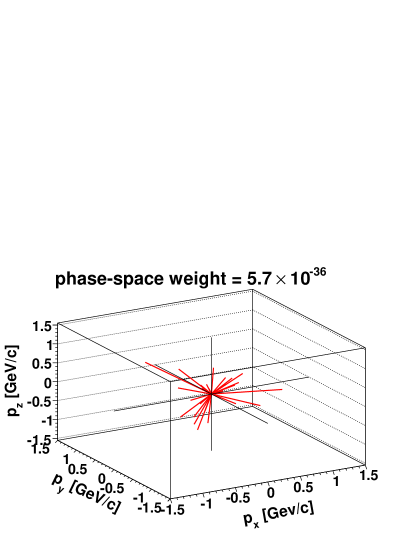
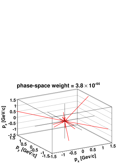
We select (via Monte-Carlo) genbod events according to their weight and run them through identical software as used for experimental analysis. Fortunately, the code is fast, since one must calculate large statistics from which to select. This is because the phase-space weights vary by large factors. As a very extreme case, Figures 1 and 2 show a likely and unlikely event, respectively, for multiplicity $N=30$. As one would expect, the “rounder” event is more likely, though one might be surprised by the factor of a hundred million between the probabilities.

Figure 1: (Color online) A high-probability multiplicity-30 event calculated by genbod . Lines correspond to particle momenta $p_{x},p_{y},p_{z}$.

Figure 2: (Color online) A low-probability multiplicity-30 event calculated by genbod . Lines correspond to particle momenta $p_{x},p_{y},p_{z}$.

III SPHERICAL HARMONIC DECOMPOSITION OF CORRELATION FUNCTIONS

Figure 3: (Color online) 1D projections of 3D correlation function calculated in LCMS frame for multiplicity-9 event calculated by genbod .

Figure 4: (Color online) Correlation function for the same data presented in Fig. 3 is shown at a fixed value of $Q=0.79~{}GeV/c$ (approximately indicated by the shaded region in Fig. 3) as a function of $\phi$ for five bins in $\cos(\theta)$. Curves represent the SHD components of various orders; see text for more details.

Figure 5: (Color online) SHD coefficients for genbod -generated events consisting of 9 pions having average kinetic energy per particle $\bar{K}=0.9$ GeV, as measured in the pair LCMS frame. No kinematic cuts were applied to data. Green squares are $A_{l,m}$’s from the genbod events. Gold inverted triangles are the SHD coefficients of Equation 24 for k=2. Black circles, blue stars and red triangles are SHD coefficients of the first, second and third terms, respectively, of the right side of Equation 25. Open circles are SHD coefficients of the right side of Equation 25.

Measurements of the space-time extent of a particle-emitting source at the femtometer scale is commonly done by analyzing two-particle correlation functions $C\left(\vec{q}\right)$ as a function of the relative momentum $\vec{q}$. Experimentally, $C\left(\vec{q}\right)$ is the ratio of the $\vec{q}$ distribution when both particles are measured in the same event, to the same distribution when the two particles come from different events (c.f. e.g. Lisa:2005dd, , and references therein, for more details). In this Section, we present correlation functions produced in exactly the manner in which experimental ones are formed. genbod -generated events are selected according to the returned event weight.

Ideally, then, any structure remaining in this ratio reflects the correlation between particles in the same event. In the present study, these correlations come from energy and momentum conservation effects.

In this paper we will use the commonly used Bertsch-Pratt (“out-side-long”) decomposition of the relative momentum $\vec{q}$ Pratt:1986cc ; Bertsch:1988db , where $q_{o}$ is parallel to the transverse total momentum of the pair, $q_{l}$ is parallel to the beam direction and $q_{s}$ is perpendicular to those.

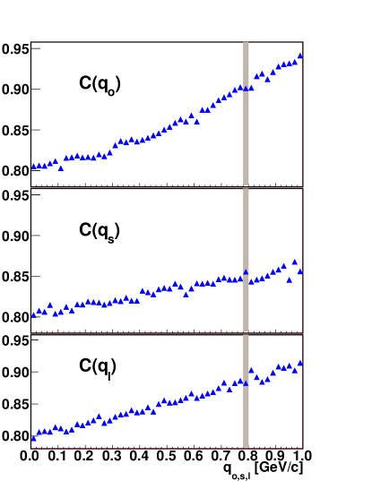
Usually the 3-D correlation functions are presented in 1-D Cartesian projections (or slices) along these axes (e.g. $q_{o}$) with the other q-components (e.g. $q_{s}$ and $q_{l}$) small. Such 1-D slices for genbod calculations are presented on Figure 3. At asymptotically high relative momentum $|\vec{q}|$, femtoscopic contributions to the the correlation function (those described by the Koonin-Pratt equation (discussed in Lisa:2005dd, )) must approach a constant value, usually normalized to unity, independent of the direction of $\vec{q}$. Naturally there are no femtoscopic correlations in these events; correlations induced by the global conservation laws are signaled by the non-unity value of the correlation function. The correlation function depends on the direction of $\vec{q}$ as well as $|\vec{q}|$.

However, one-dimensional projections represent a set of zero measure of the 3-D correlation function and are thus a poor tool for exploring its detailed and potentially important structure. In principle, one could visualize the full structure of the 3-D correlation function via a series of Cartesian projections in $q_{i}$ over different ranges in $q_{j,k}$, where $i\neq j\neq k$. This would, however, constitute a large number of figures, and relevant patterns which cut across projections might not stand out.

By exploiting symmetries in $\vec{q}$-space, the spherical harmonic decomposition (SHD)  becomes a much more efficient representation which uses all of the data to show the shape of the correlation function. Here, the spherical coordinates $\theta$, $\phi$, and $Q=|\vec{q}|$ relate to the Cartesian ones as

$$q_{o}=Q\sin{\theta}\cos{\phi},\qquad q_{s}=Q\sin{\theta}\sin{\phi},\qquad q_{l}=Q\cos{\theta},$$ (3)

and we define harmonic moments $A_{l,m}$’s as

$${\mbox{$A_{l,m}(Q)$}}\equiv\frac{1}{\sqrt{4\pi}}\int d\phi d(\cos\theta)C\left(Q,\theta,\phi\right)Y_{l,m}\left(\theta,\phi\right).$$ (4)

Usually, experimentally measured correlation functions are not continuous functions of $Q$, $\cos\theta$ and $\phi$, but are constructed with bins of finite size. In this case, Equation 4 needs modification to account for finite-bin-size effects. For the experimental practitioner, we discuss one way to deal with this in Appendix C. For the remainder of this manuscript, we will assume these binning effects have been dealt with; i.e. we assume negligible bin size in $\cos\theta$ and $\phi$.

Symmetry constrains the number of relevant components. For femtoscopic analyses of identical particles at midrapidity which integrate over reaction-plane orientation (i.e. almost all analyses to date), only real parts of $A_{l,m}$’s with even values of $l$ and $m$ do not vanish. For the complete list of symmetries of $A_{l,m}$’s, see Appendix B. Further, it is natural to expect that the statistical relevance of high-$l$ components is diminished.

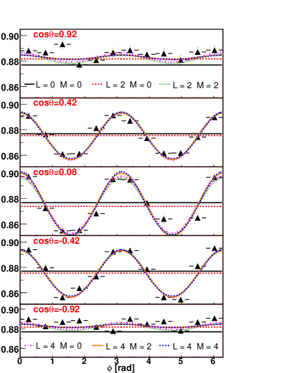
As an example, Fig. 4 shows the calculated correlation function (the same as shown in Fig. 3) for one value of $Q$ as a function of $\cos\theta$ and $\phi$. Also shown are curves representing SHD with increasingly higher order components. In particular, the curves correspond to

$$C_{L,M}(Q,\theta,\phi) \equiv \sqrt{4\pi}\left(\sum_{l=0}^{L-2}\sum_{m=-l}^{l}A_{l,m}(Q)Y^{*}_{l,m}(\theta,\phi)\right.$$ (5)

$$+ \left.\sum_{m=-M}^{M}A_{L,m}(Q)Y^{*}_{L,m}(\theta,\phi)\right).$$

For example, the curve labeled as “L=2 M=0” contains $A_{0,0}$ (the constant term) and $A_{2,0}$ components.

Clearly, for this example, only the first few components are required to represent the structure of the correlation function. While a few higher-$l$ terms may be required in some cases, the number of relevant $A_{l,m}$’s is generically expected to be small. This is from general considerations of smoothness and, for experimental data, statistical issues. Thus, by glancing at only a few one-dimensional plots, one views the entire correlation structure in orthogonal components. The number of plots is usually reduced further by symmetry constraints (c.f. Appendix B).

As an example, the first few $A_{l,m}$’s for the same genbod calculations presented in this section, are plotted as a function of $Q$ in Fig. 5. The odd-$l$ and -$m$ moments (not shown) vanish as required by symmetry (c.f. Appendix B).

IV EMCICS from genbod 

Figure 6: (Color online) SHD coefficients for genbod -generated events consisting of 18 pions having average kinetic energy per particle $\bar{K}=0.9$ GeV, as measured in the pair LCMS frame. No kinematic cuts were applied to data. Green squares are $A_{l,m}$’s from the genbod events. Gold inverted triangles are the SHD coefficients of Equation 24 for k=2. Black circles, blue stars and red triangles are SHD coefficients of the first, second and third terms, respectively, of the right side of Equation 25. Open circles are SHD coefficients of the right side of Equation 25.

Figure 7: (Color online) SHD coefficients for genbod -generated events consisting of 6 pions having average kinetic energy per particle $\bar{K}=0.9$ GeV, as measured in the pair LCMS frame. No kinematic cuts were applied to data. Green squares are $A_{l,m}$’s from the genbod events. Gold inverted triangles are the SHD coefficients of Equation 24 for k=2. Black circles, blue stars and red triangles are SHD coefficients of the first, second and third terms, respectively, of the right side of Equation 25. Open circles are SHD coefficients of the right side of Equation 25.

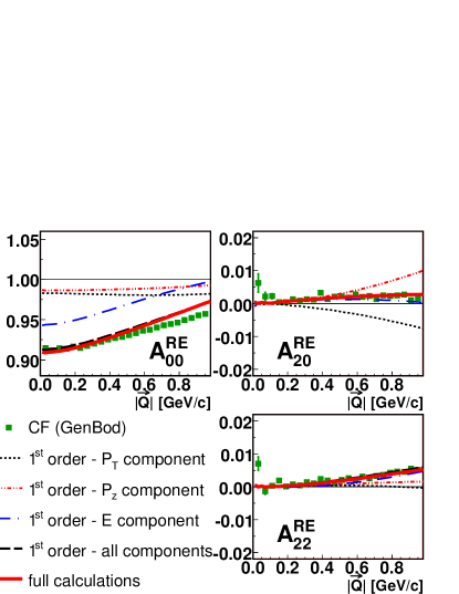
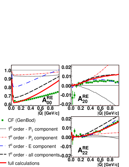
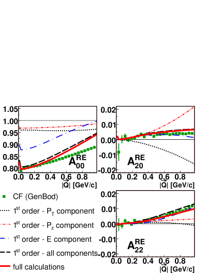
In this Section, we briefly discuss factors which affect the $A_{l,m}$moments, using Figures 5-10. For the present, we focus only on the green squares, labeled “CF (GenBod),” in those Figures.

Figures 5, 6 and 7 show the $A_{l,m}$’s calculated in LCMS frame Lisa:2005dd from genbod events that have the same average kinetic energy per particle ($\bar{K}=0.9$ GeV) but different multiplicity. As expected, the strength of the EMCICs decreases with event multiplicity. Similarly, for a given event multiplicity, one expects larger EMCICs when there is less available energy. As shown in Figures 6 and 8 for multiplicity-18 events, this is indeed the case.

Figure 8: (Color online) SHD coefficients for genbod -generated events consisting of 18 pions having average kinetic energy per particle $\bar{K}=0.5$ GeV, as measured in the pair LCMS frame. No kinematic cuts were applied to data. Green squares are $A_{l,m}$’s from the genbod events. Gold inverted triangles are the SHD coefficients of Equation 24 for k=2. Black circles, blue stars and red triangles are SHD coefficients of the first, second and third terms, respectively, of the right side of Equation 25. Open circles are SHD coefficients of the right side of Equation 25.

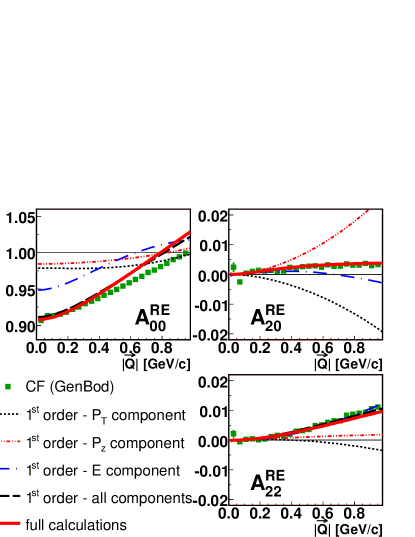
Since the definition of the “out,” “side” and “long” directions– and thus the angles $\theta$ and $\phi$– depend on the frame of measurement, one expects the spherical harmonic coefficients $A_{l,m}$to depend on reference frame. This is shown in Figures 6 and 9 for correlations measured in LCMS and pair CMS frames.

Figure 9: (Color online) SHD coefficients for genbod -generated events consisting of 18 pions having average kinetic energy per particle $\bar{K}=0.9$ GeV, as measured in the pair CMS frame. No kinematic cuts were applied to data. Green squares are $A_{l,m}$’s from the genbod events. Gold inverted triangles are the SHD coefficients of Equation 24 for k=2. Black circles, blue stars and red triangles are SHD coefficients of the first, second and third terms, respectively, of the right side of Equation 25. Open circles are SHD coefficients of the right side of Equation 25.

Figure 10: (Color online) SHD coefficients for genbod -generated events consisting of 18 pions having average kinetic energy per particle $\bar{K}=0.9$ GeV, as measured in the pair CMS frame. Only particles with $|\eta|<0.5$ used in the correlation function. Green squares are $A_{l,m}$’s from the genbod events. Gold inverted triangles are the SHD coefficients of Equation 24 for k=2. Black circles, blue stars and red triangles are SHD coefficients of the first, second and third terms, respectively, of the right side of Equation 25. Open circles are SHD coefficients of the right side of Equation 25.

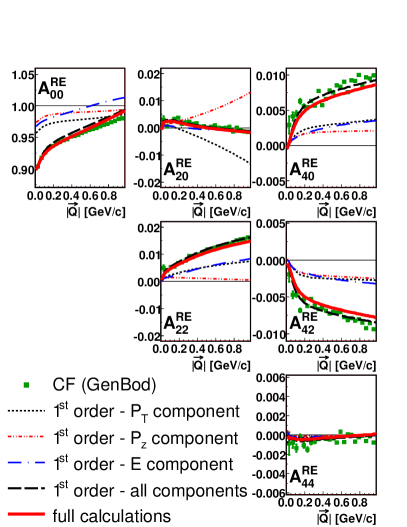
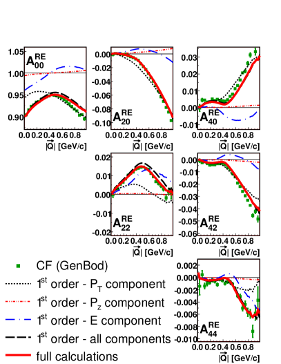
Less intuitive is the observation that the correlation strength depends also on kinematic cuts. Figures 9 and 10 show the $A_{l,m}$’s calculated by genbod for 18-pion events without and with a selection of $|\eta|<0.5$, respectively. (Note that this cut applies to the pions which are used in the analysis, not to the set of particles for which energy and momentum is conserved; energy and momentum is always conserved for the full event.)

Finally, we note two important and generic effects. Firstly, EMCICs are present at all values of $|\vec{Q}|$, reminding us that we cannot (responsibly) ignore these effects in a femtoscopic analysis. Secondly, in Figures 9 and 10, we have included $A_{l,m}$components up to $l=4$. Typically, $|A_{l+2,m}/{\mbox{$A_{l,m}$}}|\sim 0.1$, another reminder that characterization of the 3-dimensional correlation function requires only a few harmonic components.

V ANALYTIC CALCULATION OF EMCICs

Even if EMCIC effects generated by genbod “resemble” the experimental data, it is likely unwise to use genbod itself to correct the data for several reasons. Firstly, there is strong sensitivity to the (not completely measured) number and species-mix of all particles emitted in the event, including neutrinos and possible magnetic monopoles (or, less exotically, particles escaping detector acceptance). Secondly, there is strong sensitivity to the energy “available” in the event; it is not obvious that this is $\sqrt{s_{NN}}$ of the collision. Thirdly, EMCIC effects depend on the individual momenta $\vec{p}_{1}$ and $\vec{p}_{2}$ of the particles entering the correlation function. This will depend on acceptance, efficiency, kinematic cuts and, to a degree, the underlying single-particle phase-space. (While correlation functions are insensitive to the single-particle phase-space, the correlations which they measure may, in fact, depend on this phase-space, due to physical effects.)

Thus, one would like to calculate EMCICs, based on the data itself. In this Section, we begin by following arguments similar to those in Refs Danielewicz:1987in ; Borghini:2000cm ; Borghini:2003ur to obtain correction factors which implement EMCICs onto multi-particle distributions. In the course of the calculation, we make some simplifying approximations. The derived expressions are then tested for accuracy against the numerical genbod simulations. Finally, the expressions are used to extract an “experimentalist’s formula” discussed in the next Section.

V.1 Restricted phase-space corrections

Danielewicz Danielewicz:1987in , and later Borghini, Dinh and Ollitrault Borghini:2000cm , considered EMCIC-type effects on two-particle azimuthal correlations (quantified by $v_{2}$ and often used as a measure of elliptic flow Ollitrault:1992bk ). They focused mostly on transverse momentum ($\vec{P}_{T}$) conservation only, but Borghini later Borghini:2003ur generalized to the case of an arbitrary number $D$ of independent (orthogonal) spatial dimensions and recently considered momentum conservation effects on three-particle analyses of jet-like behavior Borghini:2006yk .

As we shall see below, for correlation functions used in femtoscopy, the conservation of energy generates effects of similar magnitude as those due to conservation of (three-)momentum. We deal only with on-shell particles, for which energy cannot be treated as independent of the momentum (as, say, $p_{x}$ would be largely independent of $p_{y}$). Thus, unlike the above-mentioned works, we will explicitly begin with the more general multivariate central limit theorem.

We start with the case of interest– $D=3$ spatial dimensions– and conserve 3-momentum $\vec{p}$. We implement energy conservation and on-shell constraints a bit later.

We define 

$$f\left(\vec{p}_{i}\right)\equiv\frac{d^{3}N}{d\vec{p}^{3}_{i}}$$ (6)

as the single-particle momentum distribution unaffected by EMCICs. This may be considered the unmeasured “parent” distribution. Then, the $k-$particle distribution ($k$ less than the total multiplicity $N$) including EMCICs is

$${f}_{c}\left(\vec{p}_{1},...,\vec{p}_{k}\right)=\left(\prod_{i=1}^{k}{f}(\vec{p}_{i})\right)\times\qquad\qquad\qquad\qquad$$

$$\frac{\int\left(\prod_{j=k+1}^{N}d^{3}\vec{p}_{j}{f}\left(\vec{p}_{j}\right)\right)\delta^{3}\left(\sum_{i=1}^{N}\vec{p}_{i}\right)}{\int\left(\prod_{j=1}^{N}d^{3}\vec{p}_{j}{f}\left(\vec{p}_{j}\right)\right)\delta^{3}\left(\sum_{i=1}^{N}\vec{p}_{i}\right)}.$$ (7)

Note the difference between numerator and denominator in the starting value of the index $j$ on the product.

We implement total energy conservation $\sum E_{i}=\sqrt{s}$, by replacing $\delta^{3}\left(\sum_{i=1}^{N}\vec{p}_{i}\right)\rightarrow\delta^{4}\left(\sum_{i=1}^{N}p_{i}-P\right)$ in Equation V.1. Here, $P=\left(\sqrt{s},\vec{0}\right)$ is the total energy-momentum of the event, and $p_{0,i}=E_{i}=\sqrt{\vec{p}_{i}^{2}+m_{i}^{2}}$ is the energy of the on-shell particle.

We denote Lorentz-invariant distributions as

$$\tilde{f}(p_{i})\equiv 2E_{i}\frac{d^{3}N}{d\vec{p}_{i}^{3}}=2E_{i}f(p_{i})$$ (8)

and rewrite Equation V.1 as

$$\tilde{f}_{c}\left(p_{1},...,p_{k}\right)=\left(\prod_{i=1}^{k}\tilde{f}(p_{i})\right)\times\qquad\qquad\qquad\qquad$$ (9)

$$\frac{\int\left(\prod_{j=k+1}^{N}\frac{d^{3}\vec{p}_{j}}{E_{j}}\tilde{f}\left(\vec{p}_{j}\right)\right)\delta^{4}\left(\sum_{i=1}^{N}p_{i}-P\right)}{\int\left(\prod_{j=1}^{N}\frac{d^{3}\vec{p}_{j}}{E_{j}}\tilde{f}\left(\vec{p}_{j}\right)\right)\delta^{4}\left(\sum_{i=1}^{N}p_{i}-P\right)}$$

$$= \left(\prod_{i=1}^{k}\tilde{f}(p_{i})\right)\times\qquad\qquad\qquad\qquad$$

$$\frac{\int\left(\prod_{j=k+1}^{N}d^{4}p_{j}\delta\left(p^{2}_{j}-m^{2}_{j}\right)\tilde{f}\left(p_{j}\right)\right)\delta^{4}\left(\sum_{i=1}^{N}p_{i}-P\right)}{\int\left(\prod_{j=1}^{N}d^{4}p_{j}\delta\left(p^{2}_{j}-m^{2}_{j}\right)\tilde{f}\left(p_{j}\right)\right)\delta^{4}\left(\sum_{i=1}^{N}p_{i}-P\right)}$$

$$= \left(\prod_{i=1}^{k}\tilde{f}(p_{i})\right)\times\qquad\qquad\qquad\qquad$$

$$\frac{\int\left(\prod_{j=k+1}^{N}d^{4}p_{j}g\left(p_{j}\right)\right)\delta^{4}\left(\sum_{i=1}^{N}p_{i}-P\right)}{\int\left(\prod_{j=1}^{N}d^{4}p_{j}g\left(p_{j}\right)\right)\delta^{4}\left(\sum_{i=1}^{N}p_{i}-P\right)}.$$

Thus, we arrive at an integral over four independent variables, in which the integrand function $g(p)$ is “highly peaked” and with strong correlations in the 4-d $p-$space.

According to Equation 9, the $k$-body momentum distribution, including EMCICs, is the $k$-body distribution not affected by EMCICs– i.e. just an uncorrelated product of single-particle distributions– multiplied by a “correction factor” which enforces the EMCIC. The numerator of this factor counts the number of configurations in which the remaining $N-k$ on-shell particles conspire to conserve total energy and momentum, and the denominator normalizes the distribution.

V.2 Application of the Central Limit Theorem

To arrive at a useful result, we argue along lines similar to those of Danielewicz:1987in ; Borghini:2000cm ; Borghini:2003ur . The distribution of a large number $M$ of uncorrelated momenta $W=\sum_{i=1}^{M}p_{i}$ is, by the Central Limit Theorem, a multivariate normal distribution

$$F_{M}\left(W\right) \equiv \int\left(\prod_{i=1}^{M}d^{4}p_{i}g(p_{i})\right)\delta^{4}\left(\sum_{i=1}^{M}p_{i}-W\right)$$

$$= \sqrt{\frac{|B|}{\left(2\pi\right)^{4}}}\times$$

$$\exp\left(-\frac{1}{2}\left(W^{\mu}-\langle P^{\mu}\rangle\right)B_{\mu\nu}\left(W^{\nu}-\langle P^{\nu}\rangle\right)\right).$$

Here, the average of the sum of 4-momenta is simply related to the single-particle average of the 4-momenta as

$$\langle P^{\mu}\rangle = \sum_{i=1}^{M}\langle p_{i}^{\mu}\rangle=M\langle p_{i}^{\mu}\rangle,$$ (11)

where

$$\langle p^{n}_{\mu}\rangle\equiv\frac{\int d^{4}pg(p)\cdot p_{\mu}^{n}}{\int d^{4}pg(p)},$$

$$\langle p_{\mu}p_{\nu}\rangle\equiv\frac{\int d^{4}pg(p)p_{\mu}p_{\nu}}{\int d^{4}pg(p)}.$$ (12)

Finally, in Equation V.2, $|B|$ denotes the determinant of the matrix $B$. Up to a factor of $M$, $B$ is the inverse of the covariance matrix of the distribution $g(p)$:

$$B_{\mu\nu} = \frac{1}{M}b_{\mu\nu},$$ (13)

$$\left(b^{-1}\right)_{\mu\nu} = \langle p_{\mu}p_{\nu}\rangle-\langle p_{\mu}\rangle\langle p_{\nu}\rangle.$$ (14)

We can now apply the CLT by recognizing the integral in the numerator in Equation 9 as the distribution of $N-k$ momenta $\sum_{j=k+1}^{N}p_{j}=P-\sum_{j=1}^{k}p_{j}$ so that for “large enough” $N-k$, we find

$$\tilde{f}_{c}\left(p_{1},...,p_{k}\right)=\left(\prod_{i=1}^{k}\tilde{f}(p_{i})\right)\frac{F_{N-k}\Big{(}P-\sum_{i=1}^{k}p_{i}\Big{)}}{F_{N}(P)}$$

$$=\left(\prod_{i=1}^{k}\tilde{f}(p_{i})\right)\cdot\left(\frac{N}{N-k}\right)^{2}\times$$ (15)

$$\exp\left[-\left(\sum_{i=1}^{k}\left(p_{i}^{\mu}-\langle p^{\mu}\rangle\right)\right)\frac{b_{\mu\nu}}{2\left(N-k\right)}\left(\sum_{i=1}^{k}\left(p_{i}^{\nu}-\langle p^{\nu}\rangle\right)\right)\right].$$

It is appropriate at this point to repeat the two approximations we have employed up to now. The first assumption, always important in using the CLT, is that $N-k$ is sufficiently large; recall that $N$ is the total multiplicity and $k$ is the order of the correlation being calculated ($k=2$ for two-particle correlations). Secondly, we have implicitly assumed that all particles in the system are governed by the same single-particle distribution $g(p)$. Strictly speaking, then, the system must consist of particles all of the same mass, and if there are several species with the same mass (say, $\pi^{-}$ and $\pi^{+}$), they must furthermore have the same momentum distribution. This is at best an approximation for hadron or ion collisions, in which other particles contribute to the pion-dominated final state.

V.3 Observable EMCIC effects

Even the single-particle momentum distribution is affected by EMCICs:

$$\tilde{f}_{c}\left(p_{i}\right) = \tilde{f}\left(p_{i}\right)\cdot\left(\frac{N}{N-1}\right)^{2}\times$$ (16)

$$\exp\left[-\left(p^{\mu}-\langle p^{\mu}\rangle\right)\frac{b_{\mu\nu}}{2\left(N-k\right)}\left(p^{\nu}-\langle p^{\nu}\rangle\right)\right]$$

The product of such a single particle distribution forms the denominator of the $k$-particle correlation function

$$C\left(p_{1},...,p_{k}\right)\equiv\frac{\tilde{f}_{c}\left(p_{1},...,p_{k}\right)}{\tilde{f}_{c}\left(p_{1}\right)\cdots\tilde{f}_{c}\left(p_{k}\right)}=\frac{\left(\frac{N}{N-k}\right)^{2}}{\left(\frac{N}{N-1}\right)^{2k}}\times\qquad$$ (17)

$$\frac{\exp\left[\frac{-1}{2(N-k)}\sum_{i,j=1}^{k}\left(p_{i}^{\mu}-\langle p^{\mu}\rangle\right)b_{\mu\nu}\left(p_{j}^{\nu}-\langle p^{\nu}\rangle\right)\right]}{\exp\left[\frac{-1}{2(N-1)}\sum_{i=1}^{k}\left(p_{i}^{\mu}-\langle p^{\mu}\rangle\right)b_{\mu\nu}\left(p_{i}^{\nu}-\langle p^{\nu}\rangle\right)\right]}$$

In this paper we concentrate on correlation functions in $q_{out},q_{side}$ and $q_{long}$, as is done in femtoscopic studies. However, the two-particle correlation function in relative azimuthal angle, which probes elliptic flow, may also contain EMCIC contributions through Equation 17. These effects turn out to be small and are discussed in Appendix A.

To first order in $1/N$, the two-particle correlation function becomes

$$C(p_{1},p_{2})=1-\frac{1}{N}\left(p_{1}^{\mu}-\langle p^{\mu}\rangle\right)b_{\mu\nu}\left(p_{2}^{\nu}-\langle p^{\nu}\rangle\right).$$ (18)

The multivariate CLT used in Section V.2 accounts for correlations between vector components via the covariance matrix $b^{-1}$ (Eq. 14) which has, in general, 10 nonvanishing elements. The average vector $P$ (Eq. 11) has in general 4 nonvanishing elements. We now reduce these numbers significantly by considering the specific case of our interest.

Firstly, we choose to work in the global center-of-momentum frame, so that

$$\langle p^{\mu}\rangle=\delta_{\mu,0}\langle E\rangle$$ (19)

As for the correlations, we are interested in signals generated by EMCICs alone, not, for example, dynamical correlations due to flow. Neglecting elliptic flow (azimuthal anisotropies in the parent distribution Ollitrault:1992bk ; Poskanzer:1998yz ) implies

$$\left(b^{-1}\right)_{1,2}=\langle p_{x}p_{y}\rangle=0.$$ (20)

The same approach was adopted in earlier work Danielewicz:1987in ; Borghini:2000cm ; Borghini:2006yk . Similarly, we assume no dynamical correlations due to directed flow Poskanzer:1998yz , implying

$$\left(b^{-1}\right)_{1,3}=\left(b^{-1}\right)_{2,3}=0.$$ (21)

The on-shell constraint generates an unavoidable dependence between energy and 3-momentum components. However, in the CLT limit, only the second moment (covariance) comes into play, and this vanishes. For $i\neq 0$,

$$\left(b^{-1}\right)_{0,i}=\langle Ep_{i}\rangle-\langle E\rangle\langle p_{i}\rangle=\langle Ep_{i}\rangle$$ (22)

$$=\frac{\int dE\int d^{3}\vec{p}\cdot Eg\left(p\right)\cdot p_{i}}{\int dE\int d^{3}\vec{p}\cdot g\left(p\right)}=0.$$

In the last step, we recognize that $p_{i}$ is an odd function of momentum, whereas $E$ and $g$ are even.

In this scenario of interest, then, $b$ is diagonal, and Equations 16 becomes

$$\tilde{f}_{c}\left(p_{i}\right)=\tilde{f}\left(p_{i}\right)\cdot\left(\frac{N}{N-1}\right)^{2}\times$$ (23)

$$\exp\left[-\frac{1}{2(N-1)}\left(\frac{p^{2}_{i,x}}{\langle p_{x}^{2}\rangle}+\frac{p^{2}_{i,y}}{\langle p_{y}^{2}\rangle}+\frac{p^{2}_{i,z}}{\langle p_{z}^{2}\rangle}+\frac{\left(E_{i}-\langle E\rangle\right)^{2}}{\langle E^{2}\rangle-\langle E\rangle^{2}}\right)\right].$$

Similarly, Equation 17 becomes

$$C\left(p_{1},...,p_{k}\right)\equiv\frac{\tilde{f}_{c}\left(p_{1},...,p_{k}\right)}{\tilde{f}_{c}\left(p_{1}\right)\cdots\tilde{f}_{c}\left(p_{k}\right)}=\frac{\left(\frac{N}{N-k}\right)^{2}}{\left(\frac{N}{N-1}\right)^{2k}}\times\qquad$$ (24)

$$\frac{\exp\left[\frac{-1}{2(N-k)}\left\{\sum_{\mu=1}^{3}\left(\frac{\left(\sum_{i=1}^{k}p_{i,\mu}^{2}\right)^{2}}{\langle p_{\mu}^{2}\rangle}\right)+\frac{\left(\sum_{1}^{k}\left(E_{i}-\langle E\rangle\right)\right)^{2}}{\langle E^{2}\rangle-\langle E\rangle^{2}}\right\}\right]}{\exp\left[\frac{-1}{2(N-1)}\sum^{k}_{i=1}\left\{\sum_{\mu=1}^{3}\frac{p_{i,\mu}^{2}}{\langle p_{\mu}^{2}\rangle}+\frac{\left(E_{i}-\langle E\rangle\right)^{2}}{\langle E^{2}\rangle-\langle E\rangle^{2}}\right\}\right]}$$

and Equation 18 becomes

$$C(p_{1},p_{2})=1-$$ (25)

$$\frac{1}{N}\left(2\frac{\vec{p}_{1,T}\cdot\vec{p}_{2,T}}{\langle p_{T}^{2}\rangle}+\frac{p_{1,z}\cdot p_{2,z}}{\langle p_{z}^{2}\rangle}+\frac{\left(E_{1}-\langle E\rangle\right)\left(E_{2}-\langle E\rangle\right)}{\langle E^{2}\rangle-\langle E\rangle^{2}}\right),$$

where we have taken $\langle p_{x}^{2}\rangle=\langle p_{y}^{2}\rangle=\langle p^{2}_{T}\rangle/2$ in the azimuthally-symmetric case of interest. In what follows and in Figures 5-10, we shall refer to the first, second, and third terms within the parentheses of Equation 25 as the “$p_{T}$” “$p_{z}$” and “$E$” components, respectively.

If we somehow know $N$, $\langle p_{T}^{2}\rangle$, $\langle p_{z}^{2}\rangle$, $\langle E^{2}\rangle$ and $\langle E\rangle$, we can calculate EMCICs using Equation 24. (See, however, the discussion at the start of the next Section.) Better yet, if $N$ is large enough, then we can use Equation 25. This is what is done in Figures 5-10. The open circles and orange inverted triangles represent the results of Equation 24 and Equation 25, respectively. The black circles, blue stars, and red triangles show the individual components of Equation 25; this decomposition will be relevant when we discuss the “experimentalist’s formula” in the next Section.

Figures 5-10 make clear that each of the three terms in Equation 25 produces non-trivial behavior of the $A_{l,m}$’s. Also clear is the importance of not neglecting the energy term. We find also that the $p_{z}$ term affects $A_{2,2}$; this may be surprising since $A_{2,2}$ quantifies the behavior of the correlation function in the “out-side” plane, while $\hat{z}$ is the “long” direction in the Bertsch-Pratt system. Clearly, EMCICs projected onto a 2-particle space are non-trivial objects.

The first-order expansion (Equation 25) agrees well with the full expression (Equation 24) well for $N\gtrsim 10$. Such multiplicities are relevant for $p+p$ measurements at RHIC (recalling that $N$ includes all particles, even unmeasured ones). We see also that the analytic calculations (open circles and inverted triangles) approximate the results of the genbod simulation (green squares), especially as the multiplicity and total energy of the event increases; increasing agreement for large $N$ and $E_{tot}$ is expected, given the approximations leading to our analytic expressions. We observe also that the analytically-calculated expressions respond identically to the kinematic cuts as does the simulation (c.f. Figures 9 and  10).

Finally, the analytic calculations never reproduce exactly the simulations; we discuss this further in the next Section.

VI AN EXPERIMENTALIST’S FORMULA

Even for large $N$ and energy, the calculations do not exactly reproduce the EMCIC effects in the simulation. One reason for this may be found, in fact, in the definition of the average values (e.g. $\langle p_{z}^{2}\rangle$) themselves. In Equation V.2, average quantities are calculated using the distribution $\tilde{f}(p)$, which is not affected by EMCICs. Naturally, the only measurable distribution available to the experimentalist (even when genbod simulations serve as the “experiment”) is $\tilde{f}_{c}(p)$.

Thus, it appears the experimentalist cannot plug her data into the equations V.2 and 25 to fully calculate EMCICs. However, such an ambition would have been hopeless anyhow. After all, even the total multiplicity $N$ (again, including photons etc) is rarely fully measured, and in principle $N$ is a number of “primary” particles, a murky concept in itself.

To the practicing femtoscopist, there is a natural solution. Having at hand (1) educated guesses for the quantities $N$, $\langle E^{2}\rangle$ etc, and (2) a physically-motivated functional form which connects these quantities to the correlations, one may perform a fit. Let us rewrite Equation 25 as

$$C\left(p_{1},p_{2}\right)=1-M_{1}\cdot\overline{\left\{\vec{p}_{1,T}\cdot\vec{p}_{2,T}\right\}}-M_{2}\cdot\overline{\left\{p_{1,z}\cdot p_{2,z}\right\}}\quad$$ (26)

$$-M_{3}\cdot\overline{\left\{E_{1}\cdot E_{2}\right\}}+M_{4}\cdot\overline{\left\{E_{1}+E_{2}\right\}}-\frac{M_{4}^{2}}{M_{3}},\qquad$$

where

$$M_{1}\equiv\frac{2}{N\langle p_{T}^{2}\rangle}\quad,\quad M_{2}\equiv\frac{1}{N\langle p_{z}^{2}\rangle}\qquad\qquad\qquad$$

$$M_{3}\equiv\frac{1}{N\left(\langle E^{2}\rangle-\langle E\rangle^{2}\right)}\quad,\quad M_{4}\equiv\frac{\langle E\rangle}{N\left(\langle E^{2}\rangle-\langle E\rangle^{2}\right)}.$$ (27)

The notation $\overline{\left\{X\right\}}$ in Equation 26 highlights the fact that $X$ is a two-particle quantity which depends on $p_{1}$ and $p_{2}$ (or $\vec{q}$, etc). From a practical point of view, $X$ will be averaged over the same $\vec{q}$ bins as used for the correlation function. For infinitesimally narrow $q$-bins, $\overline{\left\{X\right\}}=X$. The binned functions $\overline{\left\{X\right\}}$ then automatically reflect the same event and particle selection as the correlation function. This involves nothing more than adding four more histograms to the several already being constructed by the experimentalist as she processes pairs in the data.

Here, we should emphasize that, in Equation 26, $\vec{p_{1}}$, $E_{1}$, $\vec{p_{2}}$, and $E_{2}$ should be calculated in the collision center-of-momentum (CCM) frame. The reason is that Equation 9 (hence Eqs. V.2-VI) assumes some fixed total energy and momentum to be conserved. The event’s total energy and momentum (hence $\langle E\rangle$, $\langle\vec{p}\rangle$, etc appearing in Eqs. V.2-VI) are fixed quantities in any given frame. In a pair-dependent frame (e.g. LCMS), the total energy and momentum of the event will fluctuate, pair-by-pair. Thus, while the correlation function may be binned in whatever frame one chooses, the momenta $p^{\mu}_{i}$ on the right side of Eqs. 9-VI must be calculated in a pair-independent frame. In fact, starting with Equation 19, we have chosen the CCM, for simplicity.

The parameters $M_{i}$ defined in Equation VI, on the other hand, are global and independent of $p_{1}$ and $p_{2}$. It is these which we will use as fit parameters. The task is then fast and straightforward; the EMCIC part of the correlation function $C(\vec{q})$ is simply a weighted sum of four functions. Indeed, one may calculate coefficients as in Equation 4 for the four new functions. For example

$$A_{l,m}^{p_{Z}}\left(Q\right)\equiv\sum_{{\rm bins}\thinspace i}\overline{\left\{p_{1,z}\cdot p_{2,z}\right\}}\left(Q,\cos\theta_{i},\phi_{i}\right)\cdot Y_{l,m}\left(\cos\theta_{i},\phi_{i}\right),$$ (28)

etc. Then, thanks to the linearity of Equation 26 and the orthonormality of $Y_{l,m}$’s, the measured $A_{l,m}$’s themselves are similarly just weighted sums of harmonics

$${\mbox{$A_{l,m}(Q)$}}=\delta_{l,0}\cdot\left(1-M_{4}^{2}/M_{3}\right)-M_{1}\cdot A_{l,m}^{p_{T}}\left(Q\right)\qquad$$ (29)

$$-M_{2}\cdot A_{l,m}^{p_{Z}}\left(Q\right)-M_{3}\cdot A_{l,m}^{(E\cdot E)}\left(Q\right)+M_{4}\cdot A_{l,m}^{(E+E)}\left(Q\right).$$

Treating Equation 29 as a fit, we have a few (say six, for $l\leq 4$) one-dimensional functions to fit with four adjustable weights. The number of degrees of freedom in this four-parameter fit remains high: $\sim 300$, for six $A_{l,m}$’s, each with 50 bins in $|Q|$.

Figure 11: (Color online) Green inverted triangles show the $\pi^{-}-\pi^{-}$ correlation function, in the pair rest frame, from 18-pion genbod -generated events. The black curve is a result of a fit with the “experimentalist’s formula” from Equation 29. Other curves represent the three component terms of the fit: $M_{1}\cdot A^{p_{T}}_{l,m}(Q)$ in the brown dotted line; $M_{2}\cdot A^{p_{Z}}_{l,m}(Q)$ in the blue dashed line; $M_{3}\cdot A^{E\cdot E}_{l,m}(Q)+M_{4}\cdot A^{E+E}_{l,m}(Q)$ in the red dash-dot line. See text for details.

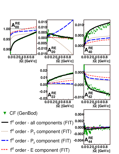
An example is shown in Figure 11, where genbod -calculated correlation functions are fitted with the form of Equation 29. Not surprisingly, the minimization procedure returned fit parameters $M_{i}$ very close to the values calculated via Equation VI. However, exact agreement between the “best” parameter values returned by the fit, and those from Equation VI is not expected. This is because the large-$N$ approximation is only approximately valid and due to the fact that $\tilde{f}(p)\neq\tilde{f}_{c}(p)$, as discussed previously. Treating the $M_{i}$ as adjustable parameters leads to a slightly different weighting of the terms, and a slightly better fit to the data.

Our original goal was not to understand EMCICs per se, but to extract the femtoscopic information from measured two-particle correlations. Assuming that the only non-femtoscopic correlations are EMCICs, one may simply add the femtoscopic terms $\Phi_{\rm femto}(p_{1},p_{2})$ to the fitting function in Equation 26 or 29.

$$C\left(p_{1},p_{2}\right) = \Phi_{\rm femto}(p_{1},p_{2})\times$$

$$\Big{(} 1-M_{1}\cdot\overline{\left\{\vec{p}_{1,T}\cdot\vec{p}_{2,T}\right\}}-M_{2}\cdot\overline{\left\{p_{1,z}\cdot p_{2,z}\right\}}$$

$$- M_{3}\cdot\overline{\left\{E_{1}\cdot E_{2}\right\}}+M_{4}\cdot\overline{\left\{E_{1}+E_{2}\right\}}-\frac{M_{4}^{2}}{M_{3}}\Big{)}.$$

Common femtoscopic fitting functions (e.g. Gaussian in the out-side-long space) usually contain $\sim 5$ parameters (e.g. $N$, $\lambda$, $R_{i}$, $i=o,s,l$). In the imaging technique Brown:1997ku , one assumes the separation distribution is described by a sum of splines, rather than a Gaussian; here, too, there are usually 4-5 fit parameters (spline weights). So, by including EMCIC effects, we have roughly doubled the number of fit parameters, relative to a “traditional” fit which ignores them. This is a non-trivial increase in analysis complexity. However, we keep in mind two points.

Firstly, the increased effort is simply necessary. EMCICs (and possibly other important non-femtoscopic correlations) are present and increasingly relevant at low multiplicity. One option is to ignore them, as has sometimes been done in early high-energy experiments. However, with the new high-quality data and desire for detailed understanding at RHIC, ignoring obvious features such as those presented in Chajecki:2005zw is clearly unacceptable. Perhaps a slightly better option is to invent an ad-hoc functional form Agababyan:1996rg without a strong real physical basis. We hope that the results here present a relatively painless and more reasonable, third option.

Secondly, while the non-femtoscopic EMCICs are not confined to the large-$Q$ region (an important point!), the femtoscopic correlations are confined to the small-$Q$ region. Therefore, one hopes that the addition of four new parameters to the fit of the correlation function will not render the fit overly unwieldy. While we cannot expect complete block-diagonalization of the fit covariance matrix, one hopes that the $M_{i}$ are determined well enough at high $Q$ that the femtoscopic fit parameters can be extracted at low $Q$.

VII Non-identical particle correlations

For at least two reasons, it is important to turn attention to correlations between non-identical particles.

First, it is natural to ask whether one can use other particle combinations to “correct” for effects of EMCICs in, say, identical-pion correlation functions. After all, EMCICs are induced by global constraints on the entire event, not a specific particle species. For example, various experiments have explored using $(\pi^{+},\pi^{-})$ correlations to account for EMCICs in $(\pi^{+},\pi^{+})$ correlation functions Avery:1985qb ; collaboration:2007he ; Chekanov:2003gf .

Second, it is also important to know whether EMCICs could cloud the interpretation of correlations between non-identical particles. It is increasingly common to study asymmetries in the correlation functions of, say $\pi-K$ pairs Adams:2003qa , interpreting such as a “shift” in the average point of emission between the two particles Lednicky:1995vk . In the spherical harmonic decomposition, such shifts appear in the $l=1$ moments (c.f. Appendix B). We will find that EMCICs can indeed generate an asymmetry which might naively be considered proof of a femtoscopic shift.

Here we discuss two effects– one immediately obvious and one more subtle– which are relevant for the above issues. The discussion is broken into three parts. Neglecting EMCICs and any other source of correlation at first, we briefly show the effects of two common resonances on correlations between oppositely-charged pions in a toy model. Thus calibrated, we use the more realistic and complex pythia model to illustrate a non-trivial interplay between EMCICs and the resonances, which can mock up a femtoscopic asymmetry signal. Finally, we return to a toy model– now with non-identical particles and EMCICs, but without resonances or the several other sources of correlation present in pythia – to make clear the mechanism behind the special effects EMCICs have on non-identical particle correlations.

VII.1 Effect of resonances

First we consider the effect of resonances. To focus on effects other than global EMCICs we use a toy model in which only ten identical resonances per event are generated and no other particles. The momentum of each resonance is generated from a thermal distribution; energy and momentum are conserved for each decay separately, but not globally for the whole event.

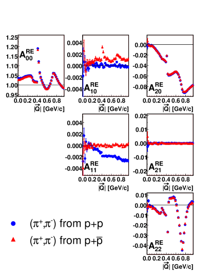
Figure 12 shows the spherical harmonic moments of $(\pi^{+},\pi^{-})$ correlation functions for events including $\omega$ (blue squares) and $\rho$ resonances (red triangles).

Figure 12: (Color online) $(\pi^{+},\pi^{-})$ correlation functions calculated in the LCMS frame for events including $\omega$ (blue squares) and $\rho$ (red triangles) resonances .

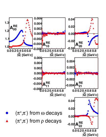
As seen, even without considering EMCICs, the correlations among particles coming from resonance decays produce non-trivial structure. In this case, one cannot simply divide $(\pi^{+},\pi^{+})$ correlation function by $(\pi^{+},\pi^{-})$ to “remove” EMCICs.

Figure 13: (Color online) SHD moments of $(\pi^{+},\pi^{-})$ correlation function from $p+p$ and $p+\bar{p}$ collisions at 200 GeV calculated from pythia events.

VII.2 Entrance channel asymmetries

In addition to the correlation between daughters of resonance decays (c.f. Fig. 12), there is a more subtle effect to consider. This happens when the two particles have different inclusive momentum distributions and energy and momentum are globally conserved. Under these conditions non-identical particle correlations exhibit structure absent in identical particle correlations.

Figure 13 shows pythia  Sjostrand:2000wi calculations of $(\pi^{+},\pi^{-})$ correlations for $p+p$ and $p+\bar{p}$ collisions at 200 GeV. In addition to obvious correlations between daughters of resonance decays ($K_{s}^{0}$, $\omega$, $\rho$), we see additional structure. We focus on the structure in the $l=1$ moments. In general, such moments need not vanish for correlations of non-identical particles, as discussed in Appendix B.

Correlations between sibling daughters of $\rho$ and $\omega$ resonance decay do not generate $l=1$ moments, as seen in Section VII.1. However, pions which are daughters of these decays will in general have a different single-particle momentum distribution than pions from other sources in the event. If the fraction of pions from resonance decay, as a function of pion momentum, is different for $\pi^{+}$ and $\pi^{-}$, then the single-particle distributions of positive and negative pions will be different. We argue below that it is this difference in single-particle distributions which is the key to the non-vanishing $l=1$ moments; that this difference may arise from resonances in the case at hand is irrelevant.

In the $p+\bar{p}$ collisions, the fraction of $\pi^{+}$ coming from any given source (e.g. $\rho$-decay) must be identical to that of $\pi^{-}$, for a given value of $p_{T}$. Thus the $p_{T}$ distribution of $\pi^{-}$ must be identical to that of $\pi^{+}$. However, the rapidity distributions will be mirror images of each other. Thus, any asymmetry in $\pi^{-}-\pi^{+}$ correlations from $p+\bar{p}$ collisions will be associated with $q_{\rm long}$, and will appear in $A_{1,0}$, as seen in Figure 13. Similarly, the vanishing (non-vanishing) moment $A_{1,0}$ ($A_{1,1}$) for $p+p$ collisions reflects the fact the single-particle distributions will show no asymmetry in rapidity, but may differ as a function of $p_{T}$.

Since single-particle distributions divide out of a correlation function, a difference between $\pi^{+}$ and $\pi^{-}$ momentum distributions, by itself, cannot generate a signal in $A_{l,m}$’s. Rather, a global correlation, coupled with this difference, generates the signal. We discuss this further below.

VII.3 A simpler case

In Section VII.2, we argued that the small difference in single-particle momentum distributions between positive and negative pions produced by pythia , coupled with global conservation laws, generated non-trivial EMCICs in the non-identical particle correlations. However, pythia contains many non-EMCIC sources of correlations, related to string fragmentation and other processes, which might be flavor/isospin-dependent. To make clearer our argument, we here show a simple genbod simulation, containing both pions and protons, but no explicit correlations between them such as a $\Delta$ resonance. Due at least to their different masses, $\tilde{f}_{\rm proton}\neq\tilde{f}_{\rm pion}$ is guaranteed.

Figure 14: (Color online) Green squares show the $\pi-p$ correlation function, in the pair rest frame, from genbod -generated events. Gold inverted triangles are the SHD coefficients of Equation 24 for k=2. Black circles, blue stars and red triangles are SHD coefficients of the first, second and third terms, respectively, of the right side of Equation 25. Open circles are SHD coefficients of the right side of Equation 25.

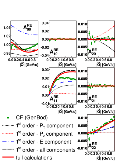
Figures 14 shows the $\pi-p$ correlation function. Since the underlying single-particle proton and pion distributions are isotropic, $A_{1,0}$ (sensitive to shape elongation in $C(\vec{q})$ in $q_{l}$relative to transverse components) is expected to vanish. $A_{1,1}$ is finite, however, due to differences in $p_{T}$ distributions. Since there is no other source of correlation in the simulation, this obviously is an EMCIC.

From Figure 14 it is also clear that neither Equation 24 nor its first-order expansion 25 fully describes the correlation function. This is due to the fact that our formalism is built on the assumption that all particles in the system follow the same parent distribution, as pointed out after Equation V.2.

VIII Summary

To truly claim an understanding of the bulk nature of matter at RHIC and the LHC, a detailed picture of the dynamically-generated geometric substructure of the system created in heavy ion collisions is needed. It is believed that this substructure, and the matter itself, is dominated by strong collective flow. The most direct measure of this flow is a measurement of the space-momentum correlation (e.g. $R\left(m_{T}\right)$) it generates. The physics of this large system, and the signals it generates, should be compared to the physics dominating $p+p$ collisions, as is increasingly important in high-$p_{T}$ studies at RHIC. For small systems, however, non-femtoscopic effects contribute significantly to the correlation function, clouding the extraction and interpretation of femtoscopic ones.

We have discussed a spherical harmonic representation of the correlation function which clearly separates components of the three-dimensional shape measured in modern experiments. This representation is maximally efficient, inasmuch as only a few one-dimensional plots need be examined to extract full 3-D shape information. The relevant number of such plots is further reduced due to symmetry conditions, discussed in detail in Appendix B.

EMCICs, correlations generated by kinematic conservation laws, are surely present and increasingly relevant as the event multiplicity is reduced. Using the code genbod to study correlation functions solely driven by EMCICs, we found highly non-trivial three-dimensional structures strongly influenced by event characteristics (multiplicity and energy) and kinematic particle selection.

We extended the work of Danielewicz, Ollitrault and Borghini to include four-momentum conservation and applied it to correlation functions commonly used in femtoscopy. We found structures associated individually with the conservation of the four-momentum components, which interfere in nontrivial ways. Comparison of the analytic EMCIC calculations with the genbod simulation gave confidence that the approximations (e.g. “large” multiplicity $N$) entering into the calculation were sufficiently valid, at least for multiplicities considered here. We further showed that the full EMCIC calculation can safely be replaced with a first-order expansion in $1/N$.

Based on this first-order expansion, we developed a practical, straight-forward “experimentalist’s formula” to generate histograms from the data which are later used in a generalized fit to the measured correlation function, including EMCICs and femtoscopic correlations. The degree to which this functional form fully describes measured experimental correlation functions has not been discussed and will need exploration on a case-by-case basis.

There is strong interest in correlations between non-identical particles, for two reasons. Firstly, sometimes $\pi^{-}-\pi^{-}$ correlations are divided by $\pi^{+}-\pi^{-}$ correlations in an attempt to “divide out” EMCICs. (In such a procedure, resonance regions are avoided, naturally.) We discussed potential problems with such an approach, related to entrance-channel asymmetries coupled with EMCICs. Secondly, 3-D asymmetries (sometimes quantified as “double ratios”, e.g. Adams:2003qa ) in the correlation function for different-mass particles (e.g. $\pi-K$) are often interpreted in terms of dynamically-generated differences in the average space-time emission point between the two particles. Using a very simple example, we discussed that EMCICs might significantly cloud such an interpretation.

The huge systematics of results and interest in femtoscopy in heavy ion collisions is renewing similar interest in the space-time signals from $p+p$ collisions. Direct comparisons between the two systems are now possible at RHIC and have already produced intriguing preliminary results. Very soon, $p+p$ collisions will be measured in the LHC experiments, and the heavy ion experimentalists will be eager to apply their tools. The femtoscopic tool is one of the best in the box– so long as we keep it sufficiently calibrated with respect to non-femtoscopic effects increasingly relevant in small systems.

Appendix A EMCIC effects on $v_{2}$

Figure 15: (Color online) $v_{2}(p_{T})$ for different event multiplicities. See text for details.

Since EMCICs can produce a structure in the correlation function even in the absence of femtoscopic correlations, it is worthwhile to check analytically and then confirm with simulations whether $v_{2}$– a common measure of collective elliptic flow Ollitrault:1992bk – may be affected by EMCICs.

When calculating flow from two-particle correlations we have the following relations

$$\int\cos\big{(}m\Delta\phi\big{)}\cos\big{(}n\Delta\phi\big{)}d\Delta\phi=\delta_{m,n}\pi,$$ (31)

where for $v_{2}$, $n=2$.

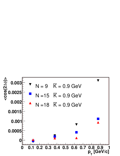
This means that in the absence of flow all EMCIC terms vanish except for the ones that exhibit $\cos\big{(}2\Delta\phi\big{)}$ dependence of $\Delta\phi$. For example in the first order expansion of EMCICs (see Eq. 24) there is a term $\vec{p}_{T,1}\vec{p}_{T,1}\sim\cos\big{(}\Delta\phi\big{)}$. This term gives no contribution to $v_{2}$, nor do any other terms from $1/N$ expansion. The first term that gives a non-zero contribution to $v_{2}$ (means, goes like $\cos\big{(}2\Delta\phi\big{)}$) is the second order expansion term in $\vec{p}_{T}$ that is proportional to $\big{(}\vec{p}_{T,1}\vec{p}_{T,1}\big{)}^{2}\sim\cos^{2}\big{(}\Delta\phi\big{)}\sim\cos\big{(}2\Delta\phi\big{)}$. This term (as well as a few other terms in higher-order $1/N$ expansion) will give a non-zero contribution to $v_{2}$. In our genbod simulations we do not have a flow so we can study the magnitude of the EMCIC effects on $v_{2}$ measurements. Such results are presented on Figure 15 where we plot $v_{2}$ vs $p_{T}$ for three different event multiplicities while the free kinetic energy per particle is fixed ($\bar{K}=0.9~{}GeV$).

As seen, the magnitude of a non-flow contribution to $v_{2}$ from EMCICs is getting smaller with increasing multiplicity and even for low-multiplicity events the magnitude is of order of a few per-mile for large $p_{T}$. From this dependence we can predict that this effect will be so small in heavy ion collisions that it can be simply neglected.

Appendix B Symmetry Considerations

The spherical harmonic decomposition representation, in which three-dimensional correlation functions are represented by several one-dimensional moments, $A_{l,m}$, efficiently condenses the shape information. A much greater increase in efficiency comes, however, with the realization that many $A_{l,m}$’s must vanish by symmetry, depending on the cuts and conditions of the analysis. Besides reducing information by significant factors, this realization also provides diagnostic power– non-physical artifacts often appear in $A_{l,m}$’s which do not vanish when they should. Digging out such effects in the traditional three-dimensional Cartesian representation can be quite difficult.

In the most general case, the 3-D correlation function may have any shape, with no symmetry constraints. In this case, none of the $A_{l,m}$’s need vanish. Usually, however, an analysis is less than fully general, and symmetry consequences then arise.

In particular, we will consider four common conditions used in practice:

1. One measures correlations between identical particles

2. The measurement covers a symmetric rapidity region about y=0 and the collision is between identical ions (e.g. Au+Au rather than Au+Si)

3. The measurement is integrated over reaction-plane angle

4. The measurement might be correlated with the second-order reaction-plane, but the first-order reaction-plane is not known. In other words, the direction of the impact parameter is known at best only modulo $\pi$.

Our strategy begins by identifying transformations in relative momentum $\vec{q}$ under which the measured correlation must be invariant. As an example, since the overall sign of $\vec{q}$ is meaningless when discussing pairs of identical particles (condition [A]), $C\mbox{$\left({}\mbox{$q_{o}$},{}\mbox{$q_{o}$},{}\mbox{$q_{l}$}\right)$}=C\mbox{$\left({-}\mbox{$q_{o}$},{-}\mbox{$q_{o}$},{-}\mbox{$q_{l}$}\right)$}$, or, in spherical coordinates, $C(Q,\cos\theta,\phi)=C(Q,-\cos\theta,\phi-\pi)$.

We then use a symmetry of the spherical harmonics, here $\mbox{$Y_{l,m}\left({}\cos\theta,{}\phi{}\right)$}=(-1)^{l}\mbox{$Y_{l,m}\left({-}\cos\theta,{}\phi{+\pi}\right)$}$ to find

$${\mbox{$A_{l,m}$}}(Q)\equiv\frac{1}{4\pi}\int^{2\pi}_{0}d\phi\int^{1}_{-1}d\cos\theta C(Q,\cos\theta,\phi)\mbox{$Y_{l,m}\left({}\cos\theta,{}\phi{}\right)$}$$

$={\displaystyle \frac{1}{4\pi }}{\displaystyle {\int }_0^{2\pi }}𝑑\varphi {\displaystyle {\int }_{-1}^1}d\cos \theta C(Q,-\cos \theta ,\varphi -\pi )Y_{l,m}(\cos \theta ,\varphi )$

References

- (1) John Adams et al. Nucl. Phys. A757:102–183, 2005
- (2) K. Adcox et al. Nucl. Phys. A757:184–283, 2005
- (3) B. B. Back et al. Nucl. Phys. A757:28–101, 2005
- (4) I. Arsene et al. Nucl. Phys. A757:1–27, 2005
- (5) Jean-Yves Ollitrault. Phys. Rev. D46:229–245, 1992
- (6) M.A. Lisa, S. Pratt, R. Soltz, and U. Wiedemann. Ann. Rev. Nucl. Part. Sci. 55:311, 2005
- (7) S. Pratt. Phys. Rev. Lett. 53:1219–1221, 1984
- (8) F. Retiere and M.A. Lisa. Phys. Rev. C70:044907, 2004
- (9) S. S. Adler et al. Phys. Rev. Lett. 91:072301, 2003
- (10) John Adams et al. Phys. Rev. Lett. 91:172302, 2003
- (11) C. Adler et al. Phys. Rev. Lett. 90:082302, 2003
- (12) C. Derreth, W. Greiner, H. T. Elze, and J. Rafelski. Phys. Rev. C31:1360–1364, 1985
- (13) H. T. Elze and W. Greiner. Phys. Lett. B179:385–392, 1986
- (14) F. Becattini and U. Heinz. Z. Phys. C76:269, 1997
- (15) P. Braun-Munzinger, D. Magestro, K. Redlich, and J. Stachel. Phys. Lett. B518:41–46, 2001
- (16) Ekkard Schnedermann, Josef Sollfrank, and Ulrich W. Heinz. Phys. Rev. C48:2462–2475, 1993
- (17) John Adams et al. Phys. Rev. Lett. 92:112301, 2004
- (18) John Adams et al. Phys. Rev. C72:014904, 2005
- (19) J. D. Bjorken. FERMILAB-PUB-82-059-THY
- (20) Richard M. Weiner. Int. J. Mod. Phys. E15:37–70, 2006
- (21) S. M. Troshin and N. E. Tyurin. hep-ph/0609248
- (22) Gideon Alexander. Rept. Prog. Phys. 66:481–522, 2003
- (23) W. Kittel and E. A. De Wolf. Soft Multihadron Dynamics, Hackensack, USA: World Scientific (2005) 652 p
- (24) Z. Chajecki. AIP Conf. Proc. 828:566–571, 2006
- (25) N. M. Agababyan et al. Z. Phys. C71:405–414, 1996
- (26) M. Gazdzicki and S. Mrowczynski. Z. Phys. C54:127–132, 1992
- (27) Oleg Utyuzh, Grzegorz Wilk, and Zbigniew Wlodarczyk. Phys. Rev. D75:074030, 2007
- (28) G. F. Bertsch, P. Danielewicz, and M. Herrmann. Phys. Rev. C49:442–451, 1994
- (29) F. James. CERN-68-15, http://doc.cern.ch/cernrep/1968/1968-015/1968-015.html
- (30) H. Sorge, Horst Stoecker, and W. Greiner. Nucl. Phys. A498:567c–576c, 1989
- (31) R. Hagedorn. Relativistic Kinematics, N.Y. Benjamin, 1963, 166pp
- (32) Enrico Fermi. Prog. Theor. Phys. 5:570–583, 1950
- (33) S. Pratt. Phys. Rev. D33:1314–1327, 1986
- (34) G. Bertsch, M. Gong, and M. Tohyama. Phys. Rev. C37:1896–1900, 1988
- (35) P. Danielewicz et al. Phys. Rev. C38:120–134, 1988
- (36) Nicolas Borghini, Phuong Mai Dinh, and Jean-Yves Ollitrault. Phys. Rev. C62:034902, 2000
- (37) Nicolas Borghini. Eur. Phys. J. C30:381–385, 2003
- (38) Nicolas Borghini. Phys. Rev. C75:021904, 2007
- (39) Arthur M. Poskanzer and S. A. Voloshin. Phys. Rev. C58:1671–1678, 1998
- (40) D.A. Brown and P. Danielewicz. Phys. Lett. B398:252–258, 1997
- (41) Z. Chajecki. Nucl. Phys. A774:599–602, 2006
- (42) P. Avery et al. Phys. Rev. D32:2294–2302, 1985
- (43) G. Abbiendi et al. Eur. Phys. J. C52:787–803, 2007
- (44) S. Chekanov et al. Phys. Lett. B583:231–246, 2004
- (45) John Adams et al. Phys. Rev. Lett. 91:262302, 2003
- (46) R. Lednicky, V. L. Lyuboshits, B. Erazmus, and D. Nouais. Phys. Lett. B373:30–34, 1996
- (47) Torbjorn Sjostrand et al. Comput. Phys. Commun. 135:238–259, 2001
- (48) M. A. Lisa et al. Phys. Lett. B496:1–8, 2000
- (49) Michael Annan Lisa, Ulrich W. Heinz, and Urs Achim Wiedemann. Phys. Lett. B489:287–292, 2000
- (50) Scott Chapman, Pierre Scotto, and Ulrich W. Heinz. Phys. Rev. Lett. 74:4400–4403, 1995
- (51) Claude Elwood Shannon. Proc. Institute of Radio Engineers. 37:10–21, 1949
- (52) Abdul J. Jerri. Proc. of IEEE. 65:1565–1596, 1977
- (53) David Brown. in preparation. Private comm.
- (54) P. Danielewicz and S. Pratt. Phys. Lett. B618:60–67, 2005
- (55) Pawel Danielewicz and Scott Pratt. Phys. Rev. C75:034907, 2007
- (56) Ulrich W. Heinz, A. Hummel, M. A. Lisa, and U. A. Wiedemann. Phys. Rev. C66:044903, 2002