On composite systems of dilute and dense couplings

Abstract

Composite systems, where couplings are of two types, a combination of strong dilute and weak dense couplings of Ising spins, are examined through the replica method. The dilute and dense parts are considered to have independent canonical disordered or uniform bond distributions; mixing the models by variation of a parameter $\gamma$ alongside inverse temperature $\beta$ we analyse the respective thermodynamic solutions. We describe the variation in high temperature transitions as mixing occurs; in the vicinity of these transitions we exactly analyse the competing effects of the dense and sparse models. By using the replica symmetric ansatz and population dynamics we described the low temperature behaviour of mixed systems.

1 Introduction

Understanding phenomena arising in many body systems through mean field analysis of simple models has provided insight into many problems in physics, theoretical computer science, telecommunication, biology and elsewhere [MPV87, Nis01]. Statistical mechanics describes aspects of macroscopic behaviour in interacting systems of many elements, and methods originating in the study of spin-glasses (SG) have been extended to explore many interesting model disordered systems. These statistical descriptors of behaviour often prove to be a sufficient descriptor of all interesting bulk behaviour; in some applications, such as channel coding and theoretical computer science, they also provide benchmarks even where the large system is relatively small and the randomness assumed does not quite match the true system conditions. Moreover, methods developed within the statistical physics community gave rise to the development of efficient inference algorithms widely used in telecommunication, probabilistic modelling and theoretical computer science.

Many of these models consider range-free interactions of a single topological type, most commonly nearest neighbour interactions in finite dimensional, fully connected, or sparse random graphs. Even in systems not conforming strongly to the particular topology, insight into many phenomena can be obtained and the formulations can allow for exact analysis. We propose that certain systems may be well described by a combination of two canonical topologies – such a property may be phenomenological or could be a deliberately engineered feature of a system.

Amongst the best understood topologies are those amenable to mean field theory models that are infinite dimensional. The canonical mean field model is that of a fully connected graph. This model may be analysed exactly for the cases of uniform interactions and certain random ensembles, most famously the celebrated Sherrington Kirkpatrick (SK) model [SK75]. Simplification of the analysis in the disordered case is often possible through noting the ability to describe many combinations of interactions by a Gaussian due to the central limit theorem. The sparse mean field model has each spin coupled only to a small number of other spins. This creates a topology that is also described as infinite dimensional though the model is perceived as more representative of most complex systems due to some notion of a neighbourhood being maintained. Analysis is simplified by utilising the asymptotic cycle free property (Bethe approximation) of certain random graph ensembles. Models which do not allow use of the Bethe approximation or central limit theorem are in general difficult to analyse.

The motivation for studying this system is that it is amongst the simplest composite models involving a combination of dilute and dense couplings. We anticipate the understanding of these systems to be important in engineering applications. With miniaturisation of technology, for example computer chips, the paradigm by which the interaction amongst components can be strictly controlled may be invalid. Modelling the effect of non-engineered couplings by independent noise may be invalid in some scenarios, as it is possible that these additional interactions form a strongly correlated network allowing for example non-trivial phase transitions or metastable features. There is also the possibility that systems may be engineered deliberately with a combination of dilute strong, and weak dense interactions either to make them more robust or to exploit specific properties of the composite system. In multi-user channel coding, for instance, this may make the communication process more robust against different types of noise, de-synchronisation or malicious attacks. Only recently, a special case of the system studied here was suggested as a model for studying the resilience of networks against attacks [HM].

The paper is organised as follows. In section 2 we introduce the model studied and basic definitions, followed by an analysis section 3 that explains briefly the derivation based on the replica method. In sections 4 and 5 we investigate the high and low temperature solutions, respectively, followed by a discussion of the numerical solutions obtained via population dynamics section 6. Finally, we will present our conclusions in section 7.

2 The model

We present analysis for an ensemble of disordered systems of $N$ Ising spins ${s_{i}=\pm 1}$. The couplings consists of a strong part which is non-zero on only a fraction $\rho N/2$ of the possible links, and a weak part which is present on all links, this defines the Hamiltonian consisting of sparse and dense parts

$${\cal H}({\mbox{\boldmath{$S$}}})={\cal H}_{S}({\mbox{\boldmath{$S$}}})+{\cal H}_{D}({\mbox{\boldmath{$S$}}})+\sum_{i}h_{i}S_{i}$$ (1)

along with an external field. The dense and sparse parts are taken to be

$${\cal H}_{D}({\mbox{\boldmath{$S$}}}) = -\sum_{\langle ij\rangle}b_{i}b_{j}J^{D}_{\langle ij\rangle}\sigma_{i}\sigma_{j},\ ,$$

$${\cal H}_{S}({\mbox{\boldmath{$S$}}}) = -\sum_{\langle ij\rangle}b^{S}_{i}b^{S}_{j}A_{\langle ij\rangle}J^{S}_{\langle ij\rangle}\sigma_{i}\sigma_{j}\;,$$ (2)

where $\left\langle\right\rangle$ indicates the set of ordered (distinct) indices throughout the paper. Components of the sparse connectivity matrix ${\bf A}$ take the value 1 if a link exists between the corresponding sites and zero otherwise; the coupling matrix ${\bf J}$ takes random values from a given distribution and $b$ determines an artificial disorder (alignment) in the coupling strengths, analogous to the Mattis model [Mat]. For our analysis we can take ${\mbox{\boldmath{$b$}}}^{S}=1$ since only the relative alignment is influential in determining system properties.

2.0.1 Mixing of models

In order to investigate the combination of these subsystems we propose the introduction of two parameters, an inverse temperature $\beta$, and a mixing parameter $\gamma\in(0,1)$. The mixing parameter acts so that the couplings in the sparse part increase monotonically from zero with $\gamma$ to their full value, conversely the couplings of the dense part decrease monotonically to zero. There is some flexibility in how this might be applied, for example if the couplings decrease/increase linearly with $\gamma$ one may write the Hamiltonian as

$${\cal H}({\mbox{\boldmath{$S$}}})=\gamma{\cal H}_{S}({\mbox{\boldmath{$S$}}})+(1-\gamma){\cal H}_{D}({\mbox{\boldmath{$S$}}})+\sum_{i}h_{i}S_{i}\;.$$ (3)

This is the simplest composition method we may use but alternative rescalings of the couplings may also be sensible. Unattractive features include that the ratio of variance to mean (${J_{0}}/{\tilde{J}}$) in coupling strengths is not maintained as $\gamma$ varies.

The mixing of models by rescaling of the couplings is not a unique way to consider the composition of two such systems. A sensible alternative valid in some composite systems would be a doping one, keeping the dense part constant and gradually introducing additional sparse bonds (variation of $A$) [HM].

2.0.2 Definition of the ensemble

We consider different ensembles determined by a set of parameters ${\cal I}=\left\{J_{0},{\tilde{J}},\rho,\phi,h^{S},h^{D},\chi,\bar{b}\right\}$ defined as follows. The model consists of independently generated dense and sparse subsystems. Dense Couplings are sampled independently for each link from a distribution of mean $J_{0}b_{i}b_{j}/N$ and variance ${\tilde{J}}/N$ and non-divergent higher moments (the scaling in $N$ is standard [SK75]). The Mattis model-like part $b$ describes some non-trivial orientation of the spins with $b_{i}=\pm 1$ sampled independently at each site according to the mean ${\bar{b}}$. For the sparse part we have that the connectivity matrix, ${\bf A}$, is a sample from an Erdös-Renyi random graph ensemble [ER70] of mean connectivity $\rho$ with couplings sampled independently for each link from a distribution on the real line, $\phi$, with non-divergent moments, and vanishing measure on zero. The external fields are sampled for each site from a distribution of mean $h^{S}+b_{i}h^{D}$, and variance $\chi^{2}$, the parameters $h_{S}$,$h_{D}$ and $\chi^{2}$ are conjugate variables in the free energy to the order parameters for sparse and dense aligned ferromagnetic moments, and the spin glass moment.

The model contains a wide range of parameters which we believe are sufficient to describe the mixing of many canonical Ising spin mean field models. In the case of $\gamma\rightarrow 0$ the model reduces to the SK model [SK75] (up to artificial disorder), whereas at $\gamma\rightarrow 1$ the model is Viana Bray (VB) [VB85]. By tuning parameters one can also find the ferromagnetic, antiferromagnetic and Mattis models [Mat], the relevant orientation in mixing (${\bar{b}}$) proves important in determining system properties. Small perturbations of the SK and VB models by random Hamiltonians is a subject much studied, especially in the context of temperature variation and stochastic stability [BS07, Par, Tal03]. We understand that the set of perturbations represented by variation of an infinitesimal variation of $\gamma$ from $0$ or $1$ probably falls into the classes which are incapable of changing the structure of thermodynamic states - provided we break any interaction symmetries by addition of small external fields, and so we expect no transitions in these limits, which is both an observed and intuitive assumption.

3 Replica method and exact analysis

3.1 Self-averaged free energy calculation

The analysis is rather standard and is carried out by the replica method, we note only important key steps and definitions in this section. Details of the derivation are found in A. Throughout analysis we consider only the leading order contribution, in $N$, to the free energy density, and in all coefficients we assume the asymptotic value in $n$ where possible for brevity. We first write the free energy function making use of the replica trick [MPV87].

$$f = \lim_{N\rightarrow\infty}-\frac{1}{\beta N}\log\sum_{S_{i},\ldots,S_{N}}\exp\left\{-\beta{\cal H}(S_{1},\ldots,S_{N})\right\}\;,$$

$$= \lim_{N\rightarrow\infty}-\frac{1}{\beta N}\lim_{n\rightarrow 0}\frac{\partial}{\partial n}\prod_{\alpha=1}^{n}\left[\sum_{S^{\alpha}_{i},\ldots,S^{\alpha}_{N}}\exp\left\{-\beta{\cal H}(S^{\alpha}_{1},\ldots,S^{\alpha}_{N})\right\}\right]\;.$$

We are interested in the behaviour of a particular sample drawn from the ensemble described by the parameters ${\cal I}$. We anticipate that a sufficient description of any typical instance will be given by the free energy averaged over instances of the disorder (self averaging assumption).

After taking the quenched averages of couplings and some manipulation of the equation form we are able to describe the self averaged free energy density by

$$\left\langle f\right\rangle=\lim_{N\rightarrow\infty}-\frac{1}{\beta N}\lim_{n\rightarrow 0}\frac{\partial}{\partial n}\int d{\Phi}d{\hat{\Phi}}\exp\left\{-N\Lambda(n,{\cal I},\Phi,\hat{\Phi})\right\}\;,$$ (5)

where ${\Phi,\hat{\Phi}}=\left\{\pi({\mbox{{\boldmath{$\sigma$}}}}),{\hat{\pi}}({\mbox{{\boldmath{$\sigma$}}}}),{\bar{q}}_{\alpha},{\hat{\bar{q}}_{\alpha}},{q_{\left\langle\alpha_{1}\alpha_{2}\right\rangle}},{{\hat{q}}_{\left\langle\alpha_{1}\alpha_{2}\right\rangle}}\right\}$ are the set of integration variables introduced to allow exact site factorisation. These may be invoked as order parameters for various phases. Considering only leading order terms in $N$ one can present $\Lambda$ is in the general composite case of two types of disordered couplings

$$\Lambda = -\sum_{\alpha}{\hat{\bar{q}}_{\alpha}}{\bar{q}}_{\alpha}-\sum_{\left\langle\alpha_{1}\alpha_{2}\right\rangle}{q_{\left\langle\alpha_{1}\alpha_{2}\right\rangle}}{{\hat{q}}_{\left\langle\alpha_{1}\alpha_{2}\right\rangle}}-\sum_{{\mbox{{\boldmath{$\sigma$}}}}}\pi({\mbox{{\boldmath{$\sigma$}}}}){\hat{\pi}}({\mbox{{\boldmath{$\sigma$}}}})-\log\left\langle\sum_{\mbox{{\boldmath{$\sigma$}}}}\exp\left\{\mathcal{X}\right\}\right\rangle_{b}$$

$$- \frac{\rho}{2}\sum_{{\mbox{{\boldmath{$\sigma$}}}}_{1},{\mbox{{\boldmath{$\sigma$}}}}_{2}}\pi({\mbox{{\boldmath{$\sigma$}}}}_{1})\pi({\mbox{{\boldmath{$\sigma$}}}}_{2}){\left(\left\langle\exp\left\{\beta x\sum_{\alpha}\sigma_{1}^{\alpha}\sigma_{2}^{\alpha}\right\}\right\rangle_{\phi(x)}-1\right)}-\frac{\beta^{2}{\tilde{J}}}{2}\left[\frac{1}{2}+\sum_{\left\langle\alpha_{1}\alpha_{2}\right\rangle}({q_{\left\langle\alpha_{1}\alpha_{2}\right\rangle}})^{2}\right]$$

$$- \frac{\beta{J_{0}}}{2}\sum_{\alpha}({\bar{q}}_{\alpha})^{2}-\beta\sum_{\alpha}\left(h^{S}\sum_{\mbox{{\boldmath{$\sigma$}}}}\pi({\mbox{{\boldmath{$\sigma$}}}})\sigma^{\alpha}+h^{D}{\bar{q}}_{\alpha}\right)-\beta^{2}\chi^{2}\left(\frac{1}{2}+\sum_{\left\langle\alpha_{1}\alpha_{2}\right\rangle}{q_{\left\langle\alpha_{1}\alpha_{2}\right\rangle}}\right)\;;$$

$$\mathcal{X} = -\sum_{\alpha}{\hat{\bar{q}}_{\alpha}}b\sigma^{\alpha}-\sum_{\left\langle\alpha_{1}\alpha_{2}\right\rangle}{{\hat{q}}_{\left\langle\alpha_{1}\alpha_{2}\right\rangle}}\sigma^{\alpha_{1}}\sigma^{\alpha_{2}}-{\hat{\pi}}({\mbox{{\boldmath{$\sigma$}}}})\;.$$ (6)

The scaling with $\gamma$ is absorbed in the coupling distribution $\phi$,$J_{0}$ and ${\tilde{J}}$.

From here it is possible to evaluate the integral by the saddle point method anticipating the large $N$ limit. The self-consistent equations obtained by the extremisation of the exponent may be evaluated exactly at high temperature and by a qualified approximation at lower temperature. The saddle point equations for the order parameters are

$${\bar{q}}_{\alpha} = {\cal N}\left\langle\sum_{\mbox{{\boldmath{$\sigma$}}}}b\sigma^{\alpha}\exp{\mathcal{X}}\right\rangle_{b}\;;\qquad{\hat{\bar{q}}_{\alpha}}=-\beta{J_{0}}{q_{\alpha}}-\beta h^{D}$$ (7)

$${q_{\left\langle\alpha_{1}\alpha_{2}\right\rangle}} = {\cal N}\left\langle\sum_{\mbox{{\boldmath{$\sigma$}}}}\sigma^{\alpha_{1}}\sigma^{\alpha_{2}}\exp{\mathcal{X}}\right\rangle_{b}\;;\qquad{{\hat{q}}_{\left\langle\alpha_{1}\alpha_{2}\right\rangle}}=-\beta^{2}{\tilde{J}}{q_{\left\langle\alpha_{1}\alpha_{2}\right\rangle}}-\beta^{2}\chi^{2}$$ (8)

$$\pi({\mbox{{\boldmath{$\sigma$}}}}) = {\cal N}\left\langle\exp{\mathcal{X}}\right\rangle_{b}\;;$$

$${\hat{\pi}}({\mbox{{\boldmath{$\sigma$}}}}_{1}) = -\rho\sum_{{\mbox{{\boldmath{$\sigma$}}}}_{2}}\pi({\mbox{{\boldmath{$\sigma$}}}}_{2}){\left(\left\langle\exp\left\{\beta x\sum_{\alpha}\sigma_{1}^{\alpha}\sigma_{2}^{\alpha}\right\}\right\rangle_{\phi(x)}-1\right)}-\beta h^{S}\sum_{\alpha_{1}}\sigma^{\alpha_{1}}$$ (9)

$${\cal N} = \left\langle\sum_{{\mbox{{\boldmath{$\sigma$}}}}}\exp{\mathcal{X}}\right\rangle_{b}^{-1}$$

from which the conjugate order parameters $\hat{\Phi}$ may be eliminated. This representation is convenient for making general ansatze [Mon98] on the order parameters in (39).

3.2 Alternative formulation

It is useful to represent the exponent (LABEL:Lambda1) by choosing a standard parameterisation for $\pi$ allowing components to be associated with different types of order. One can equivalently generate this representation directly by choosing different order parameters and expansions in the replica calculation, the representation remains a standard one [VB85, WS88]. Working at the saddlepoint we are able to substitute saddlepoint definitions for ${\hat{\pi}}$,${\hat{\bar{q}}_{\alpha}}$ and ${{\hat{q}}_{\left\langle\alpha_{1}\alpha_{2}\right\rangle}}$ to obtain an equation in only $\pi({\mbox{{\boldmath{$\sigma$}}}})$,${\bar{q}}_{\alpha}$ and ${q_{\left\langle\alpha_{1}\alpha_{2}\right\rangle}}$. We then reparameterise $\pi$, the generating function of the order parameters, by the complete expansion

$$\pi({\mbox{{\boldmath{$\sigma$}}}})=1+\sum_{\alpha}{q_{\alpha}}\sigma^{\alpha}+\sum_{\left\langle\alpha_{1}\alpha_{2}\right\rangle}{q_{\left\langle\alpha_{1}\alpha_{2}\right\rangle}}\sigma^{\alpha_{1}}\sigma^{\alpha_{2}}+\sum_{l=3}^{n}q_{\left\langle\alpha_{1}\ldots\alpha_{l}\right\rangle}\sigma^{\alpha_{1}}\ldots\sigma^{\alpha_{l}}\;,$$ (10)

The components ${q_{\left\langle\right\rangle}}$ as well as ${\bar{q}}_{\alpha}$ represent spin-spin correlation order parameters between replica [Nis01]. In the case ${\bar{b}}=1$ the distinction between ${q_{\alpha}}$ and ${\bar{q}}_{\alpha}$ is artificial, as emerges from the calculation. We can rewrite the exponent at the saddlepoint as

$$\Lambda = -\log\left\langle\sum_{\mbox{{\boldmath{$\sigma$}}}}\exp\left\{\mathcal{X}\right\}\right\rangle_{b}+\frac{\beta J_{0}}{2}\sum_{\alpha}({\bar{q}}_{\alpha})^{2}+\frac{\beta^{2}{\tilde{J}}+\rho\mathcal{T}_{2}}{2}\sum_{\left\langle\alpha_{1}\alpha_{2}\right\rangle}({q_{\left\langle\alpha_{1}\alpha_{2}\right\rangle}})^{2}$$

$$+ \frac{\rho\mathcal{T}_{1}}{2}\sum_{\alpha}({q_{\alpha}})^{2}+\sum_{l=3}\frac{\rho\mathcal{T}_{l}}{2}\sum_{\left\langle\alpha_{1}\ldots\alpha_{l}\right\rangle}(q_{\alpha_{1}\ldots\alpha_{l}})^{2}\;.$$

$$\mathcal{X} = \sum_{\alpha}\beta(b({J_{0}}{\bar{q}}_{\alpha}+h^{D})+\rho\mathcal{T}_{1}{q_{\alpha}}+h^{S})\sigma^{\alpha}+\beta^{2}\sum_{\left\langle\alpha_{1}\alpha_{2}\right\rangle}(({\tilde{J}}+\rho\mathcal{T}_{2}){q_{\left\langle\alpha_{1}\alpha_{2}\right\rangle}}+\chi^{2})\sigma^{\alpha_{1}}\sigma^{\alpha_{2}}$$ (11)

$$+ \rho\sum_{l=3}\mathcal{T}_{l}\sum_{\left\langle\alpha_{1}\ldots\alpha_{l}\right\rangle}q_{\alpha_{1}\ldots\alpha_{l}}\sigma^{\alpha_{1}}\ldots\sigma^{\alpha_{l}}\;.$$

up to addition of constants. The quantities $\mathcal{T}_{i}$ are to leading order in $n$

$$\mathcal{T}_{i}=\int d\phi(x)\tanh^{i}(\beta x)\,$$ (12)

with $\phi$ being the coupling distribution. The new order parameters must satisfy the set of coupled saddlepoint equations

$$q_{\langle\alpha_{1}\ldots\alpha_{p}\rangle} = \left\langle{\cal N}\sum_{\mbox{{\boldmath{$\sigma$}}}}\left\{\sigma^{\alpha_{1}}\ldots\sigma^{\alpha_{p}}\right\}\exp{\mathcal{X}}\right\rangle_{b}\;,$$ (13)

with (7) still applying. Non-zero order solutions of many types may exist but solutions are non-trivial except at high temperature and zero exteral fields. In the next section we examine solutions for vanishing external fields $h_{S}=h_{D}=\chi=0$ emergent in the high temperature regime.

4 High temperature solutions at zero external field

In the case of zero external fields there exist phases classified by the set of non-zero order parameters. For the low $\beta$ regime the unique stable solution to these equations is the paramagnetic one (P), with all order parameters zero (13). It is possible to determine a hierarchy of critical temperatures [VB85] for the emergence of different types of non-paramagnetic order solution by writing the saddle point equations (13) in cases with all but one type of order parameter types zero. A single spin (ferromagnetic, F) order emerges subject to a non-zero solution of

$$\left(\begin{array}[]{c}{\bar{q}}_{\alpha}\\ {q_{\alpha}}\end{array}\right)=\left(\begin{array}[]{c}\tanh(\beta J_{0}{\bar{q}}_{\alpha})+{\bar{b}}\tanh(\rho\mathcal{T}_{1}{q_{\alpha}})\\ {\bar{b}}\tanh(\beta J_{0}{\bar{q}}_{\alpha})+\tanh(\rho\mathcal{T}_{1}{q_{\alpha}})\end{array}\right)\;.$$ (14)

A Spin-Glass (SG) order requires a non-zero solution to

$${q_{\left\langle\alpha_{1}\alpha_{2}\right\rangle}}=\tanh((\beta^{2}{\tilde{J}}+\rho\mathcal{T}_{2}){q_{\left\langle\alpha_{1}\alpha_{2}\right\rangle}})\;.$$ (15)

Due to the convexity of the tanh function the criteria is described equivalently by a linear expansion

$$\left[\lambda^{S}=\beta^{2}{\tilde{J}}+\rho\mathcal{T}_{2}\right]>1\;.$$ (16)

Higher order solutions, indicated by $q_{\langle\alpha_{1}\ldots\alpha_{p}\rangle}$ emerge subject to the criteria $\rho\mathcal{T}_{p}>1$, by a similar linearisation to (16). However, no solution of this type can emerge at higher temperature than that indicated by equation (16) as the following inequality holds for arbitrary coupling distribution $\phi$ [VB85]

$$(\beta^{2}{\tilde{J}}+\rho\mathcal{T}_{2})\geq\lambda^{(p)}\;,$$ (17)

defining $\lambda^{(p)}=\rho\mathcal{T}_{p}$ for $p>2$, the inequality becomes strict in the case ${\tilde{J}}>0$.

One can apply similar arguments in convexity to aid solution finding in the second case (14), we will restrict attention to the cases ${\bar{b}}=1$ and ${\bar{b}}=0$. In the first case the right-hand-side of (14) is identical in the two components so that the order emerges uniquely along the direction ${t_{\alpha}}\propto{q_{\alpha}}={\bar{q}}_{\alpha}$. The criteria for a non-zero solution is

$$\left[\lambda^{F}_{+}=\beta J_{0}+\rho\mathcal{T}_{1}\right]>1\;.$$ (18)

For the case ${\bar{b}}=0$ the situation is also relatively simple, by the convexity properties of the $\tanh$ it is sufficient to linearise (15) in ${\bar{q}}_{\alpha}$, ${q_{\alpha}}$. The independent processes can then yield solutions depending on one of two eigenvalues meeting the criteria

$$\left[\lambda^{F}_{\pm}=\frac{1}{2}\left(\beta J_{0}+\rho\mathcal{T}_{1}\pm\sqrt{(\beta J_{0}-\rho\mathcal{T}_{1})^{2}+4{\bar{b}}\beta J_{0}\rho\mathcal{T}_{1}}\right)\right]>1\;,$$ (19)

written to be inclusive of both cases ${\bar{b}}=0$ and ${\bar{b}}=1$ (18). Except in the case of a critical temperature with $\rho\mathcal{T}_{1}=\beta J_{0}=1$ the largest eigenvalue $\lambda^{F}=\lambda^{F}_{+}$ will determine the type of the emergent one spin order. We use the generalised order parameter ${t_{\alpha}}\propto v_{1}{\bar{q}}_{\alpha}+v_{2}{q_{\alpha}}$ to correspond to the mode $\lambda^{F}_{+}$, $v$ depending on the type of Ferromagnetic order. We assume throughout the paper that the discrete symmetry in solutions $\pm{t_{\alpha}}$ is broken by a small external field ($h_{S}$ or $h_{D}$) aligned with the positive solution. When $\lambda^{F}_{+}\approx\lambda^{F}_{-}$ one must consider both ${q_{\alpha}}$ and ${\bar{q}}_{\alpha}$ becoming non-zero simultaneously, the consequences of generalising the following sections’ analysis to include this case are considered in  B.1.

Equations (16),(17) and (19) indicate that for any mixed system (${\tilde{J}}$ or ${J_{0}}\neq 0$) there is a transition at some temperature towards a ferromagnetic or SG phase. The effect of $\rho$, which indicates a percolation in the sparse couplings only if $\rho>1$, generates no obvious criticality in the expressions, except in cases where ${J_{0}}\leq 0$ (${\tilde{J}}=0$) then $\rho$ must exceed $1$ for the possibility of a ferromagnetic (SG) high temperature transition, regardless of bond strength or distribution in the sparse part. In this scenario of negative mean coupling in the dense subsystem, $\lambda^{F}_{+}$ (19) is a convex, not monotonically increasing, function of $\beta$. This means for example that by continuous variation of several ensemble parameters one is able to create a first order Paramagnetic-Ferromagnetic (sparsely aligned) transition, with the upper critical temperature changing discontinuously in $\gamma$. Details may depend on the sparse coupling distribution $\phi$.

There exist a number of alternative rigorous methods to attain such a set of paramagnetic high temperature transition points without the use of replicas. In particular we note the results [Ost06], which allow the high temperature transitions to be found by transformation of a disordered Ising spin model to a uniform interaction Ising model for many topologies, thereby allows easy identification of transition points.

4.1 High temperature auxiliary system

We generate a system to describe the non-Paramagnetic phase in the vicinity of the high temperature transition with either or both $\Delta_{1}=\lambda^{F}_{+}-1$ or $\Delta_{2}=\lambda^{SG}-1$ small and positive, and with $\lambda^{(p)}<1$ and $\lambda^{F}_{-}<1$ (there is only one potentially non-zero ferromagnetic alignment). In this scenario we may describe the leading order behaviour to second order in $\Delta$ exactly by an auxiliary saddlepoint equation - which may be subject to exact analysis. This approach is motivated by related methods for sparse SG [VB85, Mot87].

We first introduce some important definitions chosen to be compatible with [VB85]

$$r_{1} =\frac{1}{\lambda^{F}_{+}}-1\;;\qquad r_{2}=\frac{1}{\lambda^{S}}-1\;;\qquad r_{i>2} =\frac{1}{\lambda^{(i)}}-1\;;$$

$${t_{\alpha}} =\lambda^{F}_{+}(v_{1}{q_{\alpha}}+v_{2}{\bar{q}}_{\alpha})+\beta(v_{1}h^{S}+v_{2}h^{D});\qquad\; Q_{(\alpha_{1}\alpha_{2})}=\lambda^{S}{q_{\left\langle\alpha_{1}\alpha_{2}\right\rangle}}+\beta^{2}\chi^{2}\;;$$ (20)

$$Q_{(\alpha_{1}\alpha_{2}\alpha_{3})} =\lambda^{(3)}q_{{\left\langle\alpha_{1}\alpha_{2}\alpha_{3}\right\rangle}}\;;\qquad Q_{(\alpha_{1}\alpha_{2}\alpha_{3}\alpha_{4})}=\lambda^{(4)}q_{{\left\langle\alpha_{1}\alpha_{2}\alpha_{3}\alpha_{4}\right\rangle}}$$

Notation $()$ is to indicate any permutation in the set of indices, the new order parameters are identical for any ordering of indices. The notation $()$ is dropped for abbreviation in the parameters henceforth. The components of ${\mbox{\boldmath{$v$}}}=(v_{1},v_{2})$ describe the different possible alignments of the ferromagnetic order at the high temperature boundary: $(1,1)$ for ${\bar{b}}=1$ and $(1,0)$ $[(0,1)]$ for ${\bar{b}}=0$ with $\rho\mathcal{T}_{1}<[>]\beta J_{0}$, respectively.

At a certain temperature, the minimum $\beta$ which satisfies either (16) or (19), a new phase continuously emerge from the paramagnetic solution which is either ferromagnetic or SG, respectively. A sufficient description of these solutions in the vicinity of this high temperature boundary is given by an expansion in the restricted set of order parameters: ferromagnetic ${t_{\alpha}}$ and SG $Q_{\alpha_{1}\alpha_{2}}$ under some ansatz. The rescaling of order parameters (20) is to abbreviate the expressions, and we consider the case of negligable external fields in examining the transitions. For $\lambda^{X}<1$ the saddle point solution for the $X^{th}$ order parameter is zero unless there is a non-zero component in the higher order parameters, we say the order is induced. For example a non-zero ${t_{\alpha}}$ induces order in $Q_{\alpha_{1}\alpha_{2}},Q_{\alpha_{1}\alpha_{2}\alpha_{3}}$ when $\lambda^{S},\lambda^{(3)}<1$, and $Q_{\alpha_{1}\alpha_{2}}$ induces order in $Q_{\alpha_{1}\alpha_{2}\alpha_{3}\alpha_{4}}$ when $\lambda^{(4)}<1$. We include order parameters upto $4^{th}$ order, this set is sufficient to describe the leading order behaviours of the phases. These inclusions discriminate the approach from a simple mean field (fully connected) approximation to the correlation structure of the sparse subsystem.

Calculations of the significant higher order parameters through the saddle point equations (13) and of $\Tr\left\langle\exp\mathcal{X}\right\rangle$ are undertaken in B. The auxiliary expression for $\Lambda$ (LABEL:Lambda1) can then be found by expansion in ${t_{\alpha}}$,$Q_{\alpha_{1}\alpha_{2}}$,$Q_{\alpha_{1}\alpha_{2}\alpha_{3}}$,$Q_{\alpha_{1}\alpha_{2}\alpha_{3}\alpha_{4}}$ to significant order as

$$\Lambda = \frac{1}{2}\sum_{\alpha}\left((t_{\alpha}-\beta h)^{2}/\lambda^{F}_{+}\!-\!(t_{\alpha})^{2}\right)\!+\!\frac{1}{4}\sum\left((Q_{\alpha_{1}\alpha_{2}}-\beta^{2}\chi^{2})^{2}/\lambda^{S}-(Q_{\alpha_{1}\alpha_{2}})^{2}\right)\!+\!\frac{r_{3}}{12}\sum Q_{\alpha_{1}\alpha_{2}\alpha_{3}}^{2}$$

$$+ \frac{r_{4}}{48}Q_{\alpha_{1}\alpha_{2}\alpha_{3}\alpha_{4}}^{2}+\frac{1}{12}\sum{t_{\alpha}}^{4}+\frac{1}{2!12}\sum Q_{\alpha_{1}\alpha_{2}}^{4}-\frac{1}{45}\sum{t_{\alpha}}^{6}$$

$$- \frac{1}{2!}\sum t_{\alpha_{1}}t_{\alpha_{2}}Q_{\alpha_{1}\alpha_{2}}+\frac{2}{2!3}\sum t_{\alpha_{1}}^{3}t_{\alpha_{2}}Q_{\alpha_{1}\alpha_{2}}+\frac{1}{2!3}\sum t_{\alpha_{1}}t_{\alpha_{2}}Q_{\alpha_{1}\alpha_{2}}^{3}-\frac{3}{3!}\sum t_{\alpha_{1}}t_{\alpha_{2}}Q_{\alpha_{2}\alpha_{3}}Q_{\alpha_{1}\alpha_{3}}$$

$$- \frac{1}{3!}\sum Q_{\alpha_{1}\alpha_{2}}Q_{\alpha_{2}\alpha_{3}}Q_{\alpha_{1}\alpha_{3}}\!-\!\frac{12}{4!}\sum t_{\alpha_{1}}t_{\alpha_{2}}\!Q_{\alpha_{1}\alpha_{3}}\!Q_{\alpha_{2}\alpha_{4}}\!Q_{\alpha_{3}\alpha_{4}}\!-\!\frac{3}{4!}\sum Q_{\alpha_{1}\alpha_{2}}\!Q_{\alpha_{1}\alpha_{3}}\!Q_{\alpha_{2}\alpha_{4}}\!Q_{\alpha_{3}\alpha_{4}}$$

$$- \frac{3v_{2}}{3!}\sum t_{\alpha_{1}}Q_{\alpha_{2}\alpha_{3}}Q_{\alpha_{1}\alpha_{2}\alpha_{3}}-\frac{v_{2}}{3!}\sum t_{\alpha_{1}}t_{\alpha_{2}}t_{\alpha_{3}}Q_{\alpha_{1}\alpha_{2}\alpha_{3}}-\frac{3}{4!}\sum Q_{\alpha_{1}\alpha_{2}\alpha_{3}\alpha_{4}}Q_{\alpha_{1}\alpha_{2}}Q_{\alpha_{3}\alpha_{4}}\;,$$

where summations are over the unordered distinct indices. The difference in this expression from a simple combination of two fully or sparsely connected systems is in the temperature dependence of terms $\Delta_{1}$, $\Delta_{2}$ and in the entropic terms of coefficient $v_{2}$ – the sparsely induced ferromagnetic/mixed solutions differs at second order.

The simplest solution to this equation, consistent with a non-zero solution and the $n\rightarrow 0$ limit, is a replica symmetric one plus fluctuations: taking ${t_{\alpha}}=t+S_{\alpha}$, $Q_{\alpha_{1}\alpha_{2}}=Q+R_{\alpha_{1}\alpha_{2}}$, $Q_{\alpha_{1}\alpha_{2}\alpha_{3}}=Q_{3}+\delta Q_{\alpha_{1}\alpha_{2}\alpha_{3}}$ and $Q_{\alpha_{1}\alpha_{2}\alpha_{3}\alpha_{4}}=Q_{4}+\delta Q_{\alpha_{1}\alpha_{2}\alpha_{3}\alpha_{4}}$. These fluctuations should be considered independent upto permutations on the set of indices. We may now rewrite the auxiliary free energy (4.1) in terms of the RS solution and fluctuations as

$$\Lambda = \Lambda(t,Q,Q_{3},Q_{4})+\mathcal{W}\sum S_{\alpha}+\mathcal{Z}\sum R_{\alpha_{1}\alpha_{2}}+\mathcal{Z}_{3}\sum\delta Q_{\alpha_{1}\alpha_{2}\alpha_{3}}+\mathcal{Z}_{4}\sum\delta Q_{\alpha_{1}\alpha_{2}\alpha_{3}\alpha_{4}}$$

$$+ \mathcal{A}\sum(S_{\alpha})^{2}+\mathcal{B}\sum S_{\alpha}S_{\beta}\!+\!2\mathcal{C}\sum R_{\alpha\beta}S_{\alpha}+\mathcal{D}\sum R_{\alpha\beta}S_{\gamma}\!+\!\frac{\mathcal{P}}{2}\sum R_{\alpha\beta}^{2}\!+\!\mathcal{Q}\sum R_{\alpha\beta}R_{\alpha\gamma}$$

$$+ \frac{\mathcal{R}}{4}\sum R_{\alpha\beta}R_{\gamma\delta}\!+\!\sum\delta Q_{\alpha\beta\gamma}(X\delta Q_{\alpha\beta\gamma}\!+\!YR_{\alpha\beta}\!+\!ZS_{\alpha})\!+\!\sum\delta Q_{\alpha\beta\gamma\delta}(X_{4}\delta Q_{\alpha\beta\gamma\delta}\!+\!Y_{4}R_{\alpha\beta})\;.$$

The prefactors are chosen to make connection with a standard stability analysis result which we use in the following section [dAT78]. For the RS solution to be a saddlepoint solution the terms linear in the fluctuations must vanish so that:

$$\mathcal{W} =0 =\frac{-\beta h}{\lambda^{F}_{+}}+t\left(r_{1}+Q+\frac{1}{3}t^{2}-2Q^{2}-\frac{2}{15}t^{4}-\frac{4}{3}Qt^{2}+\frac{17}{3}Q^{3}-v_{2}\frac{Q_{3}}{t}(t^{2}+Q)\right)\;$$ (23)

$$\mathcal{Z} =0 =\frac{-\beta^{2}\chi^{2}}{2\lambda^{S}}+\frac{1}{2}r_{2}Q+Q^{2}-\frac{1}{2}t^{2}+2Qt^{2}-\frac{17}{6}Q^{3}+\frac{1}{3}t^{4}-\frac{17}{2}Q^{2}t^{2}+v_{2}Q_{3}t-\frac{3}{2}Q_{4}Q,$$ (24)

$$\mathcal{Z}_{3} =0 =\frac{v_{2}}{r_{3}}(v_{2}t^{3}+3Q)\qquad,\qquad\mathcal{Z}_{4}=0=\frac{3Q}{r_{4}}$$ (25)

These allow paramagnetic ($t=Q=0$), ferromagnetic ($t\neq 0$,$Q\neq 0$) and SG ($t=0$,$Q\neq 0$) solutions.

4.2 Stability near the high temperature transition

The RS solution has $t$ and $Q$ such that the exponent is a local extremum. The saddlepoint is a stable local maxima if the quadratic form, which may be described by a real symmetric Hessian, is positive definite. This is difficult to calculate in the general case with non-zero fluctuations in all the order parameters. Instead we wish to consider a restricted set of fluctuations with $\delta Q_{\alpha_{1}\alpha_{2}\alpha_{3}}=\delta Q_{\alpha_{1}\alpha_{2}\alpha_{3}\alpha_{4}}=0$, thus we are testing coupled instabilities with respect to marginal magnetisations and spin-spin correlations only. This restricts somewhat the set of possible perturbations but provides a concise approximation to the stability properties, including the Replica Symmetry Breaking (RSB) ansatz, we expect to generalise very well to inclusion of more complicated multispin instabilities.

We can in the restricted case calculate the eigenvalues of the quadratic form which are degenerate and only of three types in the limit $n\rightarrow 0$ [dAT78]. The stabilities depend on a combination of coefficients given by

$$\mathcal{A}^{\prime} = \mathcal{A}-\mathcal{B}=\frac{r_{1}}{2}+\frac{1}{2}Q+\frac{1}{2}t^{2}-Q^{2}-\frac{1}{3}t^{4}+\frac{17}{6}Q^{3}+\frac{v_{2}}{r_{3}}\left(\frac{3}{2}Qt^{2}+\frac{v_{2}}{2}t^{4}\right)$$ (26)

$$\mathcal{C}^{\prime} = \mathcal{C}-\mathcal{D}=t\left(-\frac{1}{2}-\frac{17}{2}Q^{2}+2Q+\frac{2}{3}Qt^{2}+\frac{v_{2}}{2r_{3}}\left(3Q+v_{2}t^{2}\right)\right)$$ (27)

$$\mathcal{P} = \frac{r_{2}}{2}+t^{2}+\frac{1}{2}Q^{2}$$ (28)

$$\mathcal{Q} = -\frac{Q}{2}-\frac{t^{2}}{2}+\frac{3}{2}Q^{2}+3Qt^{2}$$ (29)

$$\mathcal{R} = -\left(\frac{3}{2r_{4}}+1\right)Q^{2}-2t^{2}Q,$$ (30)

where we have substituted the definitions (25) for the higher order parameters. These combine to give the longitudinal instabilities

$$\lambda_{\pm}=\frac{1}{2}\left(\mathcal{A}^{\prime}+\mathcal{P}-4\mathcal{Q}+3\mathcal{R}\pm\sqrt{(\mathcal{A}^{\prime}-\mathcal{P}+4\mathcal{Q}-3\mathcal{R})^{2}-8(\mathcal{C}^{\prime})^{2}}\right)\;,$$ (31)

and the replicon instability

$$\lambda_{1}=\mathcal{P}-2\mathcal{Q}+\mathcal{R}\;.$$ (32)

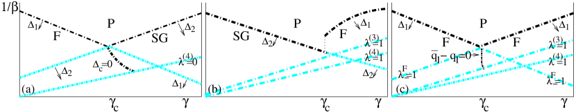
Figure 1: A qualitative description of RS solutions and their instabilities, the auxiliary system results being valid in the vicinity of the high temperature transition line. Dot-dashed lines indicate emergence of high temperature phase transition. The darker (upper) lines indicate the relevant high temperature solution from this set. Left - The high temperature transition can be of ferromagnetic or SG type. If the types of order in the sparse and dense part are not complementary there can exist a triple-point ($\gamma_{C}$). Below the triple-point the type of order will in most cases be that induced by the dense subsystem. The additional dot-dashed line descending from the triple-point corresponds to the RS F-SG transition line (35), the RS ferromagnet being the stable solution between this line and the corresponding Ferromagnetic high temperature transition. The triplepoint analysis is valid where $\lambda^{(p)}<1$. One can reverse the labelling F,SG and corresponding $\Delta$ symbols in the diagram, with the qualitative nature of the diagram being similar. Centre - In cases where the dense distribution has negative mean coupling the ferromagnetic solution to (19) may disappear discontinuously, so that the high temperature transition is a discontinuous one, the triple-point analysis applies to no part of the diagram. Right - In the case of competing alignments of ferromagnetic order then there will exist competition between these alignments; again at a triple-point, the solution below this point can have $({q_{\alpha}},{\bar{q}}_{\alpha})$ non-zero in a combination determined by (14), the free-energy is symmetric about a dotted line $\beta J_{0}=\rho\mathcal{T}_{1}$ at leading order in $\Delta$. This is a vertical line in the $\beta-\gamma$ plane at leading order.

By an expansion of the coefficients, in terms of $\Delta_{2}=\lambda^{S}-1$ near the SG boundary and $\Delta_{1}=\lambda^{F}_{+}-1$ in the vicinity of a ferromagnetic boundary, it is possible to determine leading order RS solutions and their stability properties. We consider the two cases that one component is small and the other large, and the case of a fine balance between the two ($\Delta_{1}=O(\Delta_{2})$). Results should be interpreted with reference to figure 1.

4.3 Solutions below the high temperature transitions

4.3.1 Paramagnetic (P) solution.

The P solution ($t=0,Q=0$) is unstable everywhere below the high temperature transition point and stable everywhere above it; eigenvalues being proportional to $-\Delta_{1}$ and $-\Delta_{2}$.

4.3.2 Ferromagnetic (F) solution.

In the regime where $\Delta_{2}\ll 0$ and $\Delta_{1}>0$, only the F and P solutions exist, one finds the F solution to leading order has $r_{2}Q=t^{2}=3r_{2}\Delta_{1}/(3+r_{2})$. The longitudinal ($\lambda_{+}$), and replicon eigenvalues are proportional to $r_{2}$, which is positive in this regime. The other longitudinal eigenvalue is proportional to $\Delta_{1}$, which is positive and coincident with the high temperature boundary.

4.3.3 Spin Glass (SG) solution.

In the regime where $\Delta_{1}\ll 0$ and $\Delta_{2}>0$ only the SG and P solutions exist. The paramagnetic solution is unstable in a longitudinal mode corresponding to the high temperature boundary. One finds the SG solution gives $Q=\Delta_{2}/2,t=0$ to leading order. The longitudinal eigenvalue $\lambda_{+}$ is coincident with $r_{1}$, which is positive. The other longitudinal eigenvalue is proportional to $\Delta_{2}$, which is positive. The replicon instability is given to leading order as

$$\lambda_{1}=\Delta_{2}^{2}\left(-\frac{3}{8}-\frac{1}{6r_{4}}+\frac{9}{8r_{4}^{2}}\right),$$ (33)

which may be negative or positive depending on the value $r_{4}$. The expected replica symmetry breaking instability is attained when ${\tilde{J}}$ or $\rho$ is large, but where $\rho$ is near the percolation threshold and with ${\tilde{J}}$ small the spin glass can be stable. Since our analysis includes the VB model as a special case, which is prooven to be unstable in the RS spin glass solution  [Mot87], this result must indicate some pathology in the stability analysis – the failure to consider higher order fluctuations. Nevertheless our results may be indicative of a general weakening of instabilities as the sparse coupling limit is approached.

4.3.4 Co-emergence regime $\lambda^{S}\approx\lambda^{F}$.

In this case we make an expansion with both $\Delta_{1}$ and $\Delta_{2}$ small, and consider both the SG and F solution. The SG solution and eigenvalues are unchanged at leading order except in

$$\lambda_{-}=\frac{\Delta_{1}}{8}\left(3\mu-2-\sqrt{4+4\mu+\mu^{2}}\right)+\Delta_{1}^{2}\left(\frac{9}{4r_{4}^{2}}+\frac{5}{12r_{4}}-\frac{1}{2}+O(2-\mu)\right)$$ (34)

where $\Delta_{2}=\mu\Delta_{1}$. This coefficient is negative provided $0<\mu<2$, so a longitudinal instability emerges when

$$\left[\Delta_{c}=\Delta_{1}-\Delta_{2}/2\right]=0\;.$$ (35)

The ferromagnetic solution is changed in both the RS order parameters

$$t^{2}=2\Delta_{1}^{2}-\Delta_{1}\Delta_{2}\qquad;\qquad Q=\Delta_{1}+\Delta_{1}^{2}\left(\frac{1+\mu}{3}+\frac{3v_{2}}{r_{3}}\right)$$ (36)

at leading orders, and in eigenvalues

$$\lambda_{-} = \Delta_{1}\frac{2-\mu}{2}+\Delta_{1}^{2}\left(\frac{3v_{2}}{2r_{3}}\right)+\Delta_{1}^{2}O(2-\mu)$$ (37)

$$\lambda_{1} = \Delta_{1}\frac{2-\mu}{2}+\Delta_{1}^{2}\left(-\frac{1}{2}-\frac{3}{2r_{4}}+\frac{3v_{2}}{r_{3}}+\frac{4(\mu-2)}{3}+\frac{(\mu-2)^{2}}{2}\right)$$ (38)

The other eigenvalue remains coincidence with $\Delta_{1}$ for all $\mu$ (indicating stability). Thus at leading order we have a transition from an $RS$ ferromagnetic system to a longitudinally stable SG when $\mu=2$ (35).

Consider first the situation in which at the triple point $r_{3}$ is not sufficiently small in comparison with $r_{4}$ to make (38) positive, or that the alignment of the ferromagnetic moment is in the dense part $v_{2}=0$. The second order corrections to the eigenvalues for the ferromagnetic regime indicate that in the vicinity of the transition the replicon mode (38) is more negative than the non-negative valued longitudinal mode (37). We have a negative value for the replicon instability, but positive value for the longitudinal stability on the critical line, so that at second order we can predict the existence of a RSB unstable phase of non-zero magnetic moment (a mixed phase, M) between the ferromagnetic and SG solutions in a region about the critical line. This result is qualitatively similar to the Viana Bray (sparse) model stability result for variation of $\rho$ [VB85]. If the replicon eigenvalue is positive on the critical line the mixed phase may be shifted marginally about the critical line. Unfortunately the term $r_{3}$ is sufficiently small to cause positivity in the second order term for many ensembles. A similar complicated dependence of the longitudinal mode exists for the spin glass solution 34 – the results in combination suggest existence of some systems with longitudinally stable F-SG coexistence regimes, rather than a mixed state, near the critical line. However, we suspect these details to be artefacts of the restricted stability analysis.

4.4 Concluding remarks on high temperature solutions

The RS ferromagnetic solution is the unique stable RS solution where it exists, except near the SG transition point (35). The SG RS solution is we suspect an unstable one in the replicon mode, although the stability analysis indicates that at higher temperature there may be a region in which it is an RS stable solution. The paramagnetic solution is unstable everywhere below the high temperature transition lines. The ferromagnetic phase becomes unstable to replica symmetry breaking (in $\left\{{t_{\alpha}},Q_{\alpha_{1}\alpha_{2}}\right\}$) in the vicinity of the transition, generating a mixed phase.

It is of course essential to consider the line (35) represented in terms of some variation of our parameters. This line may be calculated to leading order as a function of $\delta\gamma$ and $\delta\beta$, which is undertaken in C. In so doing we find the line is typically orientated towards $\gamma$ greater than $\gamma_{C}$ as temperature is lowered, indicating a transition from ’dense’ to ’sparse’-type order; a result which is applicable for either type of order (SG or F) in the dense part. This result also implies, interestingly, that ergodicity breaking may disappear as temperature is lowered; a sufficient dense-coupling tendency towards ferromagnetism may allow such a transition in the case of weakly ordered sparse SG. One can consider higher order corrections to the eigenvalues in the vicinity of the triple-point, and in so doing we expect that in most cases a mixed solution will be found, that in some region of parameter space the RS ferromagnetic solution will be unstable when second order corrections are included.

This analysis leaves open the corrections to the stability analysis due to higher order parameters, and results at second order: (34),(38) and (34), motivate such a consideration. A sensible way to probe higher order parameters might be to consider other restricted sets of fluctuations, $\delta Q_{\alpha_{1}\alpha_{2}\alpha_{3}}$ a function of $\delta{t_{\alpha}}$ and $\delta Q_{\alpha_{1}\alpha_{2}}$ for example. We have found that complicated terms in $r_{3},r_{4}$ appear also in these cases, but we anticipate increased instability if fluctuations are allowed in all 4 order parameter types. It is likely such an analytic effort would however be better directed to a more general 1RSB formulation solved by numerical methods. The case of a degenerate transition ($\lambda^{F}_{-}\approx\lambda^{F}_{+}$) by a comparable method is considered in B.1.

5 Low temperature results by RS assumption

5.1 Replica symmetric ansatz

The RS ansatz is here applied to the full free energy expression, the order parameters being invariant with respect to relabelling of spins. Returning to our order parameter description in terms of $\pi({\mbox{{\boldmath{$\sigma$}}}})$ we have the standard definitions

$$\pi({\mbox{{\boldmath{$\sigma$}}}})=\int dW(h)\frac{\exp\left\{\beta h\sum_{\alpha}\sigma_{\alpha}\right\}}{2\cosh(\beta h)}\qquad;\qquad{\bar{q}}_{\alpha}={\bar{q}}_{1}\qquad;\qquad{q_{\left\langle\alpha_{1}\alpha_{2}\right\rangle}}=q_{2}$$ (39)

so that $W(h)$ is now a normalised distribution on the real line describing the moments of $\pi({\mbox{{\boldmath{$\sigma$}}}})$, which must be determined. The self consistent equations may then be reexpressed in terms of the set of parameters $W,{\bar{q}}_{1},q_{2}$ at the saddlepoint

$$W(h) \propto \left\langle\prod_{i=1}^{L}\left[\int dW(h_{i})d\phi(x_{i})\right]\delta(h-H)\right\rangle_{b,L,\lambda_{1},\lambda_{2}}$$ (40)

$${\bar{q}}_{1} \propto \int dh\tanh(\beta h)\left\langle b\prod_{i=1}^{L}\left[\int dW(h_{i})d\phi(x_{i})\right]\delta(h-H)\right\rangle_{b,L,\lambda_{1},\lambda_{2}}$$ (41)

$$q_{2} \propto \int dh\tanh^{2}(\beta h)\left\langle b\prod_{i=1}^{L}\left[\int dW(h_{i})d\phi(x_{i})\right]\delta(h-H)\right\rangle_{b,L,\lambda_{1},\lambda_{2}}$$ (42)

$$H = b{J_{0}}{\bar{q}}_{1}+bh^{D}+h^{S}+\lambda_{1}\sqrt{{\tilde{J}}q_{2}}+\lambda_{2}\chi+\frac{1}{\beta}\sum_{i=1}^{L}{\tt atanh}(\tanh(\beta x_{i})\tanh(\beta h_{i}))$$ (43)

The average in $b$ is with respect to ${\bar{b}}$, $\lambda$ averages are over Gaussian distributions of zero mean and unit variance, and $L$ average is over a Poissonian probability distribution of parameter $\rho$. For ${\bar{b}}=0$ one may reduce the expression (41) to a simple one, as a moment of the distribution $W(h)$.

This equation may be solved by the standard method of population dynamics [GBM01], the distribution $W(h)$ is represented at time $t$ by a histogram of $N$ fields $\left\{h_{i}\right\}$, alongside the scalar order parameters ${\bar{q}}_{1}^{(t)}$ and $q_{2}^{(t)}$. During any update step a single field ($i$) is randomly selected and updated according to a sample from the quenched parameters $\left\{L,b,{\mbox{\boldmath{$x$}}},{\mbox{\boldmath{$h$}}},\lambda_{1},\lambda_{2}\right\}$:

$$h_{i}^{(t+1)} = b^{(t+1)}{J_{0}}{\bar{q}}_{1}+b^{(t+1)}h^{D}+h^{S}+\lambda_{1}^{(t)}\sqrt{{\tilde{J}}q_{2}}+\lambda_{2}^{(t)}\chi$$ (44)

$$+ \frac{1}{\beta}\sum_{j=1}^{L}{\tt atanh}(\tanh(\beta x^{t}_{i_{j}})\tanh(\beta h^{t}_{i_{j}}))$$

$$h_{j\neq i}^{(t+1)} = h_{j\neq i}^{(t)}\qquad\;:\qquad b_{j\neq i}^{(t+1)}=b_{j\neq i}^{(t)}\;,$$ (45)

all other fields being left invariant. Following this we must update the other order parameters, the field $h_{i}^{(t)}$ is removed and the new field $h_{i}^{(t+1)}$ is added to obtain

$${\bar{q}}_{1}^{(t+1)} = {\bar{q}}_{1}^{(t)}+b^{(t+1)}\tanh(\beta h_{i}^{(t+1)})-b^{(t)}\tanh(\beta h_{i}^{(t)})$$

$$q_{2}^{(t+1)} = q_{2}^{(t+1)}+\tanh^{2}(\beta h_{i}^{(t+1)})-\tanh^{2}(\beta h_{i}^{(t)})\ .$$ (46)

Note that in the case that ${\bar{b}}\neq 1$ it is necessary to associate with each field in the histogram the sampled disorder $b^{(t)}$ in the relevant field update step, in order that ${\bar{q}}_{1}^{(t+1)}$ may be incrementally updated.

Convergence through this procedure to the correct solution, to within numerical accuracy dependent on $N$, is fairly robust. In order to avoid systematic errors, and attain convergence in a suitable time scale we must carefully choose initial conditions and population size, decide upon convergence criteria, and a sufficient level of sampling, as discussed in D.

The non-variational free energy $\beta\left\langle f\right\rangle$, coincident with $\Lambda$ after the appropriate limits have been taken, may be written as

$$\frac{\partial}{\partial n}\Lambda \doteq -\frac{\rho}{2}\left\langle\log\cosh\beta x\right\rangle+\frac{\rho}{2}\left\langle\log(1+\tanh\beta x\tanh\beta h_{1}\tanh\beta h_{2})\right\rangle-\left\langle\log 2\cosh(\beta h)\right\rangle$$ (47)

$$+ \rho\left\langle\log\cosh{\tt atanh}(\tanh(\beta h)\tanh(\beta x))\right\rangle+\frac{1}{2}\beta J_{0}{\bar{q}}_{1}^{2}-\frac{1}{4}\beta^{2}{\tilde{J}}(1-q_{2})^{2}-\frac{1}{2}\beta^{2}\chi^{2}\;.$$

With appropriate scaling of the coupling distribution $\phi$ and $\gamma$ with $N$ it is possible to show equivalence of the sparse part with the dense part at large connectivity $\rho$.

Other quantities of interest are

$$\left\langle S^{\alpha_{1}}\ldots S^{\alpha_{k}}\right\rangle=\int dW(h)\tanh(\beta h)\;,$$ (48)

where $W(h)$, the auxiliary field distribution, is identical to the local field distribution. A sufficient statistic to describe the field distribution along the dense alignment is ${\bar{q}}_{1}$ combined with $q_{2}$ in the case ${\bar{b}}=0$. The order parameter ${\bar{q}}_{1}$ is related to the correlation of spins, precisely as the mean spin along the alignment,

$${\bar{q}}_{1}=\left\langle\frac{1}{N}\sum_{i}b_{i}\sigma_{i}\right\rangle\;;$$ (49)

this definition is achieved by the derivative of the variational free energy with respect to $h_{D}$. Similarly, the variance in the external fields, $\chi^{2}$, is conjugate to the parameter $q_{2}$ in the replica formalism, and $h_{S}$ to the mean alignment along sparse ferromagnetic orientation. $q_{2}$ (which may also be determined from the local field distribution (48)) is the SG order parameter, ${\bar{q}}_{1}$ and $q_{1}$ represent ferromagnetic type order parameters. More generally it is possible to show that the local field distribution amongst replica spins (48) is analogous to the field distribution for real spins in a typical sample from the ensemble $\mathcal{I}$.

The entropy is an additional physical quantity of interest – it is known that this can become negative at low temperatures in cases where the RS ansatz is insufficient and provides an indication for an over-simplistic assumption. The energy may be determined simply from the free energy as

$$e = \!-\!\rho/2\int d\phi(x)x\tanh\beta x\!-\!{J_{0}}{\bar{q}}_{1}^{2}/2\!-\!\beta({\tilde{J}}q_{2}^{2}\!-\!1)/2\!-\!h_{D}{\bar{q}}_{1}\!-\!h_{S}\int dW(h)\tanh(\beta h)$$ (50)

$$- \rho/2\int dW(h_{1})dW(h_{2})d\phi(x)x\frac{(1-\tanh^{2}(\beta x))\tanh(\beta h_{1})\tanh(\beta h_{2})}{1+\tanh(\beta x)\tanh(\beta h_{1})\tanh(\beta h_{2})}\!-\!\beta\chi(q_{2}\!-\!1)$$

and the entropy calculated by the Helmholtz relation

$$s=\beta(e-\left\langle f\right\rangle)\;.$$ (51)

It is possible to see that these thermodynamic extensive quantities (51),(50) and (47) differ from the summation of two independent VB and SK subsystems only in the saddlepoint value of $W(h)$.

5.2 Longitudinal stability analysis

Recent work has shown that it is also possible to test the so called longitudinal instabilities within the framework of population dynamics. Consider that a solution to the equations (41),(42) and (40) can be found, one can then examine whether the trajectories of fields in the population $\left\{h_{i}\right\}$ are stable against small perturbations. An unstable trajectory is indicative of ergodicity breaking and may be characterised by divergences in certain properties. It has been shown by Kabashima [Kab03] that the method we shall outline directly tests the longitudinal stability eigenvalue in the AT formalism [dAT78] for the simpler case restricted to dense couplings. In a sparse coupled system Rivoire et al [RBMM04] related the divergence in the mean square fluctuation to the determination of SG susceptibility through the fluctuation dissipation relation.

A more general way to test local instabilities in the sparse case is to consider a less restricted ansatz (1-step of replica symmetry breaking (1-RSB) [MPV87]) on the order parameters, and determine if the state found is identical to the simpler ansatz. To our knowledge there is no formalism sufficient to test all longitudinal stabilities for general topologies. We would expect our system to conform to the hierarchy of replica-symmetry broken ansatze, but possibly not be 1-RSB anywhere. We do not attempt to extend the current analysis to the 1-RSB formalism due to the computational difficulties, especially at low temperatures; moreover, we find the RS-based analysis to provide a good description in much of the phase space, and trust it to be indicative of trends even in the replica-symmetry broken phases for the simple statistics studied.

Instability within the population dynamics solution arises out of the microscopic processes occurring in the update equations. In order to correctly define the consequences of microscopic variation it is necessary to reformulate the dense part of the field update  (44) and represent this by the microscopic processes of iteration of a full set of fields on a tree (Bethe Lattice), alongside the sparse process. This is equivalent to a reformulation of the problem as belief propagation [Kab03], and testing the convergence of the dynamics to a unique solution.

It is necessary to represent the dense interactions in the saddlepoint equation (46) by a similar structure to the sparse interactions, as a summation over many spin-spin interactions rather than their statistical average. Here, the saddle point equations of (46) take a microscopic form

$$b\beta{\bar{q}}_{1}+\lambda^{(t)}_{1}q_{2}\rightarrow\frac{1}{\beta}\sum_{j}b^{(t+1)}_{j}{\tt atanh}\left(\tanh(\beta{\bar{x}}^{(t)}_{j})\tanh h^{(t)}_{j}\right)\;,$$ (52)

where ${\bar{x}}^{(t)}_{j}$ are now random samples from the dense coupling distribution (which may be taken as a Gaussian ${\cal N}(J_{0}/N,{\tilde{J}}/N)$), and $b^{(t+1)}_{i}$ is the orientation of the spin on the target site, $j$ runs over all fields excluding those involved in the sparse subsystem. We will now calculate how a small variation in the incoming fields acts to perturb the outgoing field in a particular update.

$$h_{i}^{(t+1)}+\delta h^{(t+1)} = \sum_{j\setminus\left\{i,i_{1}\ldots i_{L}\right\}}\frac{b^{(t+1)}_{i}}{\beta}{\tt atanh}\left(\tanh(\beta{\bar{x}}^{(t)}_{j})\tanh(h_{j}^{(t)}+\delta h_{j}^{(t)})\right)$$ (53)

$$+ \frac{1}{\beta}\sum_{j=1}^{L}{\tt atanh}\left(\tanh(\beta x^{(t)}_{i_{j}})\tanh(h^{(t)}_{i_{j}}+\delta h^{(t)}_{i_{j}})\right)$$

Where $L$, the set of fields $\left\{i_{j}\right\}$, the sparse and dense couplings and the target disorder are random samples in any update. Assuming the perturbations $\delta h$ to be small and knowing the couplings ${\bar{x}}$ we can make a Taylor expansion to linear order obtaining

$$\delta h^{(t+1)}=b_{i}^{(t+1)}\sum_{j\setminus\left\{i,i_{1}\ldots i_{L}\right\}}(1-\tanh\beta h_{i}){\bar{x}}^{(t)}_{j}\delta h^{(t)}_{j}+\sum_{j=1}^{L}\frac{(1-\tanh^{2}(h^{(t)}_{i_{j}}))\tanh(\beta x^{(t)}_{i_{j}})}{1-\tanh(\beta x^{(t)}_{j})\tanh(h^{(t)}_{i_{j}})}\delta h^{(t)}_{i_{j}}\;,$$ (54)

with the indices again referring to the same quenched samples. Using the fact that the first part is a sum of $N-L^{(t)}\approx N$ random variables we can simplify the description of this term by the central limit theorem, describing the processes by a normal distribution of mean and variance

$$\beta{J_{0}}\left\langle(1-\tanh\beta h_{i})\delta h_{i}\right\rangle/N\;;\qquad\beta^{2}{\tilde{J}}\left\langle(1-\tanh\beta h_{i})^{2}\delta h_{i}\right\rangle/N\;,$$ (55)

respectively.

We are interested in two types of quantities for any solution

$$\chi_{1}=\log\left(\frac{\sum\left(\delta h^{(t+1)}_{i}\right)}{\sum\left(\delta h^{(t)}_{i}\right)}\right)^{2}\qquad;\qquad\chi_{2}=\log\left(\frac{\sum\left(\delta h^{(t+1)}_{i}\right)^{2}}{\sum\left(\delta h^{(t)}_{i}\right)^{2}}\right)\;$$ (56)

which characterise linear and non-linear (SG) susceptibilities by analogy with results for sparse [RBMM04] and dense [Kab03] systems. We expect a negative value in $\chi_{1}$ to indicate local linear stability, while a negative value in $\chi_{2}$ indicates local non-linear stability. We expect the non-linear stability to be sufficient to detect ergodicity breaking trends in solutions.

In the case of a paramagnetic solution results may be determined exactly, the linear instability in $\delta h$ is found to correspond to the ferromagnetic solution criteria (19). The non-linear susceptibility is found to coincide with the SG solution criteria (16). Therefore the paramagnetic solution instabilities determined in section 4.2 are reproduced exactly by this method.

Generally we note that by the nature of the population dynamics algorithm there exist a number of noisy effects: (i) Numerical finite precision errors; (ii) The noise arising from the random order in which fields are updated; (iii) the systematic effect of updating first the field $h^{(t)}_{i}$, then ${\bar{q}}_{1}^{(t)}$ and $q^{(t)}_{2}$; (iv) the finite precision in the histogram; and most importantly (v) the random sampling of quenched parameters in each field update. We can therefore expect convergence of our dynamics to limit not only the final precision achieved, but also the set of solutions, to those stable against such perturbations. We assume this class of perturbations to be sufficient to probe the linear stability even in the low temperature regime. Any linear instability should be observable in some moment of the histogram $\left\{h^{(t)}_{i}\right\}$ so provided we test convergence in $W$ effectively we hope to rule out linear instabilities.

For the other phases the instabilities depend on the details of the field distribution. Consider that we have arrived at some fixed point described by $\left\{h^{(t)}_{i}\right\}$. We can test the stability of this point by adding small perturbations $\left\{(\delta h^{(t)}_{i})^{2}\right\}$ and determining $\chi_{2}$ once the dominate modes emerge. Details of the stability analysis implentation are given in D.

6 Numerical results of population dynamics

We employed population dynamics to investigate a number of systems concentrating on those in which we could examine the effects of competing order as both a weak effect (near the high temperature boundary) and a strong effect at lower temperatures. Many critical quantities could not be sufficiently resolved at high temperature primarily for reasons of finite precision, and near the percolation threshold, in our algorithms we present cases with ($\beta/\beta_{c}<10$) and $\rho=2$, $1/\beta_{c}$ being the largest critical temperature (typically $1$ for examples chosen).

6.1 Data format

All data is based on linear spline interpolation of array data. In the figures over the range $\gamma=(0,1)$ we use a point spacing of $(\delta\beta,\delta\gamma)=(0.025,0.025)$. For these diagrams we present results based on a single run from random initial conditions, and plot the mean and error bars (linear spline interpolation based on values at each sample point) over $20$ samples of data. These $20$ samples are selected in successive time steps (a time step is $N$ single field updates, $1$ for each field), following the convergence of the distribution. Therefore, the error bars are not over independent samples, and as such not necessarily well described by an uncorrelated Gaussian distribution, but this assumption gives a first approximation to single time-step fluctuations in the measured state. Each point that did not converge within $500$ time steps is marked by a cross.

Figures that focus on part of the $\gamma$ range use point spacing of $(0.005,0.005)$. We average quantities in these figures over 10 runs based on different seeds for the random number generator (different initial conditions and updates). The data point is taken to be the mean of $20$ samples from each run. Unlike the sampling within a single run (which may be correlated in successive update steps) we can be confident of the independence of these samples conditional on the parameterisation and convergence criteria, and present the mean and error bars for quantities of interest (again interpolation).

Population dynamics is not required in the paramagnetic region, for which simple boundary conditions based on exact knowledge are imposed, this creates some unevenness in certain quantities very close to the boundary. A second source of unevenness is the array like nature of the data points. Finally our convergence criteria appears not strict enough to prevent some systematic errors (drift) near critical regions, otherwise we expect error bars to be representative.

Cases of incomplete convergence are treated for purposes of data collection and interpolation as converged results. Incomplete convergence occurs:(i) in a small number of cases close to critical transitions, (ii) in the case of competing ferromagnetic alignment. After the maximum number of population iterations is completed ($500$) we select the histogram (amongst 4 differing in initial conditions) of minimum free energy which is good in case (ii), but does not resolve case (i). However, we found experimentally that in cases (i) many quantities did not vary greatly in absolute terms between the histograms of different initial conditions, except for some systematic drift in the stability parameter $\chi_{2}$.

6.2 Figures presented and coupling distributions considered

As there is a large number of composite systems that could be considered and analysed, it would be useful to review the choice of the specific cases presented here.

We present data for the several aligned (${\bar{b}}=1$) combinations of sparse and dense subsystems. A mixture of a dense subsystem of ferromagnetic couplings with a sparse SG (figure 2) or anti-ferromagnetic (figure 4) couplings; and the converse, a subsystem of sparse ferromagnetic couplings mixed with a dense subsystem of SG (figure 3) or anti-ferromagnetic (figures 5 and 6) couplings. We also consider the case of two subsystems both with ferromagnetic couplings but unaligned (${\bar{b}}=0$, figures 7 and  8).

The dense couplings are parameterised by $(J_{0},{\tilde{J}})$, so that for example a dense anti-ferromagnetic system is $(-1,0)$ in this notation. The sparse system we choose is the $\pm J$ model, a canonical case convenient for numerical reasons. In this model $\phi$ is bimodal and described by $p$ the probability of sampling $+J$ as opposed to $-J$ for each bond. Therefore the sparse part is parameterised by $(p,J)$ with $\rho=2$, describing the relevant subsystems we present.

Owing to the large variety of parameterisations we are not able to test sufficient systems to be able to make so general statements as are possible in the exact analysis of the high temperature behaviour. However, we believe these systems to be the most intuitive of combinations. We examined the effect of changing the distribution of sparse couplings $\phi$ from $\pm J$ to Gaussian but found only marginal variations.

6.3 Stability Results

Results are generally characterised by a dominance of the dense system below a critical mixing parameter $\gamma_{c}$ which is replaced by a dominance of the sparse system at larger $\gamma$, although the critical value and the specific properties depend on the system studied and the temperature value.

We find that everywhere close to the boundary the longitudinal stability eigenvalue is positive, thus the RS solutions appear to be locally stable, including in the SG phase. The small gap observed for the SG solution between the numerical results obtained from population dynamics and the high temperature transition line is we suspect due to finite size effects in a combination of population size and number of updates. Otherwise the SG solutions are unstable to ergodicity breaking as expected. The RS ferromagnetic solution may also become unstable at sufficiently low temperatures. Therefore it appears that there is a mixed phase as predicted by the stability analysis in which the magnetic moment is non-zero but ergodicity breaking is present. Dense ferromagnetic phases appear less susceptible to this instability.

6.4 The Co-emergence regime: properties on lowering temperature about a P-F-SG triple-point, $\gamma\approx\gamma_{C}$

We can examine the type of order observed as we decrease the temperature from the triple-point, which provides information as to the relative importance of couplings in weakly ordered systems. It appears that in the vicinity of the triple point one can lower the temperature and finds that the type of order present is closer to that induced by the dense couplings in most cases (inline with the predictions of the high temperature analysis). The sparse type order parameter in some cases completely disappears as temperature is lowered.

If the dense type order is ferromagnetic (figure 2) it appears that by lowering temperature a region of ergodicity breaking may be encountered, but the magnetic moment does not disappear; such a scenario describes a mixed phase. Conversely if one lowers the temperature where the high temperature is a sparsely induced ferromagnetic one (figure 3), it is possible not only for the ferromagnet to become unstable towards a mixed phase, but for the magnetic moment to disappear entirely. This characterises a standard reentrant behaviour, as the magnetic moment re-enters the value it had in the paramagnetic phase. For the anti-ferromagnetic SG state (figure 5) there are some indications of transitions from SG to mixed as well as ferromagnetic to mixed transitions as temperature decreases.

A more exotic possibility observed in the simple combination of a dense ferromagnet and sparse SG subsystems (figures 2 and 4) is that a SG phase may become an RS ferromagnet and then a mixed phase as temperature is lowered. The numerical results are inconclusive on this point, but one can combine this with knowledge of the exact transition line result at the boundary (35), and the intuition that ergodicity breaking is more likely at low temperatures in frustrated systems. It is unusual to our knowledge for ergodicity breaking to disappear as temperature is lowered, only for it then to reappear.

6.5 Discontinuous high temperature transitions

Figures  5 and 6 consider scenarios in which the high temperature transition is potentially discontinuous. Where the boundary is discontinuous, the sparse coupling order is ferromagnetic; it appears that the sparse-induced ferromagnetic order overwhelms any emergence of SG order in the vicinity of the discontinuity ($\gamma\approx\gamma_{C}$), so that the SG phase must occupy only some very narrow region about the high temperature transition. We can anticipate for both the SG and paramagnetic phases, that convergence of population dynamics might be subject to especially strong finite size effects in the vicinity of this transition. We vary the sparse ensemble through $J$ to generate the different scenarios, $\rho$ may also be varied to create this effect.

With the transition nearly discontinuous (as is the case for $J=1/2$ figure 5 in which the discontinuity is visually imperceptable) one observes a similar behaviour to the case of a SG-F combination (figure 2) except in the weaker suppression of the ferromagnetic order at low temperatures. Clearly, in this case the antiferromagnetic dense component cannot induce any order except for a paramagnetic one and the emergence of a SG is a property of the sparse distribution.

In figure 6a where a discontinuity is clearly visible we find ergodicity breaking is surpressed in the vicinity of the discontinuity. The ferromagnetic phase dominates near $\gamma_{c}$ at high temperature but gives way to a mixed phase at lower temperature. Figure  6b shows that in the continuous case the high temperature prediction is qualitatively accurate. The SG state appears to dominate near $\gamma_{c}$, with mixed phases appearing at lower temperature.

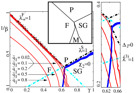
Figure 2: A dense subsystem $(J_{0}=1,{\tilde{J}}=0)$ with a sparse subsystem $(p=0.5,J=1)$ – dense ferromagnetic and sparse SG couplings. A schematic denotes our qualitative understanding of the solutions. Main figure: The exact critical lines ((16),(17),(19)) are indicated by dot dashed lines with the darker (upper) line being the exact high temperature transition. The thick line $\chi_{2}=0$, and the line of zero magnetisation $q_{1}=0$, indicate transition points as determined by the population dynamics algorithm. The continuation of $q_{1}=0$ must be inferred by the contours in $q_{1}$ (thin lines). Error bars in all contour lines are plotted and indicate time-step fluctuations within a single run. Transitions are between unstable-stable and SG-F solutions, the unstable ferromagnetic solution is classified a mixed state. It appears the effect of sparse frustrating bonds is to make the RS dense ferromagnet unstable as $\beta$ increases. Similarly the sparsely induced SG may be susceptible to a transition towards a mixed state with increasing $\beta$. The mixed phase remains close to $\gamma=\gamma_{c}$, thus the competition of interaction types remains in some sense balanced as temperature decreases. Inset figure: The right figure shows the same contours as the main figure in magnification with corresponding error bars (variation between different independent minimisations). We also plot the high temperature critical line (35), which indicates the exact gradient for the curves $\chi_{2}=0$ and $q_{1}^{2}=0$, this appears not to be closely followed by the line $\chi_{2}$ which is due to finite size numerical errors and coarseness of point sampling.

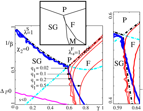
Figure 3: A dense subsystem $(J_{0}=0,{\tilde{J}}=1)$ with a sparse subsystem $(p=1,J=\frac{1}{2})$, i.e., dense SG and sparse uniform ferromagnetic couplings. A schematic denotes our qualitative understanding of the solutions. Main figure: Lines and symbols are the same as for figure 2, in addition the thick dotted line represents a lower temperature bound to positive entropy (include the negligible time-step errors), below this line the method is inconsistent as would be suggested by our results on instability of the SG phase (to which this curve belongs). Inset: The low magnetisation contours, and stability parameter follow quite closely the triple-point analysis prediction (35) in the vicinity of the boundary (inset). These lines break indicating a mixed phase. It appears there may be no transitions in the SG state towards, a mixed phase. The mixed phase is shifted to higher $\gamma$ with increasing $\beta$ indicating the greater relative importance of the dense disordered couplings in determining phase behaviour as temperature is lowered. The ferromagnetic state is first unstable to a mixed state, which may in turn be unstable towards a SG state.

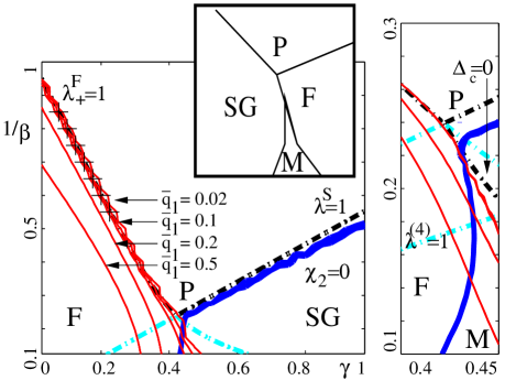
Figure 4: The combination of dense subsystem $(J_{0}=1,{\tilde{J}}=0)$ and sparse subsystem $(p=0,J=\frac{1}{2})$ is a combination of ferromagnetic and antiferromagnetic (SG) effects; lines and symbols are as in the previous figures. Not surprisingly this case is almost identical to the case of figure 2. There is excellent agreement between the thin data lines (ferromagnetic moments) and the high temperature prediction for their disappearance (inset). A clear cusp exists in the stability, indicating that an ergodic ferromagnetic behaviour may emerge in some systems as temperature is lowered, this indicates increasing importance of the dense couplings as temperature is lowered. However, instabilities do reemerge at lower temperature. The SG is susceptible to a mixed state as temperature is lowered.

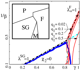
Figure 5: The combination of dense subsystem $(J_{0}=-1,{\tilde{J}}=0)$ and sparse subsystem $(p=1,J=\frac{1}{2})$ is a combination of antiferromagnetic and ferromagnetic effects; lines and symbols as in the previous figures. The dense couplings cannot independently induce SG or ferromagnetic order, but do suppress ferromagnetic order. The resulting behaviour is comparable to a SG ferromagnet combination– figure 3. By contrast to the dense SG coupling there is weaker suppression of the magnetic moment at low temperature, and ergodicity breaking is a weaker effect at low temperature in the ferromagnetic phase. In this diagram the high temperature transition line are marginally discontinuous as discussed (section 6.5). Therefore we do not provide a detailed inset for the triple point analysis region.

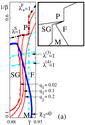
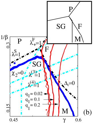
Figure 6: Anti-ferromagnetic couplings in the dense part aligned with ferromagnetic order in sparse couplings can cause the high temperature ferromagnetic solution criteria (18) to be unmet for any $\beta$ in some range of $\gamma$. If 19 describes the high temperature transition as $\gamma$ decreases towards this range then there is a discontinuity (a) and the stability analysis for the region $\Delta_{2}=0(\Delta_{1})$ does not apply, otherwise the transition is a continuous one (b) with the stability analysis applicable. (a) With antiferromagnetic dense couplings $({J_{0}}=-2,{\tilde{J}}=0)$ and ferromagnetic sparse couplings $(p=1,J=1)$, the transition is discontinuous. The sparse order dominates the dense order near $\gamma\approx\gamma_{C}$, the relative importance of the dense couplings increases as temperature is lowered. The closeness of the magnetisation contours to the line $\lambda^{S}=1$ may be a significant finite size effect, these lines do not coincide in the thermodynamic limit. (b) With antiferromagnetic dense couplings $({J_{0}}=-\frac{1}{4},{\tilde{J}}=0)$ and ferromagnetic sparse couplings $(p=1,J=1)$, the transition is continuous. Results appear to follow closely the high temperature prediction. At lower temperature $\gamma\approx\gamma_{C}$ appears to remain approximately coincident with a SG-M transition, the ferromagnet is again unstable to a mixed phase in many systems.

6.6 Unaligned ferromagnetic couplings ${\bar{b}}=0$

This is an interesting case of competing ferromagnetic alignments; as one decreases the temperature in the vicinity of $\gamma_{C}$ it appears that, as a thermodynamic solution, the sparse alignment is marginally dominated in the thermodynamic state by the dense alignment (figure 7). However, the sparse aligned solution persists at lower temperature as a metastable state, responsible for the non-convergence, which is locally stable against ergodicity breaking ($\chi_{2}<0$).

In fact, metastable states of both dense and sparse alignment exist across a wide range of parameters $\gamma$ for any $\beta$ below the triple point (figure 8), indicated by populations converging to different numerically stable solutions. These metastable states are characterised numerically by ${\bar{q}}_{1}>0,q_{1}\approx 0$ and $q_{1}>0,{\bar{q}}_{1}\approx 0$ and we speculate the thermodynamic state involves a first order transition between the two solutions. A necessary condition for the existence of a metastable state is the non-negativity of both $\lambda^{F}_{\pm}-1$, but this is not necessarily sufficient.

Histograms with a well defined alignment tend to converge to the locally stable state with the same corresponding alignment, whether or not this is the thermodynamic solution. Random initial conditions appear to converge towards the thermodynamic solution at high temperature, but have a slight bias towards the dense alignmnent at lower temperatures (atleast over a small number of updates). It is difficult to determine if the solution space generate a larger basin of attraction for the dense metastable state, or one, in some sense, proportional to the free energy. This may be important given that we envisage composite systems as components in optimisation problems were dynamical minimisation by local search, similar to population dynamics, is a critical feature, possibly more so than any static properties of the ensemble.

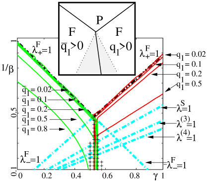
Figure 7: A system with ${\bar{b}}=1$, and uniform couplings of $(J_{0}=1,{\tilde{J}}=0)$ and $(p=\frac{1}{2},J=1)$, models the competition between two unaligned ferromagnetic orderings; lines and symbols as in the previous figures. The converged solutions were found to be ergodic everywhere ($\chi_{2}<0$) and were of positive entropy. In a part of the space below the cusp in the high temperature transition ($\gamma_{c}$) population dynamics converge to one of two differently aligned locally stable states as can be seen by the crosses. Varying $\gamma$ through the centre of this region there is a rapid decline in ${\bar{q}}_{1}$ with the magnetic moment growing instead in $q_{1}$. We speculate that this is a first order transition between two locally stable states.

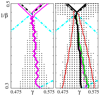
Figure 8: A system with ${\bar{b}}=1$, and uniform couplings of $(J_{0}=1,{\tilde{J}}=0)$ and $(p=\frac{1}{2},J=1)$, models the competition between two unaligned ferromagnetic orderings. These figures show magnifications of figure 7 near $\gamma_{c}$. Left figure: In the vicinity of $\gamma_{c}$ a large number of states fail to converge after maximum algorithm time of $500$ steps (dots). We then have to chose which of the 4 replica histograms evolved in the dynamics produces a result of smallest free energy. If we evaluate the magnetisation in this state we find a transition indicated by change of sign in ${\bar{q}}_{1}-q_{1}$, this is plotted with error bars (time step fluctuations) for a single run. Left figure: Sampling 20 systems with a maximum time of $100$ time steps in each iteration we show the contour ${\bar{q}}_{1}-q_{1}=0$ with sampling errors for several different histograms evolved in parallel: a sparsely aligned ferromagnetic (left most line), random SG or nearly paramagnetic (central thin lines) or densely aligned ferromagnetic initial histogram. The central thicker black line is the equilibrium result as determined by from the histogram of minimum free energy. With only $100$ iterations there is a slightly broader set of unconverged states (dots), but we already see the emergence of two well defined dynamical transitions - left and right lines, matching approximately the result in the left figure. The alignments of the random histograms appear to approximately match the thermodynamical transition at high temperature but are noisy and slightly biased towards a dense alignment at lower temperature.

7 Conclusion

This paper considers the question of systems consisting of a combination of sparse and dense random couplings. Given the complementary properties of these types of structures, combined with the possibility of a robust statistical description, many engineered systems may benefit by a decomposition as laid out here. Such an example we are currently pursuing involves the combination of sparse and dense spreading codes for multiuser access [RS07]. An alternative application of this analysis might be in modelling random attacks on network structures, where correlations between attacked elements are induced [HM].

This paper has considered a simple model in which canonical sparse and dense disordered models have been mixed. In so doing we have observed some clear trends which may generalise. These include the tendency for dense induced order to dominate sparse induced order when in competition. In a system with a dense ferromagnetic tendency, it is possible for this order to emerge from a sparse induced SG as a replica-symmetric stable system by lowering the temperature, provided the order is sufficiently weak (high temperature). In the vicinity of a high temperature transition the effect of suppressing ferromagnetic order by an increasing antiferromagnetic tendency in the bonds may have a very similar effect to the introduction of frustrating effects in the interaction structure. Finally, the case of the unaligned system indicates that the dominance of dense ferromagnetic over sparse ferromagnetic couplings is marginal in equilibrium properties, however it appears a metastable behaviours may have non-trivial consequences for dynamics.

Several questions remain open - importantly, the question of the low temperature limit is not resolved in this paper nor is the behaviour in the vicinity of the percolation threshold. These may be analysed by related statistical physics methods. There are a number of other variations which would allow the insight gained from the current study to be strengthened, including reformulations of the basic model so that the arbitrary parameter $\gamma$ may be shown to be only a technicality; so that related models, for example, in which a dense system is fixed and one gradually adds more bonds (a variation of $\rho$), may be surmised. One can consider a number of ways of scaling $\phi$,$J_{0}$ and ${\tilde{J}}$ with $\gamma$ but we hope the properties we have reported here are robust against the most sensible alternatives such as scaling all coupling moments of each subsystem uniformly with $\gamma$.

Finally, with the increasing interest in complex systems of varying connectivities and interaction strengths, we believe the current study of a simple composite system comprising elements which have both sparse (and strong) and dense (weak) interactions, represents a first step in the principled analysis of their equilibrium behaviour.

Acknowledgments

DS would like to thank Ido Kanter for useful comments. This work is partially supported by EVERGROW, IP No. 1935 in the complex systems initiative of the FET directorate of the IST Priority, EU FP6 and EPSRC grant EP/E049516/1.

Appendix A Replica calculation

A particular ensemble $\mathcal{I}$ is described by a set of order one scalars $\left\{J_{0},{\tilde{J}},\rho,h_{S},h_{D},\chi^{2}\right\}$ and a sparse coupling distribution $\phi$ of finite moments on the real line, without finite measure at zero. These parameters contain an unstated dependence on the mixing parameter, we choose this to be in the couplings $\phi$,$J_{0}$ and ${\tilde{J}}$ but leave this unstated for brevity. An instance of the ensemble is constructed according to the following probability distributions, subscripts being the relevant random variables

$$P_{\mbox{\boldmath{$b$}}}({\mbox{\boldmath{$x$}}}) \propto \prod_{i=1}^{N}\left[\delta_{x_{i},1}(1+{\bar{b}})+\delta_{x_{i},-1}(1-{\bar{b}})\right]\;;$$

$$P_{{\mbox{\boldmath{$J$}}}^{D}}({\mbox{\boldmath{$x$}}}) = \prod_{{\left\langle ij\right\rangle}}\phi^{D}(x_{\left\langle ij\right\rangle})\;;$$

$$P_{{\mbox{\boldmath{$J$}}}^{S}}({\mbox{\boldmath{$x$}}}) = \prod_{{\left\langle ij\right\rangle}}\phi(x_{\left\langle ij\right\rangle})\;;$$

$$P_{{\mbox{\boldmath{$A$}}}}({\mbox{\boldmath{$x$}}}) = \prod_{{\left\langle ij\right\rangle}}\left[\left(1+\frac{\rho}{N}\right)\delta_{x_{\left\langle ij\right\rangle}}+\frac{\rho}{N}\delta_{x_{\left\langle ij\right\rangle},1}\right]\;;$$

$$P_{{\mbox{\boldmath{$h$}}}}({\mbox{\boldmath{$x$}}}) = \prod_{i}\phi^{F}(x_{i})\;.$$

The dense coupling distribution $\phi^{D}$ may be taken as a Gaussian of mean $J_{0}/N$ and variance ${\tilde{J}}/N$. The field distribution for each site is a Gaussian of mean $h_{D}b_{i}+h_{S}$ and variance $\chi^{2}$.

We describe the properties of a particular ensemble through self averaged quantities calculated from the mean free energy density (self averaging assumption) which with the replica identity [MPV87] may be written

$$\left\langle f\right\rangle=\lim_{N\rightarrow\infty}-\frac{1}{\beta N}\lim_{n\rightarrow 0}\frac{\partial}{\partial n}\left\langle Z^{n}\right\rangle\;,$$

with $\beta$ the inverse temperature. The replicated partition function, averaged over samples is given by

$$\left\langle Z\right\rangle = \sum_{{\mbox{\boldmath{$S$}}}_{1}\ldots{\mbox{\boldmath{$S$}}}_{n}}\left\langle\left\langle\exp\left\{\sum_{\alpha}\sum_{\left\langle ij\right\rangle}b_{i}b_{j}J^{D}_{\left\langle ij\right\rangle}\sigma^{\alpha}_{i}\sigma^{\alpha}_{j}\right\}\right\rangle_{{\mbox{\boldmath{$J$}}}^{D}}\left\langle\exp\left\{\sum_{\alpha}\sum_{\left\langle ij\right\rangle}A_{\left\langle ij\right\rangle}J^{S}_{\left\langle ij\right\rangle}\sigma^{\alpha}_{i}\sigma^{\alpha}_{j}\right\}\right\rangle_{{\mbox{\boldmath{$A$}}},{\mbox{\boldmath{$J$}}}^{S}}\right.$$

$$\times \left.\left\langle\exp\left\{\sum_{\alpha}\sum_{i}h_{i}\sigma^{\alpha}_{i}\right\}\right\rangle_{{\mbox{\boldmath{$h$}}}}\right\rangle_{{\mbox{\boldmath{$b$}}}}\;.$$

As is standard in such calculations [MPV87] we maintain only those terms in the exponent which are order $N$, taking asymptotic values in $n\rightarrow 0$ for brevity in all prefactors. The quenched average on dense couplings may be factorised and taken by linearising the exponent, resulting in

$$\left\langle\cdots\right\rangle_{{\mbox{\boldmath{$J$}}}^{D}}=\prod_{\left\langle ij\right\rangle}\exp\left\{\frac{\beta{J_{0}}}{N}b^{\prime}_{i}b^{\prime}_{j}\sum_{\alpha}\sigma^{\alpha}_{i}\sigma^{\alpha}_{j}+\frac{\beta^{2}{\tilde{J}}}{2N}\left(\sum_{\alpha}\sigma^{\alpha}_{i}\sigma^{\alpha}_{j}\right)^{2}\right\}\;.$$

The sparse coupling average may also be taken by standard sparse methods [Mon98]

$$\left\langle\cdots\right\rangle_{{\mbox{\boldmath{$J$}}}^{S},{\mbox{\boldmath{$A$}}}}=\prod_{\left\langle ij\right\rangle}\left[\exp\left\{-\frac{\rho}{N}\right\}\exp\left\{\frac{\rho}{N}\left(\left\langle\exp\left\{\beta x\sum_{\alpha}\sigma^{\alpha}_{i}\sigma^{\alpha}_{j}\right\}\right\rangle_{\phi(x)}\right\}-1\right)\right]\;,$$

and the field average

$$\left\langle\ldots\right\rangle_{{\mbox{\boldmath{$h$}}}}=\prod_{i}\exp\left\{\beta(h^{D}b_{i}+h^{S})\sum_{\alpha}\sigma^{\alpha}_{i}+\beta^{2}\chi^{2}/2(\sum_{\alpha}\sigma^{\alpha}_{i})^{2}\right\}\;.$$

Introducing the following order parameters, $\Phi$:

$$\pi({\mbox{{\boldmath{$\sigma$}}}})=\frac{1}{N}\sum_{i}\delta_{{\mbox{{\boldmath{$\sigma$}}}}_{i},{\mbox{{\boldmath{$\sigma$}}}}}\;;\qquad{\bar{q}}_{\alpha}=\frac{1}{N}\sum_{i}b_{i}\sigma^{\alpha}_{i}\;;\qquad{q_{\left\langle\alpha_{1}\alpha_{2}\right\rangle}}=\frac{1}{N}\sum_{i}\sigma^{\alpha_{1}}_{i}\sigma^{\alpha_{2}}_{i}\;;$$

we are able to write the replicated partition function as an integral in the set of order parameters

$$\left\langle Z^{n}\right\rangle \propto \int d\Phi\sum_{{\mbox{{\boldmath{$\sigma$}}}}_{1}\ldots{\mbox{{\boldmath{$\sigma$}}}}_{N}}\mathbf{I}(\Phi)\exp\left\{-NG_{1}\right\}\;;$$

$$\phantom{G}G_{1} = -\frac{\beta J_{0}}{2}\sum_{\alpha}{\bar{q}}_{\alpha}^{2}-\frac{\beta^{2}{\tilde{J}}}{2}\sum_{\alpha}{q_{\left\langle\alpha_{1}\alpha_{2}\right\rangle}}^{2}-\frac{\rho}{2}\sum_{{\mbox{{\boldmath{$\sigma$}}}}_{1},{\mbox{{\boldmath{$\sigma$}}}}_{2}}\pi({\mbox{{\boldmath{$\sigma$}}}})\pi({\mbox{{\boldmath{$\sigma$}}}})\left\langle\exp\left\{\beta x\sigma^{\alpha_{1}}\sigma^{\alpha_{2}}\right\}-1\right\rangle_{\phi}$$

$$- \beta h_{S}\sum_{\mbox{{\boldmath{$\sigma$}}}}\pi({\mbox{{\boldmath{$\sigma$}}}})\sigma_{\alpha}-\beta h_{D}\sum_{\alpha}q_{\alpha}-\beta^{2}\chi^{2}\sum_{\left\langle\alpha_{1}\alpha_{2}\right\rangle}{q_{\left\langle\alpha_{1}\alpha_{2}\right\rangle}}\;;$$

where the function $\mathbf{I}$ is an indicator function for the order parameter definitions  A. We note here that there is potentially some redundancy in the definition of order parameters, this is allowed for a concise and general expression.

Representing each definition in the indicator function by a Fourier transform, introducing conjugate integration variables denoted with a hat,

$$\sum_{{\mbox{{\boldmath{$\sigma$}}}}_{1}\ldots{\mbox{{\boldmath{$\sigma$}}}}_{N}}\mathbf{I}(\Phi) = \int d\Phi\exp\left\{-N(G_{2}+G_{3})\right\}\;;$$

$$G_{2} = -\sum_{\alpha}{\bar{q}}_{\alpha}{\hat{\bar{q}}_{\alpha}}-\sum_{\left\langle\alpha_{1}\alpha_{2}\right\rangle}{{\hat{q}}_{\left\langle\alpha_{1}\alpha_{2}\right\rangle}}{q_{\left\langle\alpha_{1}\alpha_{2}\right\rangle}}-\sum_{\mbox{{\boldmath{$\sigma$}}}}\pi({\mbox{{\boldmath{$\sigma$}}}}){\hat{\pi}}({\mbox{{\boldmath{$\sigma$}}}})\;;$$

$$G_{3}~{} = -\log\sum_{\mbox{{\boldmath{$\sigma$}}}}\left\langle\exp\left\{-b\sum_{\alpha}{\hat{\bar{q}}_{\alpha}}\sigma^{\alpha}-\sum_{{\left\langle\alpha_{1}\alpha_{2}\right\rangle}}{{\hat{q}}_{\left\langle\alpha_{1}\alpha_{2}\right\rangle}}\sigma^{\alpha_{1}}\sigma^{\alpha_{2}}-{\hat{\pi}}({\mbox{{\boldmath{$\sigma$}}}})\right\}\right\rangle_{b}\;;$$

assuming $N$ is the suitable scaling for the conjugate variables. We have finally a site factorised saddlepoint form (5).

Appendix B Calculation details for auxiliary system

In order to construct the auxiliary system we must determine the significance of terms. We keep terms sufficient to allow a second order description in $\Delta$, which is the perturbation away from $\lambda_{S}=1$ and/or $\lambda^{F}_{+}=1$, and to allow a second order stability analysis, restricted to the region where $\lambda^{(p)}<1$ and $\lambda^{F}_{-}<1$. We calculate the expansion of the complicated entropic term $\log\Tr\exp\left\{\mathcal{X}\right\}$ in equation (11) in the reduced set of order parameters $\left\{{t_{\alpha}},Q_{\alpha_{1}\alpha_{2}},Q_{\alpha_{1}\alpha_{2}\alpha_{3}},Q_{\alpha_{1}\alpha_{2}\alpha_{3}\alpha_{4}}\right\}$ and to an order fit for purpose. This becomes for ${\bar{b}}=1$ ($v_{2}=1$) or ${\bar{b}}=0$ ($v_{2}=1$ or $0$)

$$-\log\Tr\exp\mathcal{X} = \!-\sum\log\cosh{t_{\alpha}}\!-\!\sum\log\cosh{\bar{Q}}_{\left\langle\alpha_{1}\alpha_{2}\right\rangle}$$

$$- \sum\log\cosh Q_{\left\langle\alpha_{1}\alpha_{2}\alpha_{3}\right\rangle}^{2}-\sum\log\cosh Q_{\left\langle\alpha_{1}\alpha_{2}\alpha_{3}\alpha_{4}\right\rangle}^{2}$$

$$- \log\Tr\left\langle\prod\left[1+v_{2}\tanh({t_{\alpha}})\sigma_{\alpha}\right]\right\rangle\prod\left[1+\tanh({\bar{Q}}_{\left\langle\alpha_{1}\alpha_{2}\right\rangle})\prod_{i=1}^{2}\sigma_{\alpha_{i}}\right]$$

$$\times \prod\left[1+\tanh(Q_{\left\langle\alpha_{1}\alpha_{2}\alpha_{3}\right\rangle})\prod_{i=1}^{3}\sigma_{\alpha_{i}}\right]\prod\left[1+\tanh(Q_{\left\langle\alpha_{1}\alpha_{2}\alpha_{3}\alpha_{4}\right\rangle})\prod_{i=1}^{4}\sigma_{\alpha_{i}}\right]\ ;$$

the sums and products are ordered in the various terms and are over the corresponding replica indices. The case of an aligned system and unaligned have simple averages, being distinguished by $v_{2}$. The Trace requires a graphical expansion, otherwise various non-linear terms must in some cases be expanded upto third order. The expansion of (B) then gives

$$- \frac{1}{2}\sum{t_{\alpha}}^{2}-\frac{1}{2!2}\sum Q_{\alpha_{1}\alpha_{2}}^{2}-\frac{1}{3!2}\sum Q_{\alpha_{1}\alpha_{2}\alpha_{3}}^{2}-\frac{1}{4!2}\sum Q_{\alpha_{1}\alpha_{2}\alpha_{3}\alpha_{4}}^{2}$$

$$+ \frac{1}{12}\sum{t_{\alpha}}^{4}+\frac{1}{2!12}\sum Q_{\alpha_{1}\alpha_{2}}^{4}-\frac{1}{45}\sum{t_{\alpha}}^{6}$$

$$- \frac{1}{2!}\sum t_{\alpha_{1}}t_{\alpha_{2}}Q_{\alpha_{1}\alpha_{2}}\!+\!\frac{2}{2!3}\sum t_{\alpha_{1}}^{3}t_{\alpha_{2}}Q_{\alpha_{1}\alpha_{2}}\!+\!\frac{1}{2!3}\sum t_{\alpha_{1}}t_{\alpha_{2}}Q_{\alpha_{1}\alpha_{2}}^{3}\!-\!\frac{3}{3!}\sum t_{\alpha_{1}}t_{\alpha_{2}}Q_{\alpha_{2}\alpha_{3}}Q_{\alpha_{1}\alpha_{3}}$$

$$- \frac{1}{3!}\sum Q_{\alpha_{1}\alpha_{2}}Q_{\alpha_{2}\alpha_{3}}Q_{\alpha_{1}\alpha_{3}}\!-\!\frac{12}{4!}\sum t_{\alpha_{1}}t_{\alpha_{2}}Q_{\alpha_{1}\alpha_{3}}Q_{\alpha_{2}\alpha_{4}}Q_{\alpha_{3}\alpha_{4}}\!-\!\frac{3}{4!}\sum Q_{\alpha_{1}\alpha_{2}}Q_{\alpha_{1}\alpha_{3}}Q_{\alpha_{2}\alpha_{4}}Q_{\alpha_{3}\alpha_{4}}$$

$$- \frac{3v_{2}}{3!}\sum t_{\alpha_{1}}Q_{\alpha_{2}\alpha_{3}}Q_{\alpha_{1}\alpha_{2}\alpha_{3}}\!-\!\frac{v_{2}}{3!}\sum t_{\alpha_{1}}t_{\alpha_{2}}t_{\alpha_{3}}Q_{\alpha_{1}\alpha_{2}\alpha_{3}}-\frac{3}{4!}\sum Q_{\alpha_{1}\alpha_{2}\alpha_{3}\alpha_{4}}Q_{\alpha_{1}\alpha_{2}}Q_{\alpha_{3}\alpha_{4}}$$

where sums are now over all sets of indices without repeated indices. Finally introducing the energetic part we have (4.1).

B.1 Stability analysis for unaligned systems ${\bar{b}}=0$

We have proposed that, given a sufficient gap between $\lambda^{F}_{+}$ and $\lambda^{F}_{-}$, then one alignment of the ferromagnetic solution may be considered dominant and the absolute value and fluctuations in the converse direction may be ignored. However, if these values are comparable one must consider an expansion in an additional order parameters to understand the ferromagnetic phase: ${t_{\alpha}}\rightarrow\left\{{\bar{q}}_{\alpha},{q_{\alpha}}\right\}$. To correct the auxiliary system we make the substitution of the type ${t_{\alpha}}^{i}=\langle({q_{\alpha}}+b{\bar{q}}_{\alpha})^{i}\rangle_{b}$ for $i^{th}$ order terms in the entropic part (B). There are only two additional terms at $4^{th}$ and $5^{th}$ order in the free energy to consider, which couple the two parameters. This is a complicated expression to evaluate.

Under RS we can anticipate a set of results including $\left\{{q_{\alpha}}\neq 0,{\bar{q}}_{\alpha}=0\right\}$ and $\left\{{q_{\alpha}}=0,{\bar{q}}_{\alpha}\neq 0\right\}$ to dominate based on numerical findings and which are both locally stable (section  6.6). One simple observation is that in the expansion we find that at leading orders, excluding critical points, there is symmetry about the line $\beta J_{0}=\rho\mathcal{T}_{1}$. By expression of this equality in the $\gamma,\beta$ plane (C) we can observe this is skewed (depending on the scaling, e.g. only at subleading order (3)) towards higher $\gamma$ with decreasing temperature. If the alignment changes monotonically with $\gamma$ then the point immediately below $\gamma_{c}$ will be unbiased in alignment at leading order, but favour a dense alignment when the non-linear dependence is included. This qualitative argument appears consistent with results, but the discontinuous nature of the transition requires a consideration of more complicated effects.

Appendix C Triple point analysis

To discriminate between the effects of different subsystems one must make an expansion of $\Delta_{i}$ as a function of $\delta\beta$ and $\delta\gamma$ about the triple-point. If we take $\Delta\gamma=\mu\Delta T$ we can attain an equation for the critical line (35) dependent on the ensemble details

$$\Delta_{1} = \frac{\partial\lambda^{F}}{\partial\gamma}(\mu\delta\beta)+\frac{\partial\lambda^{F}}{\partial\beta}\delta\beta+O(\delta\beta^{2})$$ (58)

$$\Delta_{2} = \frac{\partial\lambda^{S}}{\partial\gamma}(\mu\delta\beta)+\frac{\partial\lambda^{S}}{\partial\beta}\delta\beta+O(\delta\beta^{2})\;.$$ (59)

Which gives an equation for the value in which ferromagnetic instability emerges

$$\begin{array}[]{cccc}\mu&=\frac{-1}{\beta}\left.\frac{\beta{J_{0}}-\beta^{2}{\tilde{J}}+\rho\left\langle\beta x(1-\tanh(\beta x)+\tanh^{2}(\beta x)-\tanh^{3}(\beta x))\right\rangle_{\phi(x)}}{-\beta{J_{0}}^{\prime}+\beta^{2}{\tilde{J}}^{\prime}/2+\rho\left\langle\beta x(1-\tanh(\beta x)+\tanh^{2}(\beta x)-\tanh^{3}(\beta x))\right\rangle_{\phi^{\prime}(x)}}\right|_{\beta_{C},\gamma_{C}}\ .\end{array}$$ (60)

The derivatives in the denominator in ${J_{0}},{\tilde{J}}$, and distribution $\phi$, denoted by ^′ are with respect to $\gamma$. These are taken straightforwardly with linear scaling of couplins (3). The expression is quite complicated to interpret, but may be simplified further using the criteria for triple point existence (19) and (16). These expression may be used to find a triple point for a particular system in variation of some parameters ($\gamma,\beta$) and we can then test whether the dense or spin induced order dominates as temperature is lowered.

Rewriting the transition line for linear scaling of the Hamiltonian (3), and resubsituting (19) and (16) we find for the aligned system (${\bar{b}}=1$):

$$(\gamma-\gamma_{C}) = \mu(\beta-\beta_{C})$$ (61)

$$\mu = \frac{1}{\beta}\left.\frac{-\left\langle D\right\rangle+\left\langle S\right\rangle}{\left\langle D\right\rangle/(1-\gamma)+\left\langle S\right\rangle/\gamma}\right|_{\beta_{C},\gamma_{C}}$$ (62)

$$D = \tanh(\beta\gamma x)-\tanh^{2}(\beta\gamma x)$$ (63)

$$S = \beta\gamma x(1-\tanh(\beta\gamma x)+\tanh^{2}(\beta\gamma x)-\tanh^{3}(\beta\gamma x))$$ (64)

Where the distribution $\phi(x)$, over which averages occur, is by the decomposition (3) now a distribution independent of $\gamma$. Interestingly, this value is independent of the connectivity $\rho$, thus percolation properties appear not to be an important effect in the RS order stability in the vicinity of the triple-point. This connectivity independence is true for more general scaling scenarios than (3); whenever the derivatives of ${J_{0}}$,${\tilde{J}}$ with respect to $\gamma$ are proportional to ${J_{0}}$,${\tilde{J}}$, one can make substitutions to write the expression as functions of only $\phi,\gamma,\beta$. For ${\bar{b}}\neq 1$, this is not necessarily possible though certain properties are similar. The expressions $S$ and $D$ are shown in figure (9), it is clear that if $\phi$ is negative in mean or has large variance then for most distributions $\left\langle D\right\rangle$ and $\left\langle S\right\rangle$ are negative, with $\left\langle D\right\rangle<\left\langle S\right\rangle$. If the distribution is positive in mean and of relatively small variance then $\left\langle D\right\rangle$ and $\left\langle S\right\rangle$ will be positive, with $\left\langle D\right\rangle$ the larger. However, this is not a general result and exceptions may be constructed.

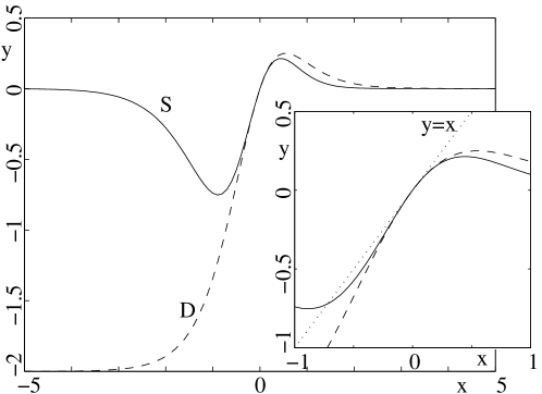
Figure 9: The dashed lines indicate the quantity $D$ (63) and the solid lines the quantity $S$ (64). If one has a particular distribution of sparse couplings $\phi$ then at the triple-point one can integrate over these distributions to determine the quantities and hence the nature of reentrant behaviour – whether the weakly ordered systems are dominated by dense or sparse type order, we find the former in canonical cases. If the variance of the distributions is sufficient the integral for both quantities is negative. If the distribution is of positive mean with low variance both quantities will be positive. It is possible to generate many distributions for which the above generalisations do not hold, and reentrant behaviour of an alternative type may occur.

Appendix D Population dynamics numerical implementation

The population dynamics is implemented such that the fields are assigned randomly at time $t=0$ in three histograms (real replica) simultaneously. We consider the development from initial conditions corresponding to frozen ferromagnetic, SG and near paramagnetic (high temperature) initial condition histograms. The corresponding Gaussian distributions are

$$P(h^{(0)}_{i}) = {\cal N}(1000,0)\qquad,\qquad{\cal N}(0,1)\qquad\mbox{and}\qquad{\cal N}(0,0.001)\;,$$ (65)

We also add an additional (fourth) histogram with ferromagnetic order along the dense alignment when ${\bar{b}}\neq 1$, and initialise $b_{i}^{(0)}$ to $\pm 1$ with probabilities determined by ${\bar{b}}$.

Since the representative low-temperature order parameters are overestimated in the former two, and underestimated in the latter, we can be confident a solution converged to by all three will not be systematically biased. However, in the case of multiple locally stable solutions these replica remain disparate, but cover a representative set of solutions quite well (e.g. ${\bar{b}}=0$). This parallelism is at the cost of runtime, but we found drift, or metastability, to be prevalent effects justifying the method.

It is also useful to consider fluctuations of the solutions within a single histogram in successive time steps ($N$ field updates). We judge convergence in both cases through consideration of the order parameters $q_{1}$, ${\bar{q}}_{1}$, and $q_{2}$. This is insufficient for a system involving sparse interactions since the distribution is then not Gaussian, but appears nevertheless to be quite robust and comparable to other heuristic methods attempted. The criteria for termination of the algorithm is that the distributions based on all 3 (4) initial conditions and between successive updates converges in $q_{1}$,${\bar{q}}_{1}$ and $q_{2}$ to within a worst case absolute precision of $0.01$. Finite size fluctuations and runtime constraints prevent a signigicantly stronger precision.

The field updates of (44) are random and non-sequential – but ensuring that in each time step, each field is updated exactly once.

We found in almost all cases that histograms converged to a single unique distribution (upto finite size errors), and that this convergence was robust. When convergence criteria is met we analyse the histogram (replica) of lowest free energy as representative. Measurables are determined following convergence based on 20 samples over 20 time steps. For certain systems we ran upto $20$ independent runs (different pseudo random update sequences) to check the properties were unique and fully explore the space.

In the case of non-convergence by the moments criteria we halt the algorithm after $500$ time steps and consider the histogram that corresponds to the lowest free energy (amongst the different initial condition histograms), calculating quantities based on this choice. In the case that metastable solutions exists this is sufficient to identify the histogram corresponding to a dominant state. This occured only for certain systems with opposite ferromagnetic alignment (${\bar{b}}=0$). In all other cases it appeared solutions are in the vicinity of the correct saddlepoint but converging with different bises; thus identifying the solution of lowest free energy does not guarantee improved measurement of the statistics in this case. However, we judge the statistics collected to be close in most cases.

D.1 Stability

We associate with each field in the population dynamics a perturbation $\delta h_{i}^{2}$, these are initially chosen with a Gaussian distribution independent of the field. With $\gamma>0$ convergence to a non-Gaussian joint distribution of perturbations and fields must be considered, we observed this to occur very quickly as can be determined in correlation functions and kurtosis, e.g. $\left\langle\delta(h_{i}^{t})^{2}(h_{i}^{t})^{2}\right\rangle_{C}$ and $\left\langle\delta h_{i}^{4}\right\rangle$, but could not produce a robust measure of convergence of the fluctuation distribution. Following convergence in the order parameters, we introduce the field and following $10$ time steps collect data over 20 time steps. Distribution of perturbations are carefully renormalised throughout analysis to account for the non-sequential updates, and the renormalisation after each time-step provides an estimate for $\chi_{2}$. Certain other numerical hacks must be brought to bear to prevent divergences in the cases where $\chi_{2}$ is not close to $0$.

References

References

- [BS07] Barra, A., and Sanctis, L. D., Stability properties and probability distribution of multi-overlaps in dilute spin glasses, J. Stat. Mech. (2007), P08025.
- [dAT78] de Almeida, J. R. L., and Thouless, D. J., Stability of the sherrington-kirkpatrick solution of a spin glass model, J. Phys. A 11 (1978), 983–990.
- [ER70] Erdös, P., and Re’nyi, A., On a new law of large numbers, J. Analyse Math. 23 (1970), 103–111.
- [GBM01] Giardina, I., Bouchaud, J., and M zard, M., Population dynamics in a random environment, J. Phys. A 34 (2001), L245–L252.
- [HM] Hase, M. O., and Mendes, J. F. F., Diluted antiferromagnet in a ferromagnetic environment, arXiv:0711.3016v1.
- [Kab03] Kabashima, Y., Propagating beliefs in spin glass models, J. Phys. Soc. Jpn. 72 (2003), 1645–1649.
- [Mat] Mattis, D. C., Solvable spin systems with random interactions, Phys. Lett. A 56.
- [Mon98] Monasson, R., Optimization problems and replica symmetry breaking in finite connectivity spin glasses, J. Phys. A 31 (1998), 513–529.
- [Mot87] Mottishaw, P., Replica symmetry breaking and the spin-glass on a bethe lattice, Europhys. Lett. 3 (1987), 333–337.
- [MPV87] Mézard, M., Parisi, G., and Virasoro, M., Spin glass theory and beyond, World Scientific Publishing Co., Singapore, 1987.
- [Nis01] Nishimori, H., Statistical physics of spin glasses and information processing, Oxford University Press, Oxford, UK, 2001.
- [Ost06] Ostilli, M., Ising spin glass models versus ising models: an effective mapping at high temperature: I. general result, Jour. of Stat. Phys. (2006), P10004.
- [Par] Parisi, G., Stochastic stability, arXiv:cond-mat/0007347.
- [RBMM04] Rivoire, O., Biroli, G., Martin, O. C., and M zard, M., Glass models on bethe lattices, Euro. Phys. J. B 37 (2004), 55–78.
- [RS07] Raymond, J., and Saad, D., Sparsely-spread cdma - a statistical mechanics based analysis, J. Phys. A 40 (2007), 12315–12333.
- [SK75] Sherrington, D., and Kirkpatrick, S., Solvable model of a spin-glasses, Phys. Rev. Lett. 35 (1975), 1792–1796.
- [Tal03] Talagrand, M., Spin glasses: A challenge for mathematicians: Cavity and mean field models, Springer, Berlin, Germany, 2003.
- [VB85] Viana, L., and Bray, A., Phase diagrams for dilute spin glasses, J. Phys. C 18 (1985), 3037–3051.
- [WS88] Wong, K., and Sherrington, D., Intensively connected spin glasses: towards a replica-symmetry-breaking solution of the groud state, J. Phys. A 21 (1988), L459–L466.