Imbalanced d-wave superfluids in the BCS-BEC crossover regime at finite temperatures.

Abstract

Singlet pairing in a Fermi superfluid is frustrated when the amounts of fermions of each pairing partner are unequal. The resulting ‘imbalanced superfluid’ has been realized experimentally for ultracold atomic gases with $s$-wave interactions. Inspired by high-temperature superconductivity, we investigate the case of $d$-wave interactions, and find marked differences from the $s$-wave superfluid. Whereas $s$-wave imbalanced Fermi gases tend to phase separate in real space, in a balanced condensate and an imbalanced normal halo, we show that the $d$-wave gas can phase separate in reciprocal space so that imbalance and superfluidity can coexist spatially. We show that the mechanism explaining this property is the creation of polarized excitations in the nodes of the gap. The Sarma mechanism, present only at nonzero temperatures for the $s$-wave case, is still applicable in the temperature zero limit for the $d$-wave case. As a result, the $d$-wave BCS superfluid is more robust with respect to imbalance, and a region of the phase diagram can be identified where the $s$-wave BCS superfluidity is suppressed whereas the $d$-wave superfluidity is not. When these results are extended into the BEC limit of strongly bound molecules, the symmetry of the order parameter matters less. The effects of fluctuations beyond mean field is taken into account in the calculation of the structure factor and the critical temperature. The poles of the structure factor (corresponding to bound molecular states) are less damped in the $d$-wave case as compared to $s$-wave. On the BCS side of the unitarity limit, the critical temperature $T_{c}$ follows the temperature $T^{\ast}$ corresponding to the pair binding energy and as such will also be more robust against imbalance. Possible routes for the experimental observation of the $d$-wave superfluidity have been discussed.

LABEL:FirstPage1 LABEL:LastPage#1

I Introduction

In a metal exhibiting superconductivity at low temperature, the amount of spin-up and spin-down electrons are equal, and the electron-phonon interaction leading to Cooper pairing has a given, fixed strength. Both the population of the spin-components and the electron-phonon interaction strength cannot be arbitrarily tuned, and this restricts the experimental study of superconductivity to some given values in parameter space. Nevertheless one would like to access a much larger region of parameter space to gain insight in pairing and the superconductivity.

Superfluid Fermi gases have recently gained a lot of interest, precisely because of the accurate adaptability of the system parameters. The interaction strength between the two hyperfine spin states is an adjustable parameter. This allows to probe pairing and superfluidity in the crossover between a Bardeen-Cooper-Schrieffer (BCS) state of weakly bound Cooper pairs and a Bose-Einstein condensate (BEC) of tightly bound molecules FermiBCS ; FermiBEC . Moreover, in a mixture of two hyperfine spin states of a fermionic element, the amount of each hyperfine spin component can be controlled experimentally. This permits to investigate the effect that a population imbalance between the spin components has on pairing MIT-imbal ; RICE-imbal . Not surprisingly, these recent experimental breakthroughs MIT-imbal ; RICE-imbal ; FermiBCS ; FermiBEC have relaunched the theoretical efforts to understand imbalanced Fermi superfluids in the crossover regime theory-imbal .

The first theoretical study of Cooper pairing in an imbalanced Fermi mixture was performed in the context of BCS superconductors by Clogston ClogstonPRL9 , who showed that a population imbalance destroys the superconductivity when the imbalance in chemical potentials is of the same order as the ‘balanced’ order parameter. Experiments confirm that imbalance frustrates pairing, and reveal that the excess spin component is preferentially expelled from the superfluid FermiBCS ; FermiBEC : demixing occurs DeSilvaPRA73 . More exotic pairing scenarios have been predicted, most notoriously the ‘Fulde-Ferrell-Larkin-Ovchinnikov’ scenario FFLO in which the Fermi spheres of the two components spontaneously deform, leading to Cooper pairs with nonzero center-of-mass momentum.

When the temperature is raised and excitations are populated, the superconductivity may be restored by creating a ‘balanced’ pair condensate with an ‘imbalanced’ gas of excitations. This may lead to ‘reentrant superconductivity’ as proposed by Sarma SarmaJPCS24 . In the Sarma state, the excess spin component is expelled from the superfluid, not in position space, but in energy space.

In the context of the Sarma state, the case of an imbalanced Fermi gas with a $d$-wave order parameter is particularly interesting. In the current experiments on superfluid Fermi gases, the temperatures are low enough so that only the $s$-wave partial wave matters, and the $d$-wave scattering is much weaker than the $s$-wave interactions. However, the $d$-wave order parameter has directions in momentum space where it vanishes, even at zero temperature. This allows for a Sarma scenario where the excess spin component is expelled from the superfluid, not in position or energy space, but in momentum space. In this contribution, we show that $d$-wave symmetry enables the superfluid to cope with imbalance all the way to temperature zero, using a similar scenario as proposed by Sarma for nonzero temperature. This leads to the conclusion that imbalance can stabilize the $d$-wave pairs with respect to the $s$-wave pairs since the $d$-wave superfluid is more robust against population imbalance. Moreover, since also the $d$-wave scattering length can be tuned through the Feshbach mechanism, we investigate the $d$-wave superfluidity both in BEC and BCS regimes.

The case of the $d$-wave pairing in the BEC/BCS crossover is also interesting from the point of view of high-temperature superconductivityranderia , where the order parameter is found to exhibit $d$-wave symmetrywisenature . The current results, derived in the context of cold atomic gases, can also shed light on properties of the pseudogap state in the underdoped regime. This pseudogap (which appears to have the same $d$-wave symmetry as the order parameterWilliamsPRL87 ) has been associated either with some competing order parameter in the normal state, or with the existence of ”pre-formed pairs”,alexandrovbook where a notable candidate is the non-condensed bipolaronalexandrov . Also in the current treatment, pre-formed $d$-wave pairs appear, and we present results for the pair binding energy of these objects as a function of temperature, density and interatomic interaction strength.

Our formalism of choice to treat the imbalanced Fermi gases is path-integration. The path-integral formalism was effectively applied to study fermionic superfluidity in dilute gases using the approach with the Hubbard-Stratonovic transformation, choosing a saddle point, and performing the integration over the fermionic variables. This leaves an effective action depending on the saddle point value and the chemical potential. The effective action can be applied to study the Fermi superfluid in optical lattices ourlattice or to investigate vortices in Fermi superfluids ourvortex . In Ref. demelo1993 , that approach was extended in order to take into account the fluctuations around the saddle point. The treatment starts from the partition function, which is the path integral over fermionic (Grassmann) variables. After the introducing the auxiliary bosonic variables and integrating over the fermionic variables, the exact expression for the partition function from demelo1993 is the path integral over only the boson fields with an effective bosonic action. That action is then represented as a sum of the saddle-point contribution (which is calculated exactly) and the contribution due to Gaussian fluctuations, which is taken into account as a perturbation. At $T=T_{c}$, this approximation for the fluctuations is equivalent to that of Nozières and Schmitt-Rink NSR .

The further development of this idea can be found, e. g., in Refs. Taylor2006 ; Randeria2007 . In Ref. Taylor2006 , the superfluid density is derived for a uniform two-component Fermi gas in the BCS-BEC crossover regime in the presence of an imposed superfluid flow, taking into account pairing fluctuations in a Gaussian approximation following Ref. NSR . In Refs. Engelbrecht1997 ; Randeria2007 , the effects of quantum fluctuations about the saddle-point solution of the BCS-BEC crossover at $T=0$ in a dilute Fermi gas are included at the Gaussian level using the functional integral method. In Ref. Fukushima2007 , the superfluid density and the condensate fraction are investigated for a fermion gas in the BCS-BEC crossover regime at finite temperatures. The fluctuation effects on these quantities are included within a Gaussian approximation. The gas of interacting fermions in Refs. Taylor2006 ; Randeria2007 ; Fukushima2007 is considered for the $s$-wave pairing and with no population imbalance. A study of the balanced $d$-wave system using the path-integral method can be found in Ref. DM2000 . Finally, the current work applies the path-integral theory to the imbalanced $d$-wave superfluids, including finite-temperature fluctuations, to show that $d$-wave pairing is particularly robust against imbalance fluctuations.

The formalism is presented in Section II. In Section III, we develop the mean-field approach and discuss the resulting pair binding energy. In Section IV, we also include the fluctuations to treat the finite-temperature case and determine the critical temperature for superfluidity. Near the unitarity limit where mean-field is known to fail it is necessary to include fluctuations, but also to incorporate the normal-state interactions in the description. The current approach achieves this through an expansion of the action around the saddle point that keeps terms related to the particle-hole excitations. To investigate these excitations, we calculate in Section V the structure factor for the $d$-wave and compare it to the structure factor in the $s$-wave pairing state.

II Formalism

II.1 $d$-wave interactions

As in Refs. demelo1993 ; Randeria2007 , we start by writing down the partition function of the interacting Fermi gas as a path integral over Grassmann variables:

$$\mathcal{Z}\propto\int\mathcal{D}\bar{\psi}_{\mathbf{k},n,\sigma}\mathcal{D}\psi_{\mathbf{k},n,\sigma}\exp\left(-S\right)$$ (1)

Rather than use position and imaginary time variable, we have Grassmann fields $\bar{\psi}_{\mathbf{k},n,\sigma}$,$\psi_{\mathbf{k},n,\sigma}$ that depend on the wave number $\mathbf{k}$ and the fermionic Matsubara frequency $\omega_{n}=n\pi/\beta$ with $n$ an odd integer and $\beta=1/(k_{B}T)$ the inverse temperature. Two different hyperfine spin states are trapped so that we include a spin quantum number $\sigma$ in the description. We’ll denote the two states as ’spin-up’, $\sigma=\uparrow$ and ’spin down’, $\sigma=\downarrow$.

The action functional $S=S_{0}+S_{I}$ consists of a ’non-interacting part’, $S_{0}$, and the interaction terms, $S_{I}$. The former is given by

$$S_{0}=\sum_{\mathbf{k},n}\sum_{\sigma}\left(-i\omega_{n}+k^{2}-\mu_{\sigma}\right)\bar{\psi}_{\mathbf{k},n,\sigma}\psi_{\mathbf{k},n,\sigma}$$ (2)

where $\mu_{\sigma}$ is the chemical potential fixing the amount of atoms of species $\sigma$, and where the summations run over all possible indices of the Grassmann variables. We use units such that $\hbar=k_{F}=2m_{f}=1$, where $m_{f}$ is the mass of the fermionic atoms, and $k_{F}$ is the Fermi wave vector of the non-interacting, balanced Fermi gas with the same total number of particles. In what follows, we will use the average chemical potential $\mu=(\mu_{\uparrow}+\mu_{\downarrow})/2$ along with the difference in chemical potentials $\zeta=(\mu_{\uparrow}-\mu_{\downarrow})/2$, rather than the chemical potentials of the individual species.

The interaction terms of the action functional are written in a form that emphasizes the pairs of colliding fermions:

$$S_{I}=\sum_{\mathbf{q},m}\sum_{\mathbf{k},n}\sum_{\mathbf{k}^{\prime},n^{\prime}}\text{ }V_{pp}\left(\mathbf{k,k}^{\prime}\right)\bar{\psi}_{\frac{\mathbf{q}}{2}+\mathbf{k},\frac{m}{2}+n,\uparrow}\bar{\psi}_{\frac{\mathbf{q}}{2}-\mathbf{k},\frac{m}{2}-n,\downarrow}\psi_{\frac{\mathbf{q}}{2}-\mathbf{k}^{\prime},\frac{m}{2}-n^{\prime},\downarrow}\psi_{\frac{\mathbf{q}}{2}+\mathbf{k}^{\prime},\frac{m}{2}+n^{\prime},\uparrow}$$ (3)

Here $V_{pp}$ is the interaction potential. The wave numbers in this collision term are written as the sum of a center-of-mass wave number $\mathbf{q}$ and the relative wave numbers $\mathbf{k,k}^{\prime}$ before and after collision. Similarly, the Matsubara frequencies are decomposed in a center-of-mass bosonic frequency $\Omega_{m}=2m\pi/\beta$ and relative fermionic frequencies $\omega_{n},\omega_{n^{\prime}}$. Here, we consider only interactions that couple fermions from different hyperfine spin states. We’ll need a further assumption on the interaction potential to proceed. As in DM2000 ; demelopwave we assume that the interatomic interaction potential can factorized as

$$V_{pp}\left(\mathbf{k,k}^{\prime}\right)=g\Gamma\left(\mathbf{k}\right)\Gamma\left(\mathbf{k}^{\prime}\right)$$ (4)

This is possible for $s$-wave pairing

$$g=g_{s},\;\Gamma_{s}\left(\mathbf{k}\right)=1,$$ (5)

and also for $d$-wave pairing

$$g=g_{d},\;\Gamma_{d}\left(\mathbf{k}\right)=\frac{\left(k/k_{1}\right)^{2}}{\left(1+k/k_{0}\right)^{5/2}}\sqrt{\frac{28\pi}{15}}Y_{2,0}\left(\theta,\varphi\right).$$ (6)

Here, $Y_{2,0}\left(\theta,\varphi\right)$ is the spherical harmonic, and $k_{1},k_{0}$ are parameters fixing the range of the potential. The constant $g<0$ ($g>0$) corresponds to attraction (repulsion). These constants can be related to the $s$-and $d$-wave scattering lengthsizdiasz . The usefulness of the factorization (4) lies in the fact that it allows to rewrite the interaction terms as

$$S_{I}=g\sum_{\mathbf{q},m}\bar{A}_{\mathbf{q},m}A_{\mathbf{q},m}$$ (7)

where we introduced the collective fields

$$A_{\mathbf{q},m} =\sum_{n,\mathbf{k}}\frac{\Gamma\left(\mathbf{k}\right)}{\sqrt{\beta V}}\psi_{\frac{\mathbf{q}}{2}-\mathbf{k},\frac{m}{2}-n,\downarrow}\psi_{\frac{\mathbf{q}}{2}+\mathbf{k},\frac{m}{2}+n,\uparrow},$$

$$\bar{A}_{\mathbf{q},m} =\sum_{n,\mathbf{k}}\frac{\Gamma\left(\mathbf{k}\right)}{\sqrt{\beta V}}\bar{\psi}_{\frac{\mathbf{q}}{2}+\mathbf{k},\frac{m}{2}+n,\uparrow}\bar{\psi}_{\frac{\mathbf{q}}{2}-\mathbf{k},\frac{m}{2}-n,\downarrow}.$$ (8)

Here $V$ is the system volume. The Hubbard-Stratonovic transformation can transform the product over these collective fields into a sum over them, at the expense of introducing an additional functional integration:

$$\mathcal{Z}\propto\int\mathcal{D}\bar{\psi}_{\mathbf{x},\tau,\sigma}\mathcal{D}\psi_{\mathbf{x},\tau,\sigma}\int\mathcal{D}\bar{\Delta}_{\mathbf{q},m}\mathcal{D}\Delta_{\mathbf{q},m}\exp\left(-S\right)$$ (9)

with the action

$$S =\sum_{\mathbf{k},n,\sigma}\left(-i\omega_{n}+k^{2}-\mu_{\sigma}\right)\bar{\psi}_{\mathbf{k},n,\sigma}\psi_{\mathbf{k},n,\sigma}$$ (10)

$$-\sum_{m,\mathbf{q}}\left(\frac{\bar{\Delta}_{\mathbf{q},m}\Delta_{\mathbf{q},m}}{g}+\bar{\Delta}_{\mathbf{q},m}A_{\mathbf{q},m}+\Delta_{\mathbf{q},m}\bar{A}_{\mathbf{q},m}\right).$$ (11)

Note that the auxiliary fields $\bar{\Delta}_{\mathbf{q},m},\Delta_{\mathbf{q},m}$ are bosonic in nature, and characterized by the center-of-mass pair wave number and bosonic Matsubara frequency $\Omega_{m}=2m\pi/\beta$. The decoupling of the collective fields is necessary to perform the functional integral over Grassmann variables, resulting in

$$\mathcal{Z}\propto\int\mathcal{D}\bar{\Delta}_{\mathbf{q},m}\mathcal{D}\Delta_{\mathbf{q},m}\exp\left(\mathtt{tr}\ln\left[\mathbb{G}^{-1}\left(\mathbf{q},m;\mathbf{k},n\right)\right]+\frac{1}{g}\sum_{m,\mathbf{q}}\bar{\Delta}_{\mathbf{q},m}\Delta_{\mathbf{q},m}\right),$$ (12)

where $-\mathbb{G}^{-1}$ is the inverse Nambu tensor and the trace has to be taken over the fermionic degrees of freedom.

The value where the (exponential) integrand becomes largest is called the saddle point. Interpreting $\Delta_{\mathbf{q},m}$ as the field of bosonic pairs, we can claim that when these pairs are condensed, the largest contribution derives from the terms with $\Delta_{\mathbf{0},0}=\Delta$. Performing the Bogoliubov shift, we change integration variables from $\Delta_{\mathbf{q},m}$ to $\gamma_{\mathbf{q},m}$ where

$$\bar{\Delta}_{\mathbf{q},m} =\sqrt{V\beta}\Delta\delta_{m,0}\delta_{\mathbf{q},0}+\gamma_{\mathbf{q},m},$$ (13)

$$\bar{\Delta}_{\mathbf{q},m} =\sqrt{V\beta}\bar{\Delta}\delta_{m,0}\delta_{\mathbf{q},0}+\bar{\gamma}_{\mathbf{q},m}.$$ (14)

If, at this point, we choose the saddle point not as the $q=0$ state, but as a state with a finite wave number, equal to the difference between the Fermi wave numbers of each component, we obtain the FFLO state FFLO . Since this has not yet been observed, we restrict the current calculations to $\mathbf{q}=0$ pairs. This allows to split up the inverse Nambu tensor

$$-\mathbb{G}^{-1}\left(\mathbf{q},m;\mathbf{k},n\right)=\delta_{m,0}\delta_{\mathbf{q},0}\left[-\mathbb{G}_{sp}^{-1}\left(\mathbf{k},n\right)\right]+\mathbb{F}\left(\mathbf{q},m;\mathbf{k}\right),$$ (15)

with the saddle-point contribution is

$$-\mathbb{G}_{sp}^{-1}\left(\mathbf{k},n\right)=\left(\begin{array}[c]{cc}-i\omega_{n}+k^{2}-\mu_{\uparrow}&-\Gamma\left(\mathbf{k}\right)\Delta\\ -\Gamma\left(\mathbf{k}\right)\bar{\Delta}&-i\omega_{n}-k^{2}+\mu_{\downarrow}\end{array}\right)$$ (16)

and the fluctuation contribution is

$$\mathbb{F}\left(\mathbf{q},m;\mathbf{k}\right)=\frac{\Gamma\left(\mathbf{k}\right)}{\sqrt{\beta V}}\left(\begin{array}[c]{cc}0&-\gamma_{\mathbf{q},m}\\ -\bar{\gamma}_{-\mathbf{q},-m}&0\end{array}\right).$$ (17)

We are left with the functional integration over the bosonic fields $\gamma_{\mathbf{q},m}$ and $\bar{\gamma}_{\mathbf{q},m}$. The simplest approximation consists in ignoring these fluctuations and setting $\mathbb{G}=\mathbb{G}_{sp}$ – this yields the saddle point results and will be explored in the next subsection, III.B. Expanding $\ln\left[\mathbb{G}^{-1}\right]$ in successive orders of $\mathbb{F}$ yields a perturbation series in $\gamma_{\mathbf{q},m}$ corresponding to an ever increasing diagrammatic expansion, with possible Dyson resummations. The term of order $\mathbb{F}^{2}$ is still quadratic and we calculate it in subsection III.C. Up to second order:

$$\mathcal{Z}\propto\exp\left\{-S_{sp}\right\}\times\int\mathcal{D}\bar{\gamma}_{\mathbf{q},m}\mathcal{D}\gamma_{\mathbf{q},m}\exp\left\{-S_{fl}\right\}$$ (18)

with

$$S_{sp}=\mathtt{tr}\ln\left[\mathbb{G}_{sp}^{-1}\right]-\frac{V\beta}{g}\bar{\Delta}\Delta$$ (19)

and

$$S_{fl}=\frac{1}{2}\operatorname*{tr}\left(\mathbb{G}_{sp}\mathbb{FG}_{sp}\mathbb{F}\right)-\frac{1}{g}\sum_{\mathbf{q},m}\bar{\gamma}_{\mathbf{q},m}\gamma_{\mathbf{q},m}.$$ (20)

Since the partition sum is a product $\mathcal{Z}=\mathcal{Z}_{sp}\times\mathcal{Z}_{fl}$ , the corresponding thermodynamic potential will be a sum of a saddle-point contribution and fluctuations: $F=F_{sp}+F_{fl}$. The contributions are defined by $\mathcal{Z}=e^{-\beta F}$ and $\mathcal{Z}_{sp,fl}=e^{-\beta F_{sp,fl}}$. These thermodynamic potentials will be necessary to calculate the two number equations in subsection III.D.

II.2 Saddle-point action

The trace over $\mathbb{G}_{sp}^{-1}\left(\mathbf{k},n\right)$ can be performed, yielding

$$\mathcal{Z}_{sp}=\exp\left(-S_{sp}\right)=\exp\left(-\beta F_{sp}\right)$$

with $S_{sp}$ the saddle-point action

$$S_{sp}=-\sum_{\mathbf{k},n}\ln\left[\left(i\omega_{n}-\zeta-E_{\mathbf{k}}\right)\left(-i\omega_{n}+\zeta-E_{\mathbf{k}}\right)\right]-\frac{\beta V}{g}\bar{\Delta}\Delta.$$ (21)

where the reader is reminded that $\zeta=(\mu_{\downarrow}-\mu_{\uparrow})/2$ is the difference in chemical potentials. The Bogoliubov energy is

$$E_{\mathbf{k}}=\sqrt{\left(k^{2}-\mu\right)^{2}+\left|\Gamma\left(\mathbf{k}\right)\Delta\right|^{2}}.$$ (22)

The sum over fermionic Matsubara frequencies can be calculated. We find for $F_{sp}$, the saddle-point thermodynamic potential per unit volume,

$$\frac{F_{sp}}{V}=-\int\frac{d\mathbf{k}}{\left(2\pi\right)^{3}}\left[\frac{1}{\beta}\ln\left(2\cosh\beta\zeta+2\cosh\beta E_{\mathbf{k}}\right)-\xi_{\mathbf{k}}\right]-\frac{1}{g}\left|\Delta\right|^{2}.$$ (23)

where the fermion energy is $\xi_{\mathbf{k}}=k^{2}-\mu.$ Thus, the saddle-point result is generic for all interaction potentials of the form (4).

II.3 Quadratic fluctuations

When the terms of order $\mathcal{O}\left(\mathbb{F}^{3}\right)$ and higher are neglected in $S_{fl}$, the functional integral over $\bar{\gamma}_{\mathbf{q},m},\gamma_{\mathbf{q},m}$ in expression (18) can be performed. The result is written as

$$S_{fl}=\frac{F_{fl}}{\beta V}=\frac{1}{2}\int\frac{d\mathbf{q}}{\left(2\pi\right)^{3}}\sum_{m}\ln\left[\left|\mathcal{M}_{1,1}\left(\mathbf{q},i\Omega_{m}\right)\right|^{2}-\left|\mathcal{M}_{1,2}\left(\mathbf{q},i\Omega_{m}\right)\right|^{2}\right]$$ (24)

where now the trace is to be taken over bosonic Matsubara frequencies and center of mass wave numbers. Here,

$$\mathcal{M}_{1,1}\left(\mathbf{q},i\Omega_{n}\right) =\int\frac{d\mathbf{k}}{\left(2\pi\right)^{3}}\Gamma^{2}\left(\mathbf{k}\right)\left[\frac{1}{2k^{2}}+\frac{\sinh\beta E_{\mathbf{k}-\frac{\mathbf{q}}{2}}}{2E_{\mathbf{k}-\frac{\mathbf{q}}{2}}\left(\cosh\beta E_{\mathbf{k}-\frac{\mathbf{q}}{2}}+\cosh\beta\zeta\right)}\right.$$

$$\times\left(\frac{\left(i\Omega_{n}-E_{\mathbf{k}-\frac{\mathbf{q}}{2}}+\xi_{\mathbf{k}+\frac{\mathbf{q}}{2}}\right)\left(E_{\mathbf{k}-\frac{\mathbf{q}}{2}}+\xi_{\mathbf{k}-\frac{\mathbf{q}}{2}}\right)}{\left(i\Omega_{n}-E_{\mathbf{k}-\frac{\mathbf{q}}{2}}+E_{\mathbf{k}+\frac{\mathbf{q}}{2}}\right)\left(i\Omega_{n}-E_{\mathbf{k}-\frac{\mathbf{q}}{2}}-E_{\mathbf{k}+\frac{\mathbf{q}}{2}}\right)}\right.$$

$$\left.\left.-\frac{\left(i\Omega_{n}+E_{\mathbf{k}-\frac{\mathbf{q}}{2}}+\xi_{\mathbf{k}+\frac{\mathbf{q}}{2}}\right)\left(E_{\mathbf{k}-\frac{\mathbf{q}}{2}}-\xi_{\mathbf{k}-\frac{\mathbf{q}}{2}}\right)}{\left(i\Omega_{n}+E_{\mathbf{k}-\frac{\mathbf{q}}{2}}-E_{\mathbf{k}+\frac{\mathbf{q}}{2}}\right)\left(i\Omega_{n}+E_{\mathbf{k}+\frac{\mathbf{q}}{2}}+E_{\mathbf{k}-\frac{\mathbf{q}}{2}}\right)}\right)\right]-\lambda\left(a\right),$$ (25)

with the parameters $\lambda\left(a\right)$ which describe the coupling strength for the $s$-wave and $d$-wave pairingsizdiasz :

$$\lambda_{s}\left(a_{s}\right)=\frac{1}{8\pi a_{s}},\;\lambda_{d}\left(a_{d}\right)=\frac{2}{\pi a_{d}^{5}},$$ (26)

and

$$\mathcal{M}_{1,2}\left(\mathbf{q},i\Omega_{n}\right) =-\left|\Delta\right|^{2}\int\frac{d\mathbf{q}}{\left(2\pi\right)^{3}}\Gamma^{2}\left(\mathbf{k}\right)\Gamma\left(\mathbf{k}+\frac{\mathbf{q}}{2}\right)\Gamma\left(\mathbf{k}-\frac{\mathbf{q}}{2}\right)$$

$$\times\frac{\sinh\beta E_{\mathbf{k}-\frac{\mathbf{q}}{2}}}{2E_{\mathbf{k}-\frac{\mathbf{q}}{2}}\left(\cosh\beta E_{\mathbf{k}-\frac{\mathbf{q}}{2}}+\cosh\beta\zeta\right)}$$

$$\times\left(\frac{1}{\left(i\Omega_{n}-E_{\mathbf{k}-\frac{\mathbf{q}}{2}}+E_{\mathbf{k}+\frac{\mathbf{q}}{2}}\right)\left(i\Omega_{n}-E_{\mathbf{k}-\frac{\mathbf{q}}{2}}-E_{\mathbf{k}+\frac{\mathbf{q}}{2}}\right)}\right.$$

$$\left.+\frac{1}{\left(i\Omega_{n}+E_{\mathbf{k}-\frac{\mathbf{q}}{2}}-E_{\mathbf{k}+\frac{\mathbf{q}}{2}}\right)\left(i\Omega_{n}+E_{\mathbf{k}-\frac{\mathbf{q}}{2}}+E_{\mathbf{k}+\frac{\mathbf{q}}{2}}\right)}\right).$$ (27)

In the particular case of the $s$-wave pairing and of the balanced fermion gas, (25) and (27) are equivalent to the matrix elements derived in Ref. Engelbrecht1997 . In the present treatment, as distinct from Refs. Engelbrecht1997 ; Randeria2007 , we do not assume the low-temperature limit.

II.4 Gap and number equations

The gap equation is determined by $S_{sp}$ alone, through $\delta S_{sp}/\delta\Delta=0$. The gap equation can be written in a unified form for the $s$-wave and $d$-wave pairings,

$$\int\frac{d\mathbf{k}}{\left(2\pi\right)^{3}}\left|\Gamma\left(\mathbf{k}\right)\right|^{2}\left(\frac{\sinh\beta E_{\mathbf{k}}}{2E_{\mathbf{k}}\left(\cosh\beta E_{\mathbf{k}}+\cosh\beta\zeta\right)}-\frac{1}{2k^{2}}\right)+\lambda\left(a\right)=0.$$ (28)

The number equations are determined from the thermodynamic potential through

$$\left(\frac{\partial F}{\partial\mu}\right)_{T,V,\Delta} =-n,$$ (29)

$$\left(\frac{\partial F}{\partial\zeta}\right)_{T,V,\Delta} =-\delta n,$$ (30)

where $n=n_{\uparrow}+n_{\uparrow}$ is the total local density, and $\delta n=n_{\uparrow}-n_{\uparrow}$ is the local population imbalance. For a finite temperature below $T_{c}$, the chemical potentials $\mu$ and $\zeta$, and the gap $\Delta$ are determined self-consistently as a solution of the gap equation (28) coupled with the number equations (29) and (30). In principle, we can write the exact thermodynamic potential $F=F_{sp}+F_{fl}+F_{other}$ where $F_{sp}$ and $F_{fl}$ are given by expressions (23) and (24), and $F_{other}$ comes from the contributions of all higher order terms, $\mathcal{O}\left(\mathbb{F}^{3}\right),$ in the exact action. The local density and the local population imbalance can be written as a sum of several contributions,

$$n =n_{sp}+n_{fl}+n_{other},$$ (31)

$$\delta n =\delta n_{sp}+\delta n_{fl}+\delta n_{other},$$ (32)

where $n_{sp}$ and $\delta n_{sp}$ are the saddle-point results, $n_{fl}$ and $\delta n_{fl}$ are the fluctuation contributions, and $n_{other}$, $\delta n_{other}$ are higher-order fluctuation contributions to the density and population imbalance, which are neglected in the present treatment.

The saddle-point contributions to the density and to the population imbalance are obtained using the saddle-point term of the thermodynamic potential (23) and Eqs. (29) and (30):

$$n_{sp} =\frac{1}{2\pi^{2}}\int_{0}^{\infty}k^{2}dk\left(1-\frac{\varepsilon_{\mathbf{k}}}{E_{\mathbf{k}}}\frac{\sinh\left(\beta E_{\mathbf{k}}\right)}{\cosh\left(\beta\zeta\right)+\cosh\left(\beta E_{\mathbf{k}}\right)}\right),$$ (33)

$$\delta n_{sp} =\frac{1}{2\pi^{2}}\int_{0}^{\infty}k^{2}dk\frac{\sinh\left(\beta\zeta\right)}{\cosh\left(\beta\zeta\right)+\cosh\left(\beta E_{\mathbf{k}}\right)}.$$ (34)

The fluctuation contribution to the number equations is determined on the basis of the fluctuation contribution to the thermodynamic potential:

$$n_{fl} =-\frac{1}{\beta}\int\frac{d\mathbf{q}}{\left(2\pi\right)^{3}}\sum_{n=-\infty}^{\infty}J\left(\mathbf{q},i\Omega_{n}\right),$$ (35)

$$\delta n_{fl} =-\frac{1}{\beta}\int\frac{d\mathbf{q}}{\left(2\pi\right)^{3}}\sum_{n=-\infty}^{\infty}K\left(\mathbf{q},i\Omega_{n}\right),$$ (36)

where the functions $J\left(\mathbf{q},z\right)$ and $K\left(\mathbf{q},z\right)$ for a complex argument $z$ are given by

$$J\left(\mathbf{q},z\right) =\frac{1}{\Gamma\left(\mathbf{q},z\right)}\left[\mathcal{M}_{1,1}\left(\mathbf{q},-z\right)\frac{\partial\mathcal{M}_{1,1}\left(\mathbf{q},z\right)}{\partial\mu}-\mathcal{M}_{1,2}\left(\mathbf{q},-z\right)\frac{\partial\mathcal{M}_{1,2}\left(\mathbf{q},z\right)}{\partial\mu}\right],$$ (37)

$$K\left(\mathbf{q},z\right) =\frac{1}{\Gamma\left(\mathbf{q},z\right)}\left[\mathcal{M}_{1,1}\left(\mathbf{q},-z\right)\frac{\partial\mathcal{M}_{1,1}\left(\mathbf{q},z\right)}{\partial\zeta}-\mathcal{M}_{1,2}\left(\mathbf{q},-z\right)\frac{\partial\mathcal{M}_{1,2}\left(\mathbf{q},z\right)}{\partial\zeta}\right],$$ (38)

with

$$\Gamma\left(\mathbf{q},z\right)=\mathcal{M}_{1,1}\left(\mathbf{q},z\right)\mathcal{M}_{1,1}\left(\mathbf{q},-z\right)-\mathcal{M}_{1,2}\left(\mathbf{q},z\right)\mathcal{M}_{1,2}\left(\mathbf{q},-z\right).$$ (39)

The functions $\mathcal{M}_{1,1}\left(\mathbf{q},z\right)$ and $\mathcal{M}_{1,2}\left(\mathbf{q},z\right)$ of the complex argument $z$ are analytical in the complex $z$-plane except the branching line, which lies at the real axis $z=\omega$. Similarly to Refs. demelo1993 ; Nozieres1985 , the summations over the boson Matsubara frequencies in (35) and (36) are converted to the contour integrals in the complex plane as described in the Appendix. Here, we write down the final result for the fluctuation contributions to $n$ and $\delta n$:

$$n_{fl} =-\int\frac{d\mathbf{q}}{\left(2\pi\right)^{3}}\left(\frac{1}{\pi}\int_{-\infty}^{\infty}\operatorname{Im}\left[\frac{J\left(\mathbf{q},\omega+i\gamma\right)}{e^{\beta\left(\omega+i\gamma\right)}-1}\right]d\omega+\frac{1}{\beta}\sum_{n=-n_{0}}^{n_{0}}J\left(\mathbf{q},i\Omega_{n}\right)\right),$$ (40)

$$\delta n_{fl} =-\int\frac{d\mathbf{q}}{\left(2\pi\right)^{3}}\left(\frac{1}{\pi}\int_{-\infty}^{\infty}\operatorname{Im}\left[\frac{K\left(\mathbf{q},\omega+i\gamma\right)}{e^{\beta\left(\omega+i\gamma\right)}-1}\right]d\omega+\frac{1}{\beta}\sum_{n=-n_{0}}^{n_{0}}K\left(\mathbf{q},i\Omega_{n}\right)\right).$$ (41)

Here, the number $n_{0}$ is chosen arbitrarily, and the parameter $\gamma$ lies in the range $\Omega_{n_{0}}<\gamma<\Omega_{n_{0}+1}$.

In particular, if one chooses $n_{0}=0,$ the formula (53) leads to the expression for the fluctuation contribution to the fermion density similar to that derived in Ref. demelo1993 :

$$n_{fl}=\frac{1}{\pi}\int\frac{d\mathbf{q}}{\left(2\pi\right)^{3}q^{2}}\int_{-\infty}^{\infty}d\omega S\left(\mathbf{q},\omega\right).$$ (42)

Here, the structure factor is

$$S\left(\mathbf{q},\omega\right)=-\frac{q^{2}\operatorname{Im}\left[J\left(\mathbf{q},\omega+i\delta\right)\right]}{e^{\beta\omega}-1},\;\delta\rightarrow+0.$$ (43)

The results obtained in the present section extends the path-integral approach of Ref. Randeria2007 to the case of the $d$-wave pairing and of an imbalanced Fermi gas at arbitrary temperatures. In agreement with the proof made in Ref. Nozieres1985 , the function

$$Q\left(\mathbf{q},\omega\right)\equiv\lim_{\delta\rightarrow+0}\left\{\operatorname{Im}\left[J\left(\mathbf{q},\omega+i\delta\right)\right]\right\}$$ (44)

at $T=T_{c}$ is equal to zero at $\omega=0$. Furthermore, $Q\left(\mathbf{q},\omega\right)$ changes its sign as $\omega$ passes through $\omega=0$. This is necessary to ensure that the relative contribution to the fluctuation density from excitations with given $\left(\mathbf{q},\omega\right)$ remains positive; this contribution is proportional to $S\left(\mathbf{q},\omega\right)$.

III Robustness of the $d$-wave pair binding energy

First we look at the saddle-point results for temperature zero, in order to investigate the pair binding energy. In the limit of temperature zero $\beta\rightarrow\infty$, the gap equation becomes

$$-\frac{2}{\pi(k_{F}a_{d})^{5}}=\int\frac{d\mathbf{k}}{(2\pi)^{3}}\left\{\frac{\Theta(E_{\mathbf{k}}>\zeta)}{2E_{\mathbf{k}}}-\frac{1}{2k^{2}}\right\}|\Gamma(\mathbf{k})|^{2}$$ (45)

with $\Theta$ the logical Heaviside function. Simultaneously the two saddle-point number equations (33),(34) become

$$\frac{1}{3\pi^{2}} =\int\frac{d\mathbf{k}}{(2\pi)^{3}}\left\{1-\Theta(E_{\mathbf{k}}>\zeta)\frac{\varepsilon_{\mathbf{k}}}{E_{\mathbf{k}}}\right\}$$ (46)

$$\frac{1}{3\pi^{2}}\frac{\delta n}{n} =\int\frac{d\mathbf{k}}{(2\pi)^{3}}\Theta(E_{\mathbf{k}}<\zeta).$$ (47)

The $\Theta(E_{\mathbf{k}}<\zeta)$ function cuts off all the wave numbers with energy less than $\zeta$. These are shown in Fig. 1. Near $\{k_{x},k_{y}\}=\{\sqrt{2},\sqrt{2}\}k_{F}$ the gap vanishes, and excitations are always present. To have non-zero imbalance in an $s$-wave superfluid, $\zeta$ has to be of the order of $\left|\Delta\right|$. This is the Clogston limit, and superfluidity will break down. However, for the $d$-wave superfluid all values of $\zeta$ lead to imbalance, and small values of $\zeta$ do not destroy superfluidity.

Figure 1: Even a small difference between the chemical potential leads to population imbalance. This plot shows the contours of $E_{\mathbf{k}}=\zeta$ for different values of $\zeta$ in the $k_{x},k_{y}$ plane, for a $d$-wave interaction characterized by $k_{0}=k_{1}=10k_{F}$. Within the regions $E_{\mathbf{k}}<\zeta$, spin-polarized Bogoliubov excitations are present that carry the excess spin component of the imbalanced gas.

Solving for a given imbalance and interaction strength $a_{d}$ the saddle-point number and gap equations (45)-(47), we can derive the saddle-point value $\Delta$. This value is necessary to compute the fluctuation effects, but it has an interpretation by itself, namely as the pair binding energy. A corresponding temperature $T^{\ast}=\left|\Delta\right|/k_{B}$ can be associated with the pair binding energy. In the BCS limit, superfluidity is destroyed by breaking up Cooper pairs. Thus, the transition temperature is determined by the binding energy of the Cooper pairs and $T_{c}\approx T^{\ast}$. However, in the BEC limit, superfluidity is destroyed not by breaking up the bosonic molecules, but by phase fluctuations, and typically $T_{c}\ll T^{\ast}$. The BEC limit, with its tightly bound molecules, is relatively insensitive to the addition of atoms of one of the spin species: the imbalanced system can be described as a mixture of fermionic atoms and bosonic molecules. The BCS limit, however, is very sensitive to imbalance. Since in the BCS limit $T_{c}$ is directly related to the pair binding energy $\left|\Delta\right|$, we gain insight in the effect of imbalance on $s$- and $d$-wave superfluids through the saddle-point gap.

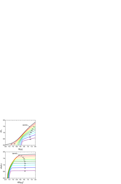
Figure 2: (color online) The dependence of the pair binding energy on the interaction strength for the $s$-wave (top) and $d$-wave (bottom) interaction is influenced by the imbalance $\delta n/n=0.0$ … $0.9$. On the BCS side, the imbalance destroys $s$-wave Cooper pairs for all values of $a_{s}<0$, but fails to break up the $d$-wave Cooper pairs.

The result for $\left|\Delta\right|$ is shown in Fig. 2 for $s$-wave (top panel) and $d$-wave (bottom panel) pairing. There are some notable differences between $s$- and $d$-wave results. Firstly, for the $d$-wave interaction the $x$-axis is a function of $1/(k_{F}a_{d})^{5}$ in stead of  $1/(k_{F}a_{s})$. This means that the $d$-wave scattering length should be much closer to resonance as compared to the $s$-wave case before superfluidity enters the resonant regime. The absolute scale still depends on $k_{0}$, related to the range of the interaction potential. Also the scale of the y-axis in the graph (representing $\left|\Delta\right|)$ has this dependence on the details of the potential embodied in $\Gamma(\mathbf{k})$.

A second difference between $s$- and $d$-wave resonant pairing, is that for $s$-wave interactions we find that there is pairing for all values of $a_{s}<0$. For $d$-wave interactions, it is no longer true that for any attractive potential there is pairing. There needs to be a fatal attraction before pairing occurs on the BCS side. The BEC side, however, is more or less the same for $s$- and $d$-wave. Deep in the BEC regime it indeed should not matter whether we have $s$-wave or $d$-wave internal parameter.

A third difference, is that the $d$-wave order parameter on the BCS side is much more robust to imbalance than the $s$-wave order parameter. For all negative scattering lengths, there exists a critical imbalance that destroys superfluidity in the $s$-wave system. However, in the $d$-wave case, there is a range of negative scattering lengths for which the pairs remain bound up to the maximal imbalance. This confirms our intuition that the excess spin component can be nicely stowed away in the minima of the gap, near the $k/k_{F}=\{1/\sqrt{2},1/\sqrt{2}\}$ point. At these points, the gap vanishes naturally and it does not cost any energy to make excitations or to store broken pairs.

The $d$-wave order parameter shows similarity to the $s$-wave when some imbalance already present (the $\delta n/n=0$ curve looks like the $s$-wave curve for nonzero imbalance), but it is much more robust to imbalance. One can imagine increasing imbalance in such a way that it suppresses the $s$-wave pairing channel and still allows the $d$-wave pairing channel.

IV Critical temperature for the $d$-wave pairing in the region of the BCS-BEC crossover

At finite temperatures, both phase fluctuations and amplitude fluctuations in $\Delta$ are important. The amplitude fluctuations dominate the thermodynamics in the BCS regime, whereas the phase fluctuations dominate in the BEC regime. This will be borne out in more detail by a study of the structure factor, in Sec. IV. For a given temperature $T$, density $n$ and density imbalance $\delta n$, we can solve the gap and number equations numerically and determine $\Delta,\mu,\zeta$. The critical temperature can be found as the temperature where $\Delta$ vanishes. In Fig. 3, we plot the critical temperature in the case of the $d$-wave scattering as a function of the inverse scattering length $1/(k_{F}a_{d})$. The saddle-point results for the pair breaking temperature $T^{\ast}=\left|\Delta\right|/k_{B}$ are plotted with the solid black curves, and the values of $T_{c}$ calculated taking into account the fluctuations are plotted with red full dots.

Figure 3: (color online) Critical temperature for the fermion system with the $d$-wave scattering calculated taking into account the fluctuations around the saddle point as a function of the inverse scattering length (red full dots). The saddle-point critical temperature $T^{\ast}$ is plotted with the solid black curves.

For all considered values of the parameters $k_{0},k_{1}$ of the $d$-wave scattering potential, we can see three following regions of $1/(k_{F}a_{d})$, with different behavior of $T_{c}$.
(1) A region corresponding to the weak-coupling regime (at $1/(k_{F}a_{d})<0$). In this regime, with increasing $1/(k_{F}a_{d})$, the critical $T_{c}$ starts from the value $T_{c}=0$ at a certain value $1/(k_{F}a_{d})$, and rapidly increases. This is consistent with the finding in the previous section, that a critical strength of the interatomic interaction is required before pair formation occurs.
(2) The region of the “plateau” around the unitarity point $1/(k_{F}a_{d})=0$, where $T_{c}$ varies extremely slowly.
(3) The region corresponding to the strong-coupling regime (at $1/(k_{F}a_{d})>0$), where $T_{c}$ tends to the finite value $T_{c}\approx 0.218.$ This is the same value as obtained in Ref. demelo1993 for the $s$-wave case. Indeed we expect in the deep BEC limit the details of the internal structure of the molecule to be of secondary importance.

Compared to the case of the $s$-wave scattering demelo1993 , the dependence $T_{c}\left(a_{d}\right)$ for the $d$-wave scattering has a broad plateau around the point $1/(k_{F}a_{d})=0$ both for the saddle-point results and for those taking into account the fluctuations. This plateau is explained by the fact that the factor $1/(k_{F}a_{d})$ enters the gap and number equations through its fifth power, $1/(k_{F}a_{d})^{5}$, which varies very slowly as compared to the case of the $s$-wave scattering in the unitarity region. Another difference with the $s$-wave case is that there is a critical value of $a_{d}$ so that both $T^{\ast}$ and $T_{c}$ turn to zero. This means a minimum strength of the attraction is necessary to achieve pairing in the $d$-wave, whereas in the $s$-wave case for all values of the (negative) scattering length one has pairing.

As the BEC limit is approached, $T^{\ast}$ strongly increases, while $T_{c}$ tends to a constant value. Again the behavior in the BEC limit is similar to that of the $s$-wave case, as can be expected. In the BCS regime, $T_{c}\approx T^{\ast}$ as anticipated in the previous subsection. For $k_{0}=10$, 5 and 3, $T_{c}$ is a slightly increasing function of $1/(k_{F}a_{d})$ at positive $1/k_{F}a_{d}$ and remains everywhere lower than $T^{\ast}.$ For $k_{0}=1$, however, we see that $T_{c}$ achieves a maximum at a negative value of $1/(k_{F}a_{d})$ and then decreases to the BEC limit. This behavior of $T_{c}$ shows that at $k_{0}=10$, 5 and 3, the anti-crossing of BCS and BEC regimes occurs at $a_{d}>0$, and that with decreasing $k_{0}$, the region of the anti-crossing of BCS and BEC regimes shifts to lower values of the inverse scattering length.

V Structure factor for the $s$-wave and $d$-wave pairings

In the case with $\gamma\rightarrow+0,$ and for a balanced Fermi gas, the contribution $n_{fl}$ given by (40) is expressed through the integral (42) with the structure factor $S\left(\mathbf{q},\omega\right)$ given by (43). The structure factor is of particular interest, because it represents the spectrum of the elementary excitations of the fermion gas below $T_{c}$. Further on, we analyze the structure factor $S\left(\mathbf{q},\omega\right)$ at $T=T_{c}$ and the excitation spectra for the cases of the s-wave and d-wave scattering, comparing to existing results for the $s$-wave case OhashiPRA67 . Whereas the poles of the single-particle Green’s function can be associated with single-particle excitations, the poles of $S\left(\mathbf{q},\omega\right)$ are related in the present case to the two-particle bound state. Note that the next term in the fluctuation expansion, proportional to the fourth power of $\Delta$, gives rise to a spectral function the poles of which are related to the collective excitations of these bound modes.

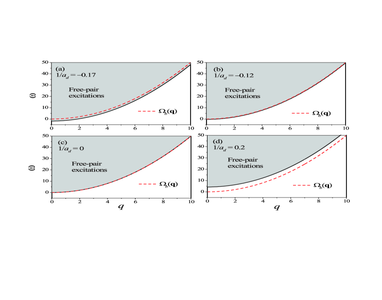
Figure 4: (color online) Excitation region of a gas of interacting fermions in $\left(q,\omega\right)$-space (the case of the d-wave scattering) at $T=T_{c}$ for $k_{0}=10$, $k_{1}=10$, and $\cos\theta=1/2$. The shaded area shows the continuum of the two-particle excitations. The black curve denotes the lower-frequency bound of the damping area. The dashed red curve shows the points given by $\omega=\Omega_{b}\left(\mathbf{q}\right)$, where $\Omega_{b}\left(\mathbf{q}\right)=\omega_{b}\left(\mathbf{q}\right)-2\mu$ with the energy $\omega_{b}\left(\mathbf{q}\right)$ of the two-body bound state.

In Fig. 4, we have plotted the excitation region of the fermion gas in $\left(q,\omega\right)$-space for the d-wave scattering at different values of the inverse scattering length $1/a_{d}$ and at $T=T_{c}$. The solid black curve denotes the the lower bound $\omega_{0}\left(q\right)=q^{2}/2-2\mu$ for the continuum of free two-particle excitations, which is determined by the inequality $\omega>\omega_{0}\left(q\right)$. The dashed red curve corresponds to the solution of the equation $\omega=\Omega_{b}\left(\mathbf{q}\right)$, where $\Omega_{b}\left(\mathbf{q}\right)$ is the pole of the structure factor $S\left(\mathbf{q},\omega\right)$. In the case when $\Omega_{b}\left(\mathbf{q}\right)<\omega_{0}\left(q\right)$, i. e., when the pole $\Omega_{b}\left(\mathbf{q}\right)$ lies outside the continuum of two-particle excitations, $\Omega_{b}\left(\mathbf{q}\right)$ is given by $\Omega_{b}\left(\mathbf{q}\right)=\omega_{b}\left(\mathbf{q}\right)-2\mu,$ where $\omega_{b}\left(\mathbf{q}\right)$ is the energy of the two-body bound state demelo1993 . In the strong-coupling limit, the energy of the two-body bound state tends to $\omega_{b}\left(\mathbf{q}\right)=-E_{b}+q^{2}/2$, where $E_{b}$ is the pair binding energy, which in this limit and at $T=T_{c}$ tends to $\left(-2\mu\right)$. For a sufficiently weak coupling, the pole $\Omega_{b}\left(\mathbf{q}\right)$ lies within the continuum, and therefore the two-body bound state is damped.

In the case of $d$-wave scattering, for all considered values of $q$, the two-body bound states are damped at $1/a_{d}<0$ [Fig. 4 (a, b)] and non-damped at $1/a_{d}\gtrapprox 0$ [Fig. 4 (d)]. For $1/a_{d}=0$ [Fig. 4 (c)], $\omega_{0}\left(q\right)$ and $\Omega_{b}\left(q\right)$ practically coincide. This allows to interpret, in the case of $d$-wave scattering, the value $1/a_{d}=0$ as the boundary between the regimes of the BCS-pairing (for $1/a_{d}<0$) and the BEC-pairing (for $1/a_{d}\gtrapprox 0$).

The 3D plots in Fig. 5 represent the structure factors for the s-wave and d-wave pairing at weak-coupling. Because the scattering potential for the $d$-wave scattering is angle-dependent, the structure factor $S\left(\mathbf{q},\omega\right)$ depends on three variables: $S\left(\mathbf{q},\omega\right)=S\left(q,\cos\theta,\omega\right)$. Here, we discuss the results for $S\left(q,\omega\right)$ averaged over the directions,

$$S\left(q,\omega\right)\equiv\frac{1}{2}\int_{0}^{\pi}S\left(\mathbf{q},\omega\right)\sin\theta d\theta.$$ (48)

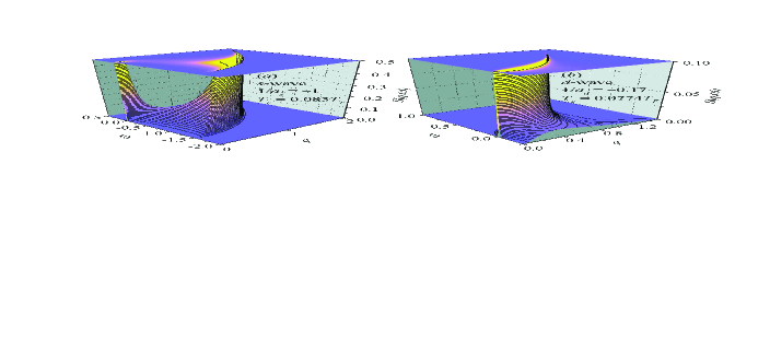
Figure 5: (color online) 3D plot of the structure factor $S\left(q,\omega\right)$ for the $s$-wave scattering (a) and for the $d$-wave scattering (b) at $T=T_{c}$ in the weak-coupling regime. The critical temperatures are given in units of the Fermi temperature $T_{F}\equiv\hbar^{2}k_{F}^{2}/\left(2mk_{B}\right)$. At the top, there are the contour density plots for $S\left(q,\omega\right)$.

In Fig. 5 (a), the structure factor for the case of $s$-wave pairing is shown for $1/a_{s}=-1$, which lies on the BCS side of the resonance. In the BCS regime, the poles corresponding to the two-body pair excitations are damped since they lie in the continuum area. The spectral weight of those poles in the overall structure factor is significant only at small wave vectors. This results in a peak around $q=0$ in Fig. 5 (a). Furthermore, there is a distinctive extremum of the structure factor at the boundary of the continuum of two-particle excitations. In Fig. 5 (b) we switch from $s$-wave to $d$-wave pairing, but remain within on BCS side of the resonance: this panel shows the structure factor for the $d$-wave pairing is for $1/a_{d}=-0.17$. This value of the $d$-wave scattering length is close to the lowest value of the inverse scattering length at which pairing can occur. Also in the $d$-wave BCS regime, the two-body bound states are damped and therefore the peak corresponding to the two-body bound excitations has a finite width. However, the width of that peak in the case of the $d$-wave scattering is relatively low. From this we can see that in the case of the $d$-wave scattering, the two-body bound state plays a significant role even in the weak-coupling regime. For the $d$-wave scattering, as distinct from the $s$-wave scattering, the BCS pairing mechanism can be realized only in a narrow range of the inverse scattering length close to the lowest value of $1/a_{d}$ from those, for which pairing can occur.

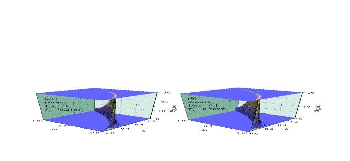
Figure 6: (color online) 3D plot of the structure factor $S\left(q,\omega\right)$ for the $s$-wave scattering (a) and for the $d$-wave scattering (b) at $T=T_{c}$ in the strong-coupling regime.

Fig. 6 describes the strong-coupling case (on the BEC side of the resonance) where there is a non-damped isolated pole in the structure factor. Therefore, the structure factor in the strong-coupling regime contains a $\delta$-like peak, which lies outside the continuum of free-pair excitations. In order to visualize those $\delta$-like peaks, we use a finite damping parameter $\gamma=0.01$. In the strong-coupling regime, the regular part of $S\left(\mathbf{q},\omega\right)$ is negligibly small with respect to the main contribution due to the aforesaid isolated pole, which describes the BEC pairing.

VI Discussion and conclusions

VI.1 The unitarity limit

A first point to discuss, is the predicament of mean-field theory in the unitarity limit, $1/a\rightarrow 0$. It is crucial that fluctuations are taken into account, as we have done in the previous section. Higher-order fluctuation contributions can be taken into account, and many different approaches were developed for the balanced $s$-wave Fermi superfluid. These approaches differ in the types of higher-order processes they take into account. Strinati and co-workers strinati work diagrammatically to improve on the results obtained by Nozières and Schmitt-Rink for $T=T_{c}$. Levin and co-workers levin construct a finite temperature theory similar to that of Strinati and co-workers but include different diagrams in the summation. Alternatively, quantum Monte Carlo simulations MC can be used to obtain results on the crossover physics the balanced $s$-wave Fermi superfluid and put the crossover theories to the test . At the unitarity limit the existing theories do not succeed to find the free energy of the system with more than 10% accuracy with respect to the Monte Carlo results. As such, we expect the current theory to have a similar level of accuracy in the unitarity limit for the $d$-wave system.

The problem that lies at the root of the difficulty to make a theory for unitarity is that one needs to take into account not only the fluctuations of the order parameter but also the normal-state interactions correctly. The diagrammatic approaches strinati ; levin are based on a zeroth-order decoupling that emphasizes pair formation rather than normal-state interactions. Put in the language of functional integrationRanderia2007 , we have made a particular choice for the Hubbard-Stratonovic decoupling: we took $\bar{\psi}\bar{\psi}$ and $\psi\psi$ types of products of Grassmann variables. This emphasizes pairing, but when the pairing goes to zero at the saddle-point, the resulting normal state has no interactions, and fluctuation corrections are needed to remedy this. We could have made the choice to group $\bar{\psi}\psi$ and $\bar{\psi}\psi$ and apply the Hubbard-Stratonovic scheme to decouple the four-product in these densities rather than in the pairs. The resulting saddle-point approximation would yield the random phase approximation (RPA) results for the interacting normal state; but it would lack pairing. The inability to include –on the level of a saddle-point approximation– both pairing and RPA normal-state interactions through the introduction of two collective fields is discussed by Kleinert kleinert1 , who proposes variational perturbation theory as a solutionkleinert2 . The fluctuation expansion used in the current work goes beyond that of Ref.Randeria2007 , in that we take not only the particle-pair $\bar{\psi}\bar{\psi}$ and hole-pair $\psi\psi$ excitations, but also particle-hole terms $\bar{\psi}\psi$ are present. These contributions appear in terms that do not vanish as the saddle point goes to zero, $\Delta\rightarrow 0$, so that the normal state in the present treatment is the interacting Fermi gas rather than the ideal Fermi gas. As such, the present treatment will be better suited in the unitary limit.

VI.2 Routes for experimental observation

Magnetically tuning the population imbalance in a Fermi superfluid is out of reach at present in high-temperature superconductors. In cold atomic gases it has been successfully demonstrated and applied to reach the superfluid regime. The currently realized atomic Fermi superfluids have $s$-wave symmetry of the order parameter. The $d$-wave coupling strength generally is too small to dominate the $s$-wave scattering at low temperature. This can be overcome using a Feshbach resonance in the $d$-wave scattering channel. $d$-wave Feshbach resonances have been observed, for example, in various isotopes of rubidiumdwavefesh . However, to reach the unitary limit for the $d$-wave scattering one needs a better control over the magnetic field than in the $s$-wave case, since the interaction parameter $\lambda,$ expression (26), scales as $a_{d}^{-5}$ as compared to $a_{s}^{-1}$. The current results suggest a different route towards $d$-wave superfluidity: imbalancing the gas. The dominant $s$-wave pairing is easily suppressed on the BCS side of the resonance by adding imbalance, whereas $d$-wave superfluidity is less sensitive to imbalance. Both the use of a $d$-wave Feshbach resonance to obtain a large enough $d$-wave coupling strength, and of imbalance to suppress $s$-wave pairing, will be needed to realize $d$-wave superfluidity in the atomic gases.

In an inhomogneous trapping potential, phase separation can occur in real space. For $s$-wave superfluidity, this leads to a balanced superfluid at the center of the trap, surrounded by a halo of imbalanced (or fully polarized) normal gas pilatiPRL100 . In effect, the excess spin component has been expelled from the balanced $s$-wave superfluid. The additional energy cost of placing the excess atoms fhigher up the trapping potential is compensated by the energy gained by allowing the balanced superfluid state to form. In the $d$-wave superfluid, this energy balance is different. Increasing imbalance in the BCS side does not strongly reduce the free energy of the superfluid. As can be seen from Fig. 2, the $d$-wave order parameter is not strongly affected. Therefore, expelling the excess atoms to the edge of the trap raises the total energy and we do not expect real-space phase separation. The situation is different on the BEC side: here, the free energy of the $d$-wave superfluid is reduced by imbalance, and it becomes energetically favourable to expell excess atoms.

VI.3 Exotic pairing scenarios

Note that the action for the fluctuations depends (through $\mathcal{M}_{11}$ and $\mathcal{M}_{21}$) on the choice of saddle point $\Delta$. This means that the spectrum of excitations (obtained from the diagonalized fluctuation action) also depends on the choice of the saddle point. Excitations for a vortex condensate may be different from excitations on top of a ground-state condensate. At nonzero temperature those excitations will be populated through Bose statistics. But the physics is more complex than just Bose populating excitations: the excitation spectrum itself (the dispersion and lifetime of those excitations) is temperature dependent: new single-particle and collective modes appear and shift as a function of temperature. At zero temperature the only single-particle excitations are $E_{\mathbf{k}}$, the energy spectrum for breaking a Cooper pair, but at finite temperature, we also have the excitations of the thermal gas. These consist in taking the atoms of a broken Cooper pair, and giving those atoms an extra kick: $E_{\mathbf{k+q}}-E_{\mathbf{k}}$. Besides those single-particle excitations, we will have collective excitations whenever $\mathcal{M}_{11}\mathcal{M}_{22}\mathcal{-M}_{21}\mathcal{M}_{12}=0$.

In the case of an imbalanced Fermi gas, an alternative choice for the saddle point is $\Delta e^{i\mathbf{kr}}$ where k represent a shortest wave vector connecting the Fermi surface of the minority component to that of the majority component. The resulting equations describe the Fulde-Ferrell-Larkin-Ovchinnikov state FFLO ; yoshida . However, this state has not yet been reported experimentally, so we have restricted the present analysis to the usual pairing scenario.

VI.4 Conclusions

We have investigated the imbalanced d-wave Fermi gas, both at zero and at nonzero temperatures, and as a function of the $d$-wave interaction strength. We find that in the BCS regime, the $d$-wave pairing is more robust to the presence of population imbalance than the $s$-wave case. For a range of interaction strengths, we find that the $s$-wave superfluidity is suppressed whereas the $d$-wave superfluidity is not. This is shown to be related to the possibility of creating a polarized gas of excitations in the nodes of the gap. Rather than phase separation in real space, phase separation can occur in reciprocal space. An additional difference with the $s$-wave BCS case, is that a critical attraction strength is needed in the $d$-wave case before pairing can occur (in $s$-wave pairing occurs for all attractive interaction strengths). In the BEC regime, the symmetry of the pairing interaction plays a less important role: as the molecule gets more tightly bound, the details of its internal wave function matter less, and we retrieve known results for the $s$-wave system in the same BEC limitOhashiPRA67 ; strinati ; levin . We then investigate how our results are affected by Gaussian fluctuations, important both to describe the nonzero-temperature thermodynamics. Both the critical temperature and the effect of temperature on the spectral density of the excitations are calculated. Our investigation of the structure factor reveals that for the $d$-wave scattering, the damping of the pole for $S\left(\mathbf{q},\omega\right)$ is very small even in the BCS regime, in contrast to that for the $s$-wave scattering. The critical temperature in the BCS regime reflects the pair binding energy. This implies that the critical temperature for the $d$-wave superfluid in the BCS regime will also be more robust against population imbalance.

Appendix A Matsubara summation for the density

Let us consider the contour integral on the contour $C$ shown in Fig. 7:

$$I\equiv\frac{1}{2\pi i}\oint\nolimits_{C}\frac{f\left(z\right)}{e^{\beta z}-1}dz,$$ (49)

where the points $z=i\Omega_{n}$ with $\left|n\right|>n_{0}$ lie inside the contour, and the other points $z=i\Omega_{n}$ are outside the contour. The function $f\left(z\right)$ possesses the following properties: (i) it is analytic in the entire complex $z$-plane except, possibly, the branching line on the real axis, (ii) $f\left(z\right)$ decreases at $\operatorname{Re}z\rightarrow-\infty$ faster than $z^{-1}$, so that the integral $\int_{-\infty}^{0}f\left(\omega\pm i\gamma\right)d\omega$, where $\omega$ and $\gamma$ are real, converges. The functions $J\left(\mathbf{q},z\right)$ and $K\left(\mathbf{q},z\right)$ determined, respectively, by Eqs. (37) and (38), satisfy these conditions. The fraction $\frac{1}{e^{\beta z}-1}$ has the poles at $z=i\Omega_{n}$, $n=0,\pm 1,\pm 2,\ldots$. The residues of $\frac{1}{e^{\beta z}-1}$ in the points $z=i\Omega_{n}$ are equal to $\frac{1}{\beta}$.

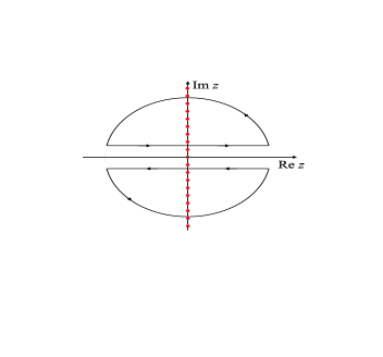
Figure 7: (color online) Integration contour in the complex $z$-plane. The full dots indicate the poles $z=i\Omega_{n}$, $n=0,\pm 1,\pm 2,\ldots$.

On the one hand, the integral (49) is equal to the sum of the residues of the function $\frac{f\left(z\right)}{e^{\beta z}-1}$ in the points $z=i\Omega_{n}$ inside the contour $C$:

$$I=\frac{1}{\beta}\sum_{\left|n\right|>n_{0}}f\left(i\Omega_{n}\right),$$ (50)

On the other hand, the integral $I$ is

$$I=\frac{1}{2\pi i}\int_{-\infty}^{\infty}\frac{f\left(\omega+i\gamma\right)}{e^{\beta\left(\omega+i\gamma\right)}-1}d\omega-\frac{1}{2\pi i}\int_{-\infty}^{\infty}\frac{f\left(\omega-i\gamma\right)}{e^{\beta\left(\omega-i\gamma\right)}-1}d\omega,$$ (51)

where the parameter $\gamma$ satisfies the inequality

$$\Omega_{n_{0}}<\gamma<\Omega_{n_{0}+1}.$$ (52)

It follows from the equivalence of (50) and (51) that

$$\sum_{n}f\left(i\Omega_{n}\right)=\frac{\beta}{\pi}\int_{-\infty}^{\infty}\operatorname{Im}\left[\frac{f\left(\omega+i\gamma\right)}{e^{\beta\left(\omega+i\gamma\right)}-1}\right]d\omega+\sum_{n=-n_{0}}^{n_{0}}f\left(i\Omega_{n}\right).$$ (53)

According to the theorem (53), the fluctuation contributions to the density and to the population imbalance can be represented as

$$n_{fl} =-\int\frac{d\mathbf{q}}{\left(2\pi\right)^{3}}\left(\frac{1}{\pi}\int_{-\infty}^{\infty}\operatorname{Im}\left[\frac{J\left(\mathbf{q},\omega+i\gamma\right)}{e^{\beta\left(\omega+i\gamma\right)}-1}\right]d\omega+\frac{1}{\beta}\sum_{n=-n_{0}}^{n_{0}}J\left(\mathbf{q},i\Omega_{n}\right)\right),$$ (54)

$$\delta n_{fl} =-\int\frac{d\mathbf{q}}{\left(2\pi\right)^{3}}\left(\frac{1}{\pi}\int_{-\infty}^{\infty}\operatorname{Im}\left[\frac{K\left(\mathbf{q},\omega+i\gamma\right)}{e^{\beta\left(\omega+i\gamma\right)}-1}\right]d\omega+\frac{1}{\beta}\sum_{n=-n_{0}}^{n_{0}}K\left(\mathbf{q},i\Omega_{n}\right)\right).$$ (55)

As follows from the above analytical transformations of the integrals in the complex $z$-plane, the sum (53) does not depend on the choice of the number $n_{0}$ and (for a given $n_{0}$) on the value of $\gamma$ within the range given by (52).

References

- (1) also at Lyman Laboratory of Physics, Harvard University, Cambridge MA 02138, USA.
- (2) C.A. Regal, M. Greiner, and D. Jin, Phys. Rev. Lett. 92, 040403 (2004); M. W. Zwierlein et al., Phys. Rev. Lett. 92, 120403 (2004); T. Bourdel et al., Phys. Rev. Lett. 93, 050401 (2004); G. B. Partridge et al., Phys. Rev. Lett. 95, 020404 (2005).
- (3) M. Greiner, C.A. Regal and D. Jin, Nature 426, 537 (2003); S. Jochim et al., Science 302, 2101 (2003), M.W. Zwierlein et al., Phys. Rev. Lett. 91, 120403 (2003).
- (4) M.W. Zwierlein, A. Schirotzek, C.H. Schunck, and W. Ketterle, Science 311, 492-496 (2006).
- (5) G.B. Partridge, W. Li, R.I. Kamar, Y.-A. Liao, and R. G. Hulet, Science 311, 503-505 (2006); G. B. Partridge, Wenhui Li, Y. A. Liao, R. G. Hulet, M. Haque and H. T. C. Stoof, Phys. Rev. Lett. 97, 190407 (2006).
- (6) A. Sedrakian et al., Phys. Rev. A 72, 013613 (2005); C.-H. Pao and S.-T. Wu, S.-K. Yip, Phys. Rev. B 73, 132506 (2006); D. E. Sheehy and L. Radzihovsky, Phys. Rev. Lett. 96, 060401 (2006); J. Dukelsky et al., ibid. 96, 180404 (2006); P. Pieri and G. C. Strinati, ibid. 96, 150404 (2006); J. Kinnunen, L. M. Jensen, and P. Torma, ibid. 96, 110403 (2006); F. Chevy, ibid. 96, 130401 (2006); K. Machida, T. Mizushima, and M. Ichioka, ibid. 97, 120407 (2006); M. Haque and H. T. C. Stoof, Phys. Rev. A 74, 011602 (2006).
- (7) A.M. Clogston, Phys. Rev. Lett. 9, 266 (1962).
- (8) T.N. De Silva and E.J. Mueller, Phys. Rev. A 73, 051602 (2006).
- (9) P. Fulde and R. A. Ferrell, Phys. Rev. 135, A550 (1964); A. I. Larkin and Y. N. Ovchinnikov, Sov. Phys. JETP 20, 762 (1965).
- (10) G. Sarma, J. Phys. Chem. Solids 24, 1029 (1963).
- (11) M. Randeria, in Bose Einstein Condensation, edited by A. Griffin, D. Snoke, and S. Stringari (Cambridge Univ. Press, Cambridge, 1995), pp. 355–92; Q. Chen, J. Stajic, and K. Levin, Low. Temp. Phys. 32, 406 (2006) [Fiz. Nizk. Temp. 32, 538 (2006)].
- (12) M. C. Boyer, W. D. Wise, K. Chatterjee, M. Yi, T. Kondo, T. Takeuchi, H. Ikuta, and E. W. Hudson, Nature Physics 3, 802 (01 Nov 2007).
- (13) G. V. M. Williams, J. L. Tallon, E. M. Haines, R. Michalak, and R. Dupree, Phys. Rev. Lett. 78, 721 (1997).
- (14) The mounting evidence for the preformed pair scenario in high-Tc superconductors is described in A. S. Alexandrov, in Theory of Superconductivity: From Weak to Strong Coupling (IoP Publishing, Bristol-Philadelphia, 2003), and references therein.
- (15) A. S. Alexandrov and P. E. Kornilovitch, J. Phys. Condens.Matter 14, 5337 (2002); A. S. Alexandrov and A. F. Andreev, Europhys. Lett. 54, 373 (2001).
- (16) M. Wouters, J. Tempere, J.T. Devreese, Phys. Rev. A 70, 013616 (2004); J. Tempere, M. Wouters and J.T. Devreese, Phys. Rev. B 75, 184526 (2007).
- (17) J. Tempere, M. Wouters, J.T. Devreese, Phys. Rev. A 71, 033631 (2005); J. Tempere, J.T. Devreese, to appear in Physica C.
- (18) C. A. R. Sá de Melo, M. Randeria, and J. R. Engelbrecht, Phys. Rev. Lett. 71, 3202 (1993)
- (19) P. Nozières and S. Schmitt-Rink, J. Low Temp. Phys. 59, 195 (1985).
- (20) E. Taylor, A. Griffin, N. Fukushima, and Y. Ohashi, Phys. Rev. A 74, 063626 (2006).
- (21) J. R. Engelbrecht, M. Randeria, and C. A. R. Sá de Melo, Phys. Rev. B55, 15153 (1997).
- (22) R. B. Diener, R. Sensarma, and M. Randeria, arXiv:0709.2653v1 (2007).
- (23) N. Fukushima, Y. Ohashi, E. Taylor, and A. Griffin, Phys. Rev. A 75, 033609 (2007).
- (24) R. D. Duncan and C. A. R. Sá de Melo, Phys. Rev. B 62, 9675 (2000).
- (25) M. Iskin, C.A.R. Sá de Melo, Phys. Rev. Lett. 96, 040402 (2006).
- (26) Z. Izdiaszek & T. Calarco, Phys. Rev. Lett. 96, 013206 (2006).
- (27) P. Nozières and S. Schmitt-Rink, J. Low Temp. Phys. 59, 195 (1985).
- (28) C. A. Regal, C. Ticknor, J. L. Bohn, and D. S. Jin, Phys. Rev. Lett. 90, 053201 (2003).
- (29) Y. Ohashi and A. Griffin, Phys. Rev. A 67, 063612 (2003).
- (30) A. Perali, P. Pieri, L. Pisani, G.C. Strinati, Phys. Rev. Lett. 92, 220404 (2004).
- (31) Q. Chen, Y. He, C.C. Chien, K. Levin, Phys. Rev. B 75, 014521 (2007).
- (32) S. Y. Chang, V. R. Pandharipande, J. Carlson, and K. E. Schmidt, Phys. Rev. A 70, 043602 (2004); G. E. Astrakharchik, J. Boronat, J. Casulleras, and S. Giorgini, Phys. Rev. Lett. 93, 200404 (2004).
- (33) H. Kleinert, Fortschr. Physik 26, 55 (1978).
- (34) H. Kleinert, Annals of Physics 266, 135 (1998).
- (35) S. Pilati and S. Giorgini, Phys. Rev. Lett. 100, 030401 (2008).
- (36) H. M. J. M. Boesten et al., Phys. Rev. A 55, 636 (1997); J. P. Burke and J. L. Bohn, Phys. Rev. A 59, 1303 (1999).
- (37) N. Yoshida and S.-K. Yip, Phys. Rev. A 75, 063601 (2007)