Hopf Bifurcations in a
Watt Governor with a Spring

Jorge Sotomayor

Instituto de Matemática e Estatística, Universidade de São Paulo
Rua do Matão 1010, Cidade Universitária
CEP 05.508-090, São Paulo, SP, Brazil
e–mail:sotp@ime.usp.br

Luis Fernando Mello

Instituto de Ciências Exatas, Universidade Federal de Itajubá
Avenida BPS 1303, Pinheirinho, CEP 37.500-903, Itajubá, MG, Brazil
e–mail:lfmelo@unifei.edu.br

Denis de Carvalho Braga

Instituto de Sistemas Elétricos e Energia, Universidade Federal de Itajubá
Avenida BPS 1303, Pinheirinho, CEP 37.500-903, Itajubá, MG, Brazil
e–mail:braga@unifei.edu.br

Abstract

This paper pursues the study carried out by the authors in Stability and Hopf bifurcation in a hexagonal governor system [13], focusing on the codimension one Hopf bifurcations in the hexagonal Watt governor differential system. Here are studied the codimension two, three and four Hopf bifurcations and the pertinent Lyapunov stability coefficients and bifurcation diagrams, illustrating the number, types and positions of bifurcating small amplitude periodic orbits, are determined. As a consequence it is found an open region in the parameter space where two attracting periodic orbits coexist with an attracting equilibrium point.

Key-words: Centrifugal governor, Watt governor, Hopf bifurcation, stability, periodic orbits.

MSC: 70K50, 70K20.

1 Introduction

The centrifugal governor is a device that automatically controls the speed of an engine. The most important one is due to James Watt –Watt governor– and it can be taken as the starting point for automatic control theory. Centrifugal governor design received several important modifications as well as other types of governors were also developed. From MacFarlane [8], p. 251, we quote:

“Several important advances in automatic control technology were made in the latter half of the 19th century. A key modification to the flyball governor was the introduction of a simple means of setting the desired running speed of the engine being controlled by balancing the centrifugal force of the flyballs against a spring, and using the preset spring tension to set the running speed of the engine”.

In this paper the system coupling the Watt governor with a spring (resp. Watt governor) and the steam engine will be called simply the Watt Governor System with Spring (WGSS) (resp. Watt Governor System (WGS)). The stability analysis of the stationary states and small amplitude oscillations of this system will be pursued here.

The first mathematical analysis of the stability conditions in the WGS was due to Maxwell [9] and, in a user friendly style likely to be better understood by engineers, by Vyshnegradskii [15]. A simplified version of the WGS local stability based on the work of Vyshnegradskii is presented by Pontryagin [10].

From the mathematical point of view, the oscillatory, small amplitude, behavior in the WGS can be associated to a periodic orbit that appears from a Hopf bifurcation. This was established by Hassard et al. in [5], Al-Humadi and Kazarinoff in [1] and by the authors in [11, 12]. Another procedure, based in the method of harmonic balance, has been suggested by Denny [3] to detect large amplitude oscillations.

In [11] we characterized the surface of Hopf bifurcations in a WGS, which is more general than that presented by Pontryagin [10], Al-Humadi and Kazarinoff [1] and Denny [3].

In [12] restricting ourselves to Pontryagin’s system of differential equations for the WGS, we carried out a deeper investigation of the stability of the equilibrium along the critical Hopf bifurcations up to codimension 3, happening at a unique point at which the bifurcation diagram was established. A conclusion derived from the diagram implied the existence of parameters where the WGS has an attracting periodic orbit coexisting with an attracting equilibrium.

In [13] we characterized the hypersurface of Hopf bifurcations in a WGSS. See Theorem 4.1 and Fig. 2 for a review of the critical surface where the first Lyapunov coefficient vanishes.

In the present paper we go deeper investigating the stability of the equilibrium along the above mentioned critical surface. To this end the second Lyapunov coefficient is calculated and it is established that it vanishes along two curves. The third Lyapunov coefficient is calculated on these curves and it is established that it vanishes at a unique point. The fourth Lyapunov coefficient is calculated at this point and found to be negative. See Theorem 4.2. The pertinent bifurcation diagrams are established. See Fig. 6 and 7. A conclusion derived from these diagrams, concerning the region —a solid “tongue”— in the space of parameters where two attracting periodic orbits coexist with an attracting equilibrium, is specifically commented in Section 5.

The extensive calculations involved in Theorem 4.2 have been corroborated with the software MATHEMATICA 5 [17] and the main steps have been posted in the site [16].

This paper is organized as follows. In Section 2 we introduce the differential equations that model the WGSS. The stability of the equilibrium point of this model is analyzed and a general version of the stability condition is obtained and presented in the terminology of Vyshnegradskii. The Hopf bifurcations in the WGSS differential equations are studied in Sections 3 and 4. Expressions for the second, third and fourth Lyapunov coefficients, which fully clarify their sign, are obtained, pushing forward the method found in the works of Kuznetsov [6, 7]. With this data, the bifurcation diagrams are established. Concluding comments, synthesizing and interpreting the results achieved here, are presented in Section 5.

2 The Watt governor system with spring

2.1 WGSS differential equations

The WGSS studied in this paper is shown in Fig. 1. There, $\varphi\in\left(0,\frac{\pi}{2}\right)$ is the angle of deviation of the arms of the governor from its vertical axis $S_{1}$, $\Omega\in[0,\infty)$ is the angular velocity of the rotation of the engine flywheel $D$, $\theta$ is the angular velocity of the rotation of $S_{1}$, $l$ is the length of the arms, $m$ is the mass of each ball, $H$ is a sleeve which supports the arms and slides along $S_{1}$, $T$ is a set of transmission gears and $V$ is the valve that determines the supply of steam to the engine.

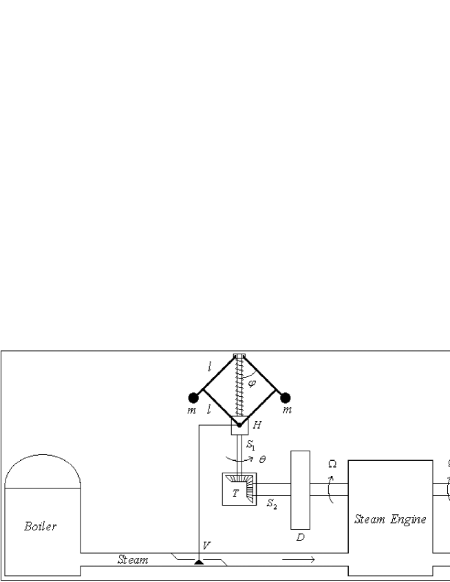
Figure 1: Watt centrifugal governor with a spring – steam engine system.

The WGSS differential equations can be found as follows. For simplicity, we neglect the mass of the sleeve and the arms. There are four forces acting on the balls at all times. They are the tangential component of the gravity

$$-mg\sin\varphi,$$

where $g$ is the standard acceleration of gravity; the tangential component of the centrifugal force

$$m\;l\;\sin\varphi\;\theta^{2}\cos\varphi;$$

the tangential component of the restoring force due to the spring

$$-2kl(1-\cos\varphi)\sin\varphi,$$

$2l$ is the natural length of the spring and $k\geq 0$ is the spring constant; and the force of friction

$$-bl\dot{\varphi},$$

$b>0$ is the friction coefficient.

From the Newton’s Second Law of Motion, and using the transmission function $\theta=c\>\Omega$, where $c>0$, one has

$$\ddot{\varphi}=\left(\frac{2k}{m}+c^{2}\Omega^{2}\right)\sin\varphi\cos\varphi-\frac{2kl+mg}{ml}\>\sin\varphi-\frac{b}{m}\>\dot{\varphi}.$$ (1)

The torque acting upon the flywheel $D$ is

$$I\>\dot{\Omega}=\mu\>\cos\varphi-F,$$ (2)

where $I$ is the moment of inertia of the flywheel, $F$ is an equivalent torque of the load and $\mu>0$ is a proportionality constant. See [10], p. 217, for more details.

From Eq. (1) and (2) the differential equations of our model are given by

$$\frac{d\;\varphi}{d\tau} = \psi$$

$$\frac{d\;\psi}{d\tau} = \left(\frac{2k}{m}+c^{2}\Omega^{2}\right)\sin\varphi\cos\varphi-\frac{2kl+mg}{ml}\;\sin\varphi-\frac{b}{m}\;\psi$$ (3)

$$\frac{d\;\Omega}{d\tau} = \frac{1}{I}\;\left(\mu\cos\varphi-F\right)$$

where $\tau$ is the time.

The standard Watt governor differential equations in Pontryagin [10], p. 217,

$$\frac{d\;\varphi}{d\tau} = \psi$$

$$\frac{d\;\psi}{d\tau} = c^{2}\;\Omega^{2}\;\sin\varphi\;\cos\varphi-\frac{g}{l}\;\sin\varphi-\frac{b}{m}\;\psi$$ (4)

$$\frac{d\;\Omega}{d\tau} = \frac{1}{I}\;\left(\mu\cos\varphi-F\right)$$

are obtained from (2.1) by taking $k=0$.

Defining the following changes in the coordinates, parameters and time

$$x=\varphi,\>y=\left(\frac{ml}{2kl+mg}\right)^{1/2}\psi,\>z=c\left(\frac{ml}{2kl+mg}\right)^{1/2}\Omega,$$

$$t=\left(\frac{2kl+mg}{ml}\right)^{1/2}\tau,\>\kappa=\frac{2kl}{2kl+mg},$$

$$\varepsilon=\frac{b}{m}\left(\frac{ml}{2kl+mg}\right)^{1/2},\>\alpha=\frac{c\mu}{I}\left(\frac{ml}{2kl+mg}\right),\>\beta=\frac{F}{\mu},$$

where $0\leq\kappa<1$, $\varepsilon>0$, $\alpha>0$ and $0<\beta<1$, the differential equations (2.1) can be written as

$$x^{\prime}=\frac{dx}{dt} = y$$

$$y^{\prime}=\frac{dy}{dt} = (z^{2}+\kappa)\;\sin x\;\cos x-\sin x-\varepsilon\;y$$ (5)

$$z^{\prime}=\frac{dz}{dt} = \alpha\;(\cos x-\beta)$$

or equivalently by

$${\bf x}^{\prime}=f({\bf x},{\bf\zeta}),$$ (6)

where

$$f({\bf x},{\bf\zeta})=\left(y,(z^{2}+\kappa)\;\sin x\;\cos x-\sin x-\varepsilon\;y,\alpha\;\left(\cos x-\beta\right)\right),$$

$${\bf x}=(x,y,z)\in\left(0,\frac{\pi}{2}\right)\times\mathbb{R}\times[0,\infty)$$

and

$${\bf\zeta}=(\beta,\alpha,\varepsilon,\kappa)\in\left(0,1\right)\times\left(0,\infty\right)\times\left(0,\infty\right)\times\left[0,1\right).$$

2.2 Stability analysis of the equilibrium point

The WGSS differential equations (2.1) have only one admissible equilibrium point

$$P_{0}=(x_{0},y_{0},z_{0})=\left(\arccos\beta,0,\left(\frac{1}{\beta}-\kappa\right)^{1/2}\right).$$ (7)

The Jacobian matrix of $f$ at $P_{0}$ has the form

$$Df\left(P_{0}\right)=\left(\begin{array}[]{ccc}0&1&0\\ \\ -\omega_{0}^{2}&-\varepsilon&\xi\\ \\ -\alpha(1-\beta^{2})^{1/2}&0&0\end{array}\right),$$ (8)

where

$$\omega_{0}=\sqrt{\frac{1-\beta^{2}}{\beta}}$$ (9)

and

$$\xi=2\beta^{1/2}(1-\beta^{2})^{3/4}(1-\kappa\beta)^{1/2}.$$

For the sake of completeness we state the following lemma whose proof can be found in [10], p. 58.

Lemma 2.1

The polynomial $L(\lambda)=p_{0}\lambda^{3}+p_{1}\lambda^{2}+p_{2}\lambda+p_{3}$, $p_{0}>0$, with real coefficients has all roots with negative real parts if and only if the numbers $p_{1},p_{2},p_{3}$ are positive and the inequality $p_{1}p_{2}>p_{0}p_{3}$ is satisfied.

Theorem 2.2

If

$$\varepsilon>\varepsilon_{c}=2\;\alpha\;\beta^{3/2}(1-\kappa\beta)^{1/2},$$ (10)

then the WGSS differential equations (2.1) have an asymptotically stable equilibrium point at $P_{0}$. If

$$0<\varepsilon<\varepsilon_{c}$$

then $P_{0}$ is unstable.

Proof. The characteristic polynomial of $Df\left(P_{0}\right)$ is given by $p(\lambda)$, where

$$-p(\lambda)=\lambda^{3}+p_{1}\>\lambda^{2}+p_{2}\>\lambda+p_{3},$$

$$p_{1}=\varepsilon,\>\>p_{2}=\frac{1-\beta^{2}}{\beta},\>\>p_{3}=\frac{2\alpha\beta^{3/2}(1-\beta^{2})(1-\kappa\beta)^{1/2}}{\beta}.$$

The coefficients of $-p(\lambda)$ are positive. Thus a necessary and sufficient condition for the asymptotic stability of the equilibrium point $P_{0}$, as provided by the condition for one real negative root and a pair of complex conjugate roots with negative real part, is given by (10), according to Lemma 2.1.

$\blacksquare$

In terms of the WGSS physical parameters, condition (10) is equivalent to

$$\frac{b\>I}{m}\>\eta>1,$$ (11)

where

$$\eta=\left|\frac{d\Omega_{0}}{dF}\right|=\frac{1}{2\beta^{3/2}(1-\kappa\beta)^{1/2}}$$ (12)

is the non-uniformity of the performance of the engine which quantifies the change in the engine speed with respect to the load (see [10], p. 219, for more details). Eq. (12) can be easily written in terms of the original parameters.

The rules formulated by Vyshnegradskii to enhance the stability follow directly from (11). In particular, the interpretation of (11) is that a sufficient amount of damping $b$ must be present relative to the other physical parameters for the system to be stable at the desired operating speed. The condition (11) is equivalent to the original condition given by Vyshnegradskii for the WGS (see [10], p. 219).

In section 4 we study the stability of $P_{0}$ under the condition

$$\varepsilon=\varepsilon_{c},$$ (13)

that is, on the hypersurface —the Hopf hypersurface— complementary to the range of validity of Theorem 2.2.

3 Lyapunov coefficients

The beginning of this section is a review of the method found in [6], pp 177-181, and in [7] for the calculation of the first and second Lyapunov coefficients. The calculation of the third Lyapunov coefficient can be found in [12]. The calculation of the fourth Lyapunov coefficient has not been found by the authors in the current literature. The extensive calculations and the long expressions for these coefficients have been corroborated with the software MATHEMATICA 5 [17].

Consider the differential equations

$${\bf x}^{\prime}=f({\bf x},{\bf\mu}),$$ (14)

where ${\bf x}\in\mathbb{R}^{n}$ and ${\bf\mu}\in\mathbb{R}^{m}$ are respectively vectors representing phase variables and control parameters. Assume that $f$ is of class $C^{\infty}$ in $\mathbb{R}^{n}\times\mathbb{R}^{m}$. Suppose (14) has an equilibrium point ${\bf x}={\bf x_{0}}$ at ${\bf\mu}={\bf\mu_{0}}$ and, denoting the variable ${\bf x}-{\bf x_{0}}$ also by ${\bf x}$, write

$$F({\bf x})=f({\bf x},{\bf\mu_{0}})$$ (15)

as

$$F({\bf x})=A{\bf x}+\frac{1}{2}\>B({\bf x},{\bf x})+\frac{1}{6}\>C({\bf x},{\bf x},{\bf x})+\>\frac{1}{24}\>D({\bf x},{\bf x},{\bf x},{\bf x})+\frac{1}{120}\>E({\bf x},{\bf x},{\bf x},{\bf x},{\bf x})+{}$$

$$\frac{1}{720}\>K({\bf x},{\bf x},{\bf x},{\bf x},{\bf x},{\bf x})+\frac{1}{5040}\>L({\bf x},{\bf x},{\bf x},{\bf x},{\bf x},{\bf x},{\bf x})+\frac{1}{40320}\>M({\bf x},{\bf x},{\bf x},{\bf x},{\bf x},{\bf x},{\bf x},{\bf x})$$ (16)

$$+\frac{1}{362880}\>N({\bf x},{\bf x},{\bf x},{\bf x},{\bf x},{\bf x},{\bf x},{\bf x},{\bf x})+O(||{\bf x}||^{10}){},$$

where $A=f_{\bf x}(0,{\bf\mu_{0}})$ and

$$B_{i}({\bf x},{\bf y})=\sum_{j,k=1}^{n}\frac{\partial^{2}F_{i}(\xi)}{\partial\xi_{j}\>\partial\xi_{k}}\bigg{|}_{\xi=0}x_{j}\;y_{k},$$ (17)

$$C_{i}({\bf x},{\bf y},{\bf z})=\sum_{j,k,l=1}^{n}\frac{\partial^{3}F_{i}(\xi)}{\partial\xi_{j}\>\partial\xi_{k}\>\partial\xi_{l}}\bigg{|}_{\xi=0}x_{j}\;y_{k}\>z_{l},$$ (18)

$$D_{i}({\bf x},{\bf y},{\bf z},{\bf u})=\sum_{j,k,l,r=1}^{n}\frac{\partial^{4}F_{i}(\xi)}{\partial\xi_{j}\>\partial\xi_{k}\>\partial\xi_{l}\>\partial\xi_{r}}\bigg{|}_{\xi=0}x_{j}\;y_{k}\>z_{l}\>u_{r},$$ (19)

$$E_{i}({\bf x},{\bf y},{\bf z},{\bf u},{\bf v})=\sum_{j,k,l,r,p=1}^{n}\frac{\partial^{5}F_{i}(\xi)}{\partial\xi_{j}\>\partial\xi_{k}\>\partial\xi_{l}\>\partial\xi_{r}\>\partial\xi_{p}}\bigg{|}_{\xi=0}x_{j}\;y_{k}\>z_{l}\>u_{r}\>v_{p},$$ (20)

$$K_{i}({\bf x},{\bf y},{\bf z},{\bf u},{\bf v},{\bf w})=\sum_{j,\ldots,q=1}^{n}\frac{\partial^{6}F_{i}(\xi)}{\partial\xi_{j}\>\partial\xi_{k}\>\partial\xi_{l}\>\partial\xi_{r}\>\partial\xi_{p}\>\partial\xi_{q}}\bigg{|}_{\xi=0}x_{j}\;y_{k}\>z_{l}\>u_{r}\>v_{p}\>w_{q},$$ (21)

$$L_{i}({\bf x},{\bf y},{\bf z},{\bf u},{\bf v},{\bf w},{\bf t})=\sum_{j,\ldots,h=1}^{n}\frac{\partial^{7}F_{i}(\xi)}{\partial\xi_{j}\partial\xi_{k}\partial\xi_{l}\partial\xi_{r}\partial\xi_{p}\partial\xi_{q}\partial\xi_{h}}\bigg{|}_{\xi=0}x_{j}\;y_{k}\>z_{l}\>u_{r}\>v_{p}\>w_{q}\>t_{h},$$ (22)

$$M_{i}({\bf x},{\bf y},{\bf z},{\bf u},{\bf v},{\bf w},{\bf t},{\bf r})=\sum_{j,\ldots,a=1}^{n}\frac{\partial^{8}F_{i}(\xi)}{\partial\xi_{j}\ldots\partial\xi_{h}\partial\xi_{a}}\bigg{|}_{\xi=0}x_{j}\>y_{k}\>z_{l}\>u_{r}\>v_{p}\>w_{q}\>t_{h}\>r_{a},$$ (23)

$$N_{i}({\bf x},{\bf y},{\bf z},{\bf u},{\bf v},{\bf w},{\bf t},{\bf r},{\bf s})=\sum_{j,\ldots,b=1}^{n}\frac{\partial^{9}F_{i}(\xi)}{\partial\xi_{j}\ldots\partial\xi_{b}}\bigg{|}_{\xi=0}x_{j}\;y_{k}\>z_{l}\>u_{r}\>v_{p}\>w_{q}\>t_{h}\>r_{a}\>s_{b},$$ (24)

for $i=1,\ldots,n$.

Suppose $({\bf x_{0}},{\bf\mu_{0}})$ is an equilibrium point of (14) where the Jacobian matrix $A$ has a pair of purely imaginary eigenvalues $\lambda_{2,3}=\pm i\omega_{0}$, $\omega_{0}>0$, and admits no other eigenvalue with zero real part. Let $T^{c}$ be the generalized eigenspace of $A$ corresponding to $\lambda_{2,3}$. By this is meant that it is the largest subspace invariant by $A$ on which the eigenvalues are $\lambda_{2,3}$.

Let $p,q\in\mathbb{C}^{n}$ be vectors such that

$$Aq=i\omega_{0}\>q,\>\>A^{\top}p=-i\omega_{0}\>p,\>\>\langle p,q\rangle=\sum_{i=1}^{n}\bar{p}_{i}\>q_{i}\>\>=1,$$ (25)

where $A^{\top}$ is the transposed matrix. Any vector $y\in T^{c}$ can be represented as $y=wq+\bar{w}\bar{q}$, where $w=\langle p,y\rangle\in\mathbb{C}$. The two dimensional center manifold can be parameterized by $w,\bar{w}$, by means of an immersion of the form ${\bf x}=H(w,\bar{w})$, where $H:\mathbb{C}^{2}\to\mathbb{R}^{n}$ has a Taylor expansion of the form

$$H(w,{\bar{w}})=wq+{\bar{w}}{\bar{q}}+\sum_{2\leq j+k\leq 9}\frac{1}{j!k!}\>h_{jk}w^{j}{\bar{w}}^{k}+O(|w|^{10}),$$ (26)

with $h_{jk}\in\mathbb{C}^{n}$ and $h_{jk}={\bar{h}}_{kj}$. Substituting this expression into (14) we obtain the following differential equation

$$H_{w}w^{\prime}+H_{\bar{w}}{\bar{w}}^{\prime}=F(H(w,{\bar{w}})),$$ (27)

where $F$ is given by (15).

The complex vectors $h_{ij}$ are obtained solving the system of linear equations defined by the coefficients of (27), taking into account the coefficients of $F$, so that system (27), on the chart $w$ for a central manifold, writes as follows

$$w^{\prime}=i\omega_{0}w+\frac{1}{2}\;G_{21}w|w|^{2}+\frac{1}{12}\;G_{32}w|w|^{4}+\frac{1}{144}\;G_{43}w|w|^{6}+\frac{1}{2880}\;G_{54}w|w|^{8}+O(|w|^{10}),$$

with $G_{jk}\in\mathbb{C}$.

The first Lyapunov coefficient $l_{1}$ is defined by

$$l_{1}=\frac{1}{2}\>{\rm Re}\;G_{21},$$ (28)

where

$$G_{21}=\langle p,\mathcal{H}_{21}\rangle,\;{\mbox{and}}\;\mathcal{H}_{21}=C(q,q,\bar{q})+B(\bar{q},h_{20})+2B(q,h_{11}).$$

The complex vector $h_{21}$ can be found by solving the nonsingular $(n+1)$-dimensional system

$$\left(\begin{array}[]{cc}i\omega_{0}I_{n}-A&q\\ \\ {\bar{p}}&0\end{array}\right)\left(\begin{array}[]{c}h_{21}\\ \\ s\end{array}\right)=\left(\begin{array}[]{c}\mathcal{H}_{21}-G_{21}q\\ \\ 0\end{array}\right),$$

with the condition $\langle p,h_{21}\rangle=0$. See Remark 3.1 of [13]. The procedure above can be adapted in connection with the determination of $h_{32}$ and $h_{43}$.

Defining $\mathcal{H}_{32}$ as

$$\mathcal{H}_{32}=6B(h_{11},h_{21})+B({\bar{h}}_{20},h_{30})+3B({\bar{h}}_{21},h_{20})+3B(q,h_{22})$$

$$+2B(\bar{q},h_{31})+6C(q,h_{11},h_{11})+3C(q,{\bar{h}}_{20},h_{20})+3C(q,q,{\bar{h}}_{21})$$

$$+6C(q,\bar{q},h_{21})+6C(\bar{q},h_{20},h_{11})+C(\bar{q},\bar{q},h_{30})+D(q,q,q,{\bar{h}}_{20})$$

$$+6D(q,q,\bar{q},h_{11})+3D(q,\bar{q},\bar{q},h_{20})+E(q,q,q,\bar{q},\bar{q})$$

$$-6G_{21}h_{21}-3{\bar{G}}_{21}h_{21},$$

and from the coefficients of the terms $w^{3}{\bar{w}}^{2}$ in (27), one has a singular system for $h_{32}$

$$(i\omega_{0}I_{n}-A)h_{32}=\mathcal{H}_{32}-G_{32}q,$$

which has solution if and only if

$$\langle p,\mathcal{H}_{32}-G_{32}q\rangle=0.$$ (29)

The second Lyapunov coefficient is defined by

$$l_{2}=\frac{1}{12}\>{\rm Re}\>G_{32},$$ (30)

where, from (29), $G_{32}=\langle p,\mathcal{H}_{32}\rangle$.

The complex vector $h_{32}$ can be found solving the nonsingular $(n+1)$-dimensional system

$$\left(\begin{array}[]{cc}i\omega_{0}I_{n}-A&q\\ \\ {\bar{p}}&0\end{array}\right)\left(\begin{array}[]{c}h_{32}\\ \\ s\end{array}\right)=\left(\begin{array}[]{c}\mathcal{H}_{32}-G_{32}q\\ \\ 0\end{array}\right),$$

with the condition $\langle p,h_{32}\rangle=0$.

Defining $\mathcal{H}_{43}$ as

$$\mathcal{H}_{43}=12B(h_{11},h_{32})+6B(h_{20},{\bar{h}}_{32})+3B({\bar{h}}_{20},h_{41})$$

$$+18B(h_{21},h_{22})+12B({\bar{h}}_{21},h_{31})+4B(h_{30},{\bar{h}}_{31})+B({\bar{h}}_{30},h_{40})$$

$$+4B(q,h_{33})+3B(\bar{q},h_{42})+36C(h_{11},h_{11},h_{21})+36C(h_{11},h_{20},{\bar{h}}_{21})$$

$$+12C(h_{11},{\bar{h}}_{20},h_{30})+3C(h_{20},h_{20},{\bar{h}}_{30})+18C(h_{20},{\bar{h}}_{20},h_{21})$$

$$+36C(q,h_{11},h_{22})+12C(q,h_{20},{\bar{h}}_{31})+12C(q,{\bar{h}}_{20},h_{31})$$

$$+36C(q,h_{21},{\bar{h}}_{21})+4C(q,h_{30},{\bar{h}}_{30})+6C(q,q,{\bar{h}}_{32})$$

$$+12C(q,\bar{q},h_{32})+24C(\bar{q},h_{11},h_{31})+18C(\bar{q},h_{20},h_{22})$$

$$+3C(\bar{q},{\bar{h}}_{20},h_{40})+18C(\bar{q},h_{21},h_{21})+12C(\bar{q},{\bar{h}}_{21},h_{30})$$

$$+3C(\bar{q},\bar{q},h_{41})+24D(q,h_{11},h_{11},h_{11})+36D(q,h_{11},h_{20},{\bar{h}}_{20})$$

$$+36D(q,q,h_{11},{\bar{h}}_{21})+6D(q,q,h_{20},{\bar{h}}_{30})+18D(q,q,{\bar{h}}_{20},h_{21})$$

$$+4D(q,q,q,{\bar{h}}_{31})+18D(q,q,\bar{q},h_{22})+72D(q,\bar{q},h_{11},h_{21})$$

$$+36D(q,\bar{q},h_{20},{\bar{h}}_{21})+12D(q,\bar{q},{\bar{h}}_{20},h_{30})+12D(q,\bar{q},\bar{q},h_{31})$$

$$+36D(\bar{q},h_{11},h_{11},h_{20})+9D(\bar{q},h_{20},h_{20},{\bar{h}}_{20})+12D(\bar{q},\bar{q},h_{11},h_{30})$$

$$+18D(\bar{q},\bar{q},h_{20},h_{21})+D(\bar{q},\bar{q},\bar{q},h_{40})+12E(q,q,q,h_{11},{\bar{h}}_{20})$$

$$+E(q,q,q,q,{\bar{h}}_{30})+12E(q,q,q,\bar{q},{\bar{h}}_{21})+36E(q,q,\bar{q},h_{11},h_{11})$$

$$+18E(q,q,\bar{q},h_{20},{\bar{h}}_{20})+18E(q,q,\bar{q},\bar{q},h_{21})+36E(q,\bar{q},\bar{q},h_{11},h_{20})$$

$$+4E(q,\bar{q},\bar{q},\bar{q},h_{30})+3E(\bar{q},\bar{q},\bar{q},h_{20},h_{20})+3K(q,q,q,q,\bar{q},{\bar{h}}_{20})$$

$$+12K(q,q,q,\bar{q},\bar{q},h_{11})+6K(q,q,\bar{q},\bar{q},\bar{q},h_{20})+L(q,q,q,q,\bar{q},\bar{q},\bar{q})$$

$$-6(2G_{32}h_{21}+{\bar{G}}_{32}h_{21}+3G_{21}h_{32}+2{\bar{G}}_{21}h_{32}),$$

and from the coefficients of the terms $w^{4}{\bar{w}}^{3}$ in (27), one has a singular system for $h_{43}$

$$(i\omega_{0}I_{n}-A)h_{43}=\mathcal{H}_{43}-G_{43}q$$

which has solution if and only if

$$\langle p,\mathcal{H}_{43}-G_{43}q\rangle=0.$$ (31)

The third Lyapunov coefficient is defined by

$$l_{3}=\frac{1}{144}\>{\rm Re}\>G_{43},$$ (32)

where, from (31), $G_{43}=\langle p,\mathcal{H}_{43}\rangle$.

The complex vector $h_{43}$ can be found solving the nonsingular $(n+1)$-dimensional system

$$\left(\begin{array}[]{cc}i\omega_{0}I_{n}-A&q\\ \\ {\bar{p}}&0\end{array}\right)\left(\begin{array}[]{c}h_{43}\\ \\ s\end{array}\right)=\left(\begin{array}[]{c}\mathcal{H}_{43}-G_{43}q\\ \\ 0\end{array}\right),$$

with the condition $\langle p,h_{43}\rangle=0$.

Defining $\mathcal{H}_{54}$ by the below expression

$$20B(h_{11},h_{43})+10B(h_{20},\bar{h}_{43})+6B(\bar{h}_{20},h_{52})+40B(h_{21},h_{33})+30B(\bar{h}_{21},h_{42})+$$

$$60B(h_{22},h_{32})+10B(h_{30},\bar{h}_{42})+4B(\bar{h}_{30},h_{51})+40B(h_{31},\bar{h}_{32})+20B(\bar{h}_{31},h_{41})+$$

$$5B(h_{40},\bar{h}_{41})+B(\bar{h}_{40},h_{50})+5B(q,h_{44})+4B(\bar{q},h_{53})+120C(h_{11},h_{11},h_{32})+$$

$$60C(h_{11},\bar{h}_{20},h_{41})+360C(h_{11},h_{21},h_{22})+240C(h_{11},\bar{h}_{21},h_{31})+80C(h_{11},h_{30},\bar{h}_{31})+$$

$$20C(h_{11},\bar{h}_{30},h_{40})+120C(h_{20},h_{11},\bar{h}_{32})+15C(h_{20},h_{20},\bar{h}_{41})+60C(h_{20},\bar{h}_{20},h_{32})+$$

$$120C(h_{20},h_{21},\bar{h}_{31})+180C(h_{20},\bar{h}_{21},h_{22})+10C(h_{20},h_{30},\bar{h}_{40})+40C(h_{20},\bar{h}_{30},h_{31})+$$

$$3C(\bar{h}_{20},\bar{h}_{20},h_{50})+120C(\bar{h}_{20},h_{21},h_{31})+30C(\bar{h}_{20},\bar{h}_{21},h_{40})+60C(\bar{h}_{20},h_{30},h_{22})+$$

$$180C(h_{21},h_{21},\bar{h}_{21})+60C(\bar{h}_{21},\bar{h}_{21},h_{30})+40C(h_{30},h_{21},\bar{h}_{30})+80C(q,h_{11},h_{33})+$$

$$30C(q,h_{20},\bar{h}_{42})+30C(q,\bar{h}_{20},h_{42})+120C(q,h_{21},\bar{h}_{32})+120C(q,\bar{h}_{21},h_{32})+$$

$$90C(q,h_{22},h_{22})+20C(q,h_{30},\bar{h}_{41})+20C(q,\bar{h}_{30},h_{41})+80C(q,h_{31},\bar{h}_{31})+5C(q,h_{40},\bar{h}_{40})+$$

$$10C(q,q,\bar{h}_{43})+20C(q,\bar{q},h_{43})+60C(\bar{q},h_{11},h_{42})+40C(\bar{q},h_{20},h_{33})+12C(\bar{q},\bar{h}_{20},h_{51})+$$

$$120C(\bar{q},h_{21},h_{32})+60C(\bar{q},\bar{h}_{21},h_{41})+40C(\bar{q},h_{30},\bar{h}_{32})+4C(\bar{q},\bar{h}_{30},h_{50})+$$

$$120C(\bar{q},h_{31},h_{22})+20C(\bar{q},h_{40},\bar{h}_{31})+6C(\bar{q},\bar{q},h_{52})+240D(h_{11},h_{11},h_{11},h_{21})+$$

$$120D(h_{11},h_{11},\bar{h}_{20},h_{30})+360D(h_{20},h_{11},h_{11},\bar{h}_{21})+360D(h_{20},h_{11},\bar{h}_{20},h_{21})+$$

$$60D(h_{20},h_{20},h_{11},\bar{h}_{30})+90D(h_{20},h_{20},\bar{h}_{20},\bar{h}_{21})+30D(h_{20},\bar{h}_{20},\bar{h}_{20},h_{30})+$$

$$360D(q,h_{11},h_{11},h_{22})+240D(q,h_{11},\bar{h}_{20},h_{31})+720D(q,h_{11},h_{21},\bar{h}_{21})+$$

$$80D(q,h_{11},h_{30},\bar{h}_{30})+240D(q,h_{20},h_{11},\bar{h}_{31})+15D(q,h_{20},h_{20},\bar{h}_{40})+$$

$$180D(q,h_{20},\bar{h}_{20},h_{22})+120D(q,h_{20},h_{21},\bar{h}_{30})+180D(q,h_{20},\bar{h}_{21},\bar{h}_{21})+$$

$$15D(q,\bar{h}_{20},\bar{h}_{20},h_{40})+180D(q,\bar{h}_{20},\bar{h}_{20},h_{21})+120D(q,\bar{h}_{20},h_{30},\bar{h}_{21})+$$

$$120D(q,q,h_{11},\bar{h}_{32})+30D(q,q,h_{20},\bar{h}_{41})+60D(q,q,\bar{h}_{20},h_{32})+120D(q,q,h_{21},\bar{h}_{31})+$$

$$180D(q,q,\bar{h}_{21},h_{22})+10D(q,q,h_{30},\bar{h}_{40})+40D(q,q,\bar{h}_{30},h_{31})+10D(q,q,q,\bar{h}_{42})+$$

$$40D(q,q,\bar{q},h_{33})+240D(q,\bar{q},h_{11},h_{32})+120D(q,\bar{q},h_{20},\bar{h}_{32})+60D(q,\bar{q},\bar{h}_{20},h_{41})+$$

$$360D(q,\bar{q},h_{21},h_{22})+240D(q,\bar{q},\bar{h}_{21},h_{31})+80D(q,\bar{q},h_{30},\bar{h}_{31})+20D(q,\bar{q},\bar{h}_{30},h_{40})+$$

$$30D(q,\bar{q},\bar{q},h_{42})+240D(\bar{q},h_{11},h_{11},h_{31})+60D(\bar{q},h_{11},\bar{h}_{20},h_{40})+360D(\bar{q},h_{11},h_{21},h_{21})+$$

$$240D(\bar{q},h_{11},h_{30},\bar{h}_{21})+360D(\bar{q},h_{20},h_{11},h_{22})+60D(\bar{q},h_{20},h_{20},\bar{h}_{31})+$$

$$120D(\bar{q},h_{20},\bar{h}_{20},h_{31})+360D(\bar{q},h_{20},h_{21},\bar{h}_{21})+40D(\bar{q},h_{20},h_{30},\bar{h}_{30})+$$

$$120D(\bar{q},\bar{h}_{20},h_{30},h_{21})+60D(\bar{q},\bar{q},h_{11},h_{41})+60D(\bar{q},\bar{q},h_{20},h_{32})+6D(\bar{q},\bar{q},h_{20},h_{50})+$$

$$120D(\bar{q},\bar{q},h_{21},h_{31})+30D(\bar{q},\bar{q},\bar{h}_{1},h_{40})+60D(\bar{q},\bar{q},h_{30},h_{22})+4D(\bar{q},\bar{q},\bar{q},h_{51})+$$

$$120E(q,h_{11},h_{11},h_{11},h_{11})+360E(q,h_{20},h_{11},h_{11},\bar{h}_{20})+45E(q,h_{20},h_{20},\bar{h}_{20},\bar{h}_{20})+$$

$$360E(q,q,h_{11},h_{11},\bar{h}_{21})+360E(q,q,h_{11},\bar{h}_{20},h_{21})+120E(q,q,h_{20},h_{11},\bar{h}_{30})+$$

$$180E(q,q,h_{20},\bar{h}_{20},\bar{h}_{21})+30E(q,q,\bar{h}_{20},\bar{h}_{20},h_{30})+80E(q,q,q,h_{11},\bar{h}_{31})+$$

$$10E(q,q,q,h_{20},\bar{h}_{40})+60E(q,q,q,\bar{h}_{20},h_{22})+40E(q,q,q,h_{21},\bar{h}_{30})+60E(q,q,q,\bar{h}_{21},\bar{h}_{21})+$$

$$5E(q,q,q,q,\bar{h}_{41})+40E(q,q,q,\bar{q},\bar{h}_{32})+360E(q,q,\bar{q},h_{11},h_{22})+120E(q,q,\bar{q},h_{20},\bar{h}_{31})+$$

$$120E(q,q,\bar{q},\bar{h}_{20},h_{31})+360E(q,q,\bar{q},h_{21},\bar{h}_{21})+40E(q,q,\bar{q},h_{30},\bar{h}_{30})+60E(q,q,\bar{q},\bar{q},h_{32})+$$

$$720E(q,\bar{q},h_{11},h_{11},h_{21})+240E(q,\bar{q},h_{11},\bar{h}_{20},h_{30})+720E(q,\bar{q},h_{20},h_{11},\bar{h}_{21})+$$

$$60E(q,\bar{q},h_{20},h_{20},\bar{h}_{30})+360E(q,\bar{q},h_{20},\bar{h}_{20},h_{21})+240E(q,\bar{q},\bar{q},h_{11},h_{31})+$$

$$180E(q,\bar{q},\bar{q},h_{20},h_{22})+30E(q,\bar{q},\bar{q},\bar{h}_{20},h_{40})+180E(q,\bar{q},\bar{q},h_{21},h_{21})+120E(q,\bar{q},\bar{q},h_{30},\bar{h}_{21})+$$

$$20E(q,\bar{q},\bar{q},\bar{q},h_{41})+240E(\bar{q},h_{20},h_{11},h_{11},h_{11})+180E(\bar{q},h_{20},h_{20},h_{11},\bar{h}_{20})+$$

$$120E(\bar{q},\bar{q},h_{11},h_{11},h_{30})+360E(\bar{q},\bar{q},h_{20},h_{11},h_{21})+90E(\bar{q},\bar{q},h_{20},h_{20},\bar{h}_{21})+$$

$$60E(\bar{q},\bar{q},h_{20},\bar{h}_{20},h_{30})+20E(\bar{q},\bar{q},\bar{q},h_{11},h_{40})+40E(\bar{q},\bar{q},\bar{q},h_{20},h_{31})+40E(\bar{q},\bar{q},\bar{q},h_{30},h_{21})+$$

$$E(\bar{q},\bar{q},\bar{q},\bar{q},h_{50})+120K(q,q,q,h_{11},h_{11},\bar{h}_{20})+30K(q,q,q,h_{20},\bar{h}_{20},\bar{h}_{20})+$$

$$20K(q,q,q,q,h_{11},\bar{h}_{30})+30K(q,q,q,q,\bar{h}_{20},\bar{h}_{21})+K(q,q,q,q,q,\bar{h}_{40})+20K(q,q,q,q,\bar{q},\bar{h}_{31})+$$

$$240K(q,q,q,\bar{q},h_{11},\bar{h}_{21})+40K(q,q,q,\bar{q},h_{20},\bar{h}_{30})+120K(q,q,q,\bar{q},\bar{h}_{20},h_{21})+$$

$$60K(q,q,q,\bar{q},\bar{q},h_{22})+240K(q,q,\bar{q},h_{11},h_{11},h_{11})+360K(q,q,\bar{q},h_{20},h_{11},\bar{h}_{20})+$$

$$360K(q,q,\bar{q},\bar{q},h_{11},h_{21})+180K(q,q,\bar{q},\bar{q},h_{20},\bar{h}_{21})+60K(q,q,\bar{q},\bar{q},\bar{h}_{20},h_{30})+$$

$$40K(q,q,\bar{q},\bar{q},\bar{q},h_{31})+360K(q,\bar{q},\bar{q},h_{20},h_{11},h_{11})+90K(q,\bar{q},\bar{q},h_{20},h_{20},\bar{h}_{20})+$$

$$80K(q,\bar{q},\bar{q},\bar{q},h_{11},h_{30})+120K(q,\bar{q},\bar{q},\bar{q},h_{20},h_{21})+5K(q,\bar{q},\bar{q},\bar{q},\bar{q},h_{40})+$$

$$60K(\bar{q},\bar{q},\bar{q},h_{20},h_{20},h_{11})+10K(\bar{q},\bar{q},\bar{q},\bar{q},h_{20},h_{30})+3L(q,q,q,q,q,\bar{h}_{20},\bar{h}_{20})+$$

$$4L(q,q,q,q,q,\bar{q},\bar{h}_{30})+60L(q,q,q,q,\bar{q},h_{11},\bar{h}_{20})+30L(q,q,q,q,\bar{q},\bar{q},\bar{h}_{21})+$$

$$120L(q,q,q,\bar{q},\bar{q},h_{11},h_{11})+60L(q,q,q,\bar{q},\bar{q},h_{20},\bar{h}_{20})+40L(q,q,q,\bar{q},\bar{q},\bar{q},h_{21})+$$

$$120L(q,q,\bar{q},\bar{q},\bar{q},h_{20},h_{11})+10L(q,q,\bar{q},\bar{q},\bar{q},\bar{q},h_{30})+15L(q,\bar{q},\bar{q},\bar{q},\bar{q},h_{20},h_{20})+$$

$$6M(q,q,q,q,q,\bar{q},\bar{q},\bar{h}_{20})+20M(q,q,q,q,\bar{q},\bar{q},\bar{q},h_{11})+10M(q,q,q,\bar{q},\bar{q},\bar{q},\bar{q},h_{20})+$$

$$N(q,q,q,q,q,\bar{q},\bar{q},\bar{q},\bar{q}),$$

and from the coefficients of the terms $w^{5}{\bar{w}}^{4}$ in (27), one has a singular system for $h_{54}$

$$(i\omega_{0}I_{n}-A)h_{54}=\mathcal{H}_{54}-G_{54}q$$

which has solution if and only if

$$\langle p,\mathcal{H}_{54}-G_{54}q\rangle=0.$$ (33)

The fourth Lyapunov coefficient is defined by

$$l_{4}=\frac{1}{2880}\>{\rm Re}\>G_{54},$$ (34)

where, from (33), $G_{54}=\langle p,\mathcal{H}_{54}\rangle$.

Remark 3.1

Other equivalent definitions and algorithmic procedures to write the expressions for the Lyapunov coefficients $l_{j},j=1,2,3,4$, for two dimensional systems can be found in Andronov et al. [2] and Gasull et al. [4], among others. These procedures apply also to the three dimensional systems of this work, if properly restricted to the center manifold. The authors found, however, that the method outlined above, due to Kuznetsov [6, 7], requiring no explicit formal evaluation of the center manifold, is better adapted to the needs of this work.

A Hopf point $({\bf x_{0}},{\bf\mu_{0}})$ is an equilibrium point of (14) where the Jacobian matrix $A=f_{\bf x}({\bf x_{0}},{\bf\mu_{0}})$ has a pair of purely imaginary eigenvalues $\lambda_{2,3}=\pm i\omega_{0}$, $\omega_{0}>0$, and admits no other critical eigenvalues —i.e. located on the imaginary axis. At a Hopf point a two dimensional center manifold is well-defined, it is invariant under the flow generated by (14) and can be continued with arbitrary high class of differentiability to nearby parameter values. In fact, what is well defined is the $\infty$-jet —or infinite Taylor series— of the center manifold, as well as that of its continuation, any two of them having contact in the arbitrary high order of their differentiability class.

A Hopf point is called transversal if the parameter dependent complex eigenvalues cross the imaginary axis with non-zero derivative. In a neighborhood of a transversal Hopf point —H1 point, for concision— with $l_{1}\neq 0$ the dynamic behavior of the system (14), reduced to the family of parameter-dependent continuations of the center manifold, is orbitally topologically equivalent to the following complex normal form

$$w^{\prime}=(\eta+i\omega)w+l_{1}w|w|^{2},$$

$w\in\mathbb{C}$, $\eta$, $\omega$ and $l_{1}$ are real functions having derivatives of arbitrary high order, which are continuations of $0$, $\omega_{0}$ and the first Lyapunov coefficient at the H1 point. See [6]. As $l_{1}<0$ ($l_{1}>0$) one family of stable (unstable) periodic orbits can be found on this family of manifolds, shrinking to an equilibrium point at the H1 point.

A Hopf point of codimension 2 is a Hopf point where $l_{1}$ vanishes. It is called transversal if $\eta=0$ and $l_{1}=0$ have transversal intersections, where $\eta=\eta(\mu)$ is the real part of the critical eigenvalues. In a neighborhood of a transversal Hopf point of codimension 2 —H2 point, for concision— with $l_{2}\neq 0$ the dynamic behavior of the system (14), reduced to the family of parameter-dependent continuations of the center manifold, is orbitally topologically equivalent to

$$w^{\prime}=(\eta+i\omega_{0})w+\tau w|w|^{2}+l_{2}w|w|^{4},$$

where $\eta$ and $\tau$ are unfolding parameters. See [6]. The bifurcation diagrams for $l_{2}\neq 0$ can be found in [6], p. 313, and in [14].

A Hopf point of codimension 3 is a Hopf point of codimension 2 where $l_{2}$ vanishes. A Hopf point of codimension 3 point is called transversal if $\eta=0$, $l_{1}=0$ and $l_{2}=0$ have transversal intersections. In a neighborhood of a transversal Hopf point of codimension 3 —H3 point, for concision— with $l_{3}\neq 0$ the dynamic behavior of the system (14), reduced to the family of parameter-dependent continuations of the center manifold, is orbitally topologically equivalent to

$$w^{\prime}=(\eta+i\omega_{0})w+\tau w|w|^{2}+\nu w|w|^{4}+l_{3}w|w|^{6},$$

where $\eta$, $\tau$ and $\nu$ are unfolding parameters. The bifurcation diagram for $l_{3}\neq 0$ can be found in Takens [14] and in [13].

A Hopf point of codimension 4 is a Hopf point of codimension 3 where $l_{3}$ vanishes. A Hopf point of codimension 4 is called transversal if $\eta=0$, $l_{1}=0$, $l_{2}=0$ and $l_{3}=0$ have transversal intersections. In a neighborhood of a transversal Hopf point of codimension 4 —H4 point, for concision— with $l_{4}\neq 0$ the dynamic behavior of the system (14), reduced to the family of parameter-dependent continuations of the center manifold, is orbitally topologically equivalent to

$$w^{\prime}=(\eta+i\omega_{0})w+\tau w|w|^{2}+\nu w|w|^{4}+\sigma w|w|^{6}+l_{4}w|w|^{8},$$

where $\eta$, $\tau$, $\nu$ and $\sigma$ are unfolding parameters.

Theorem 3.2

Suppose that the system

$${\bf x}^{\prime}=f({\bf x},{\bf\mu}),\>{\bf x}=(x,y,z),\>\mu=(\beta,\alpha,\kappa,\varepsilon)$$

has the equilibrium ${\bf x}={\bf 0}$ for $\mu=0$ with eigenvalues

$$\lambda_{2,3}(\mu)=\eta(\mu)\pm i\omega(\mu),$$

where $\omega(0)=\omega_{0}>0$. For $\mu=0$ the following conditions hold

$$\eta(0)=0,\>l_{1}(0)=0,\>l_{2}(0)=0,\>l_{3}(0)=0,$$

where $l_{1}(\mu)$, $l_{2}(\mu)$ and $l_{3}(\mu)$ are the first, second and third Lyapunov coefficients, respectively. Assume that the following genericity conditions are satisfied

1. $l_{4}(0)\neq 0$, where $l_{4}(0)$ is the fourth Lyapunov coefficient;

2. the map $\mu\to(\eta(\mu),l_{1}(\mu),l_{2}(\mu),l_{3}(\mu))$ is regular at $\mu=0$.

Then, by the introduction of a complex variable, the above system reduced to the family of parameter-dependent continuations of the center manifold, is orbitally topologically equivalent to

$$w^{\prime}=(\eta+i\omega_{0})w+\tau w|w|^{2}+\nu w|w|^{4}+\sigma w|w|^{6}+l_{4}w|w|^{8}$$

where $\eta$, $\tau$, $\nu$ and $\sigma$ are unfolding parameters.

4 Hopf bifurcations in the WGSS

The following theorem was proved by the authors in [13].

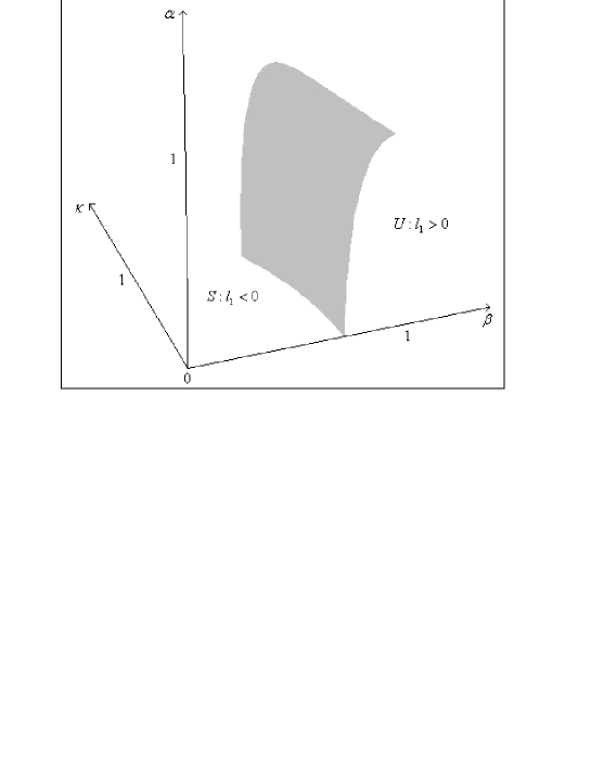
Figure 2: Signs of the first Lyapunov coefficient for system (2.1).

Theorem 4.1

Consider the four-parameter family of differential equations (2.1). The first Lyapunov coefficient at the point (7) for parameter values satisfying (13) is given by

$$l_{1}(\beta,\alpha,\kappa)=-\frac{G_{1}(\beta,\alpha,\kappa)}{4\beta\varepsilon_{c}\omega_{0}^{4}\omega_{1}^{2}(\varepsilon_{c}^{4}+5\varepsilon_{c}^{2}\omega_{0}^{2}+4\omega_{0}^{4})},$$ (35)

where

$$G_{1}(\beta,\alpha,\kappa)=-3+5\kappa\beta-(\alpha^{2}-5)\beta^{2}+\kappa(\alpha^{2}-7)\beta^{3}-$$

$$2\alpha^{2}\kappa^{2}\beta^{4}-(\alpha^{4}-2\alpha^{2}\kappa^{2})\beta^{6}+\alpha^{4}\kappa\beta^{7}.$$ (36)

If $G_{1}$ is different from zero then the system (2.1) has a transversal Hopf point at $P_{0}$ for $\varepsilon=\varepsilon_{c}$. More specifically, if $(\beta,\alpha,\kappa)\in S\cup U$ and $\varepsilon=\varepsilon_{c}$ then the system (2.1) has an H1 point at $P_{0}$; if $(\beta,\alpha,\kappa)\in S$ and $\varepsilon=\varepsilon_{c}$ then the H1 point at $P_{0}$ is asymptotically stable and for each $\varepsilon<\varepsilon_{c}$, but close to $\varepsilon_{c}$, there exists a stable periodic orbit near the unstable equilibrium point $P_{0}$; if $(\beta,\alpha,\kappa)\in U$ and $\varepsilon=\varepsilon_{c}$ then the H1 point at $P_{0}$ is unstable and for each $\varepsilon>\varepsilon_{c}$, but close to $\varepsilon_{c}$, there exists an unstable periodic orbit near the asymptotically stable equilibrium point $P_{0}$. See Fig 2.

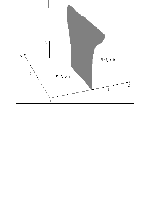
Figure 3: Signs of the second Lyapunov coefficient for system (2.1).

Theorem 4.2

For the four-parameter family of differential equations (2.1) there is unique point $Q=(\beta,\alpha,\kappa,\varepsilon_{c})$, with coordinates

$$\beta=0.93593\ldots,\,\alpha=1.02753\ldots,\kappa=0.90164\ldots,\;\varepsilon_{c}=0.73522\ldots,$$

where the surfaces $l_{1}=0$, $l_{2}=0$ and $l_{3}=0$ on the critical hypersurface intersect and there do it transversally. Moreover, the codimension 4 Hopf point at $P_{0}$ is asymptotically stable since $l_{4}(Q)<0$. More specifically, if $(\beta,\alpha,\kappa)\in S_{1}\cup S_{2}\cup U_{1}$ and $\varepsilon=\varepsilon_{c}$ then the system (2.1) has an H2 point at $P_{0}$; if $(\beta,\alpha,\kappa)\in S_{1}\cup S_{2}$ and $\varepsilon=\varepsilon_{c}$ then the H2 point at $P_{0}$ is asymptotically stable; if $(\beta,\alpha,\kappa)\in U_{1}$ and $\varepsilon=\varepsilon_{c}$ then the H2 point at $P_{0}$ is unstable. Along the curves $C_{1}$ and $C_{2}=C_{21}\cup C_{22}\cup\{Q\}$ of Fig 4 $l_{2}$ vanishes.If $(\beta,\alpha,\kappa)\in C_{1}\cup C_{21}\cup C_{22}$ (see Fig 5) and $\varepsilon=\varepsilon_{c}$ then the four-parameter family of differential equations (2.1) has a transversal Hopf point of codimension 3 at $P_{0}$; if $(\beta,\alpha,\kappa)\in C_{1}\cup C_{22}$ and $\varepsilon=\varepsilon_{c}$ then the H3 point at $P_{0}$ is asymptotically stable and the bifurcation diagram for a typical point $H$ is draw in Fig 6; if $(\beta,\alpha,\kappa)\in C_{21}$ and $\varepsilon=\varepsilon_{c}$ then the H2 point at $P_{0}$ is unstable and the bifurcation diagram for a typical point $G$ can be found in [12].

Computer assisted Proof. The algebraic expression for the second Lyapunov coefficient can be obtained in [16]. This is too long to be put in print. The surface where the second Lyapunov coefficient vanishes is illustrated in Fig. 3.

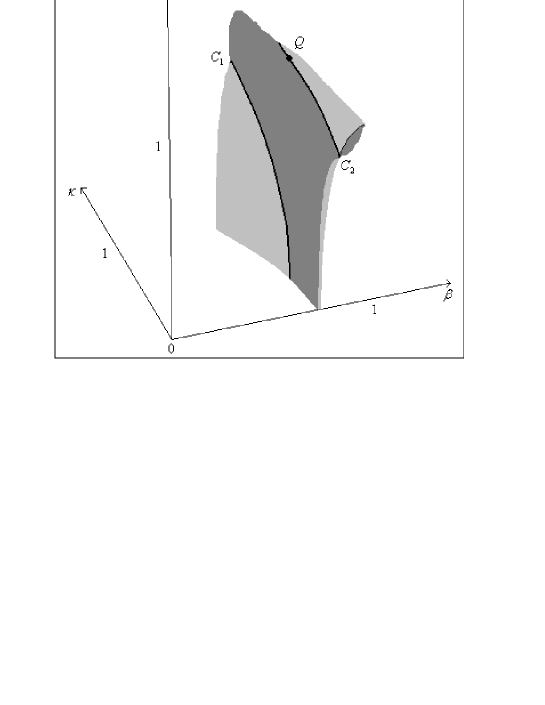
Figure 4: Surfaces $l_{1}=0$ and $l_{2}=0$ and the intersection curves.

The intersections of the surfaces $l_{1}=0$ and $l_{2}=0$ determine the curves $C_{1}$ and $C_{2}$ (see Fig 4). The signs of the second Lyapunov coefficient on the surface $l_{1}=0$ complementary to the curves $C_{1}$ and $C_{2}$, that is on $S_{1}\cup S_{2}\cup U_{1}$ (see Fig. 5), are the following: $l_{2}$ is negative on $S_{1}\cup S_{2}$ and is positive on $U_{1}$ and they can be viewed as extensions of the signs of the second Lyapunov coefficient at points on the curve determined by the intersection of the surface $l_{1}=0$ and the plane $\kappa=0$ studied by the authors in [12]. The bifurcation diagram for a typical point $G$ where $l_{3}(G)>0$ can be viewed in [12]. In Fig 6 and 7 are illustrated the bifurcation diagrams for a typical point $H$ where $l_{3}(H)<0$.

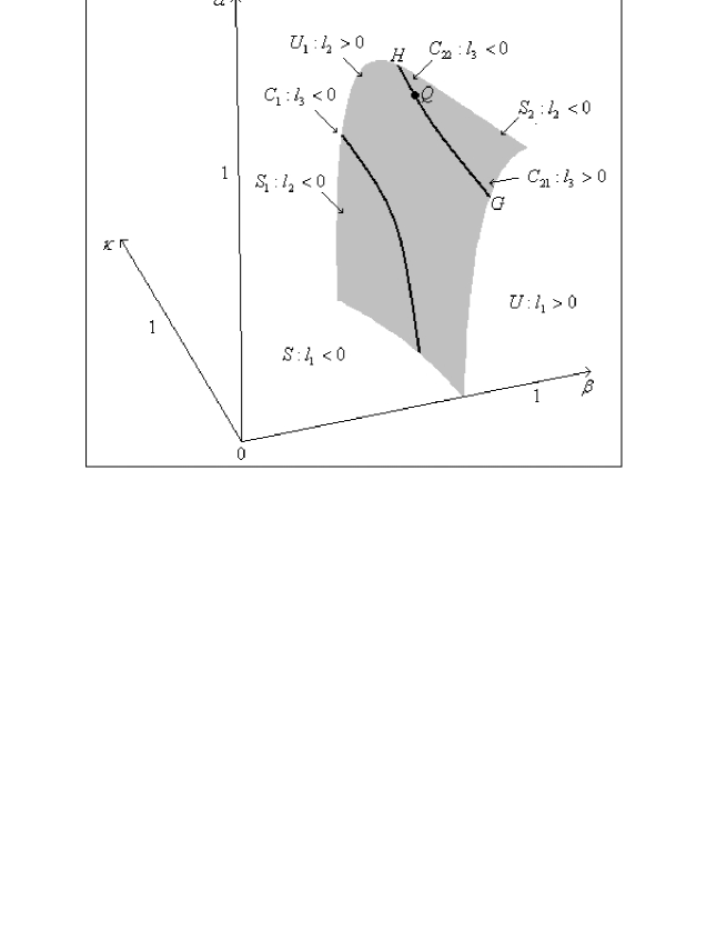
Figure 5: Signs of $l_{1}$, $l_{2}$ and $l_{3}$.

The point $Q$ is the intersection of the surfaces $l_{1}=0$, $l_{2}=0$ and $l_{3}=0$. The existence and uniqueness of $Q$ with the above coordinates has been established numerically with the software MATHEMATICA 5.

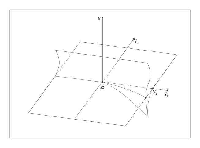
Figure 6: Bifurcation diagram for a typical point $H$ where $l_{3}(H)<0$.

For the point $Q$ take five decimal round-off coordinates $\beta=0.93593$, $\alpha=1.02753$, $\kappa=0.90164$ and $\varepsilon_{c}=0.73522$. For these values of the parameters one has

$$p=\left(-i/2,0.27041-0.54618i,0.40395+0.20000i\right),$$

$$q=\left(-i,0.36401,0.99407\right),$$

$$h_{11}=\left(-2.65769,0,0.19650\right),$$

$$h_{20}=\left(-4.11029-0.18429i,0.13416-2.99241i,0.09159-3.36395i\right),$$

$$h_{30}=\left(-3.63589+23.03616i,-25.15645-3.97054i,-18.16113-1.69167i\right),$$

$$G_{21}=-3.91814i,$$ (37)

$$h_{21}=\left(3.24775+1.67247i,-4.52694+1.18222i,4.85950+3.71541i\right),$$

$$h_{40}=\left(\begin{array}[]{c}160.39204+51.10539i\\ -74.41230+233.53975i\\ -25.03366+127.34049i\end{array}\right),$$

$$h_{31}=\left(-69.44664-38.56274i,25.90851-2.24484i,36.10391-65.85524i\right),$$

$$h_{22}=\left(-64.50829,0,10.76131\right),$$

$$G_{32}=-153.21726i,$$ (38)

$$h_{50}=\left(\begin{array}[]{c}702.48693-1263.93346i\\ 2300.44688+1278.57511i\\ 1054.20770+363.36145i\end{array}\right),$$

$$h_{32}=\left(\begin{array}[]{c}178.24934+273.66781i\\ -233.17715+26.70966i\\ 395.89053+272.77265i\end{array}\right),$$

$$h_{41}=\left(\begin{array}[]{c}-521.71430+1074.26121i\\ -631.58388-484.25803i\\ -865.10385-413.20000i\end{array}\right),$$

$$h_{60}=\left(\begin{array}[]{c}-10130.73267-9995.21750i\\ 21830.38995-22126.36639i\\ 5429.65950-9557.27148i\end{array}\right),$$

$$h_{51}=\left(\begin{array}[]{c}14227.43860+8237.49829i\\ -9991.87299+14431.55078i\\ -5753.08267+11280.54380i\end{array}\right),$$

$$h_{42}=\left(\begin{array}[]{c}-4351.45992-4936.33553i\\ 2272.08822+1527.90723i\\ 4841.97866-5445.36779i\end{array}\right),$$

$$h_{33}=\left(-5969.63958,0,1764.47230\right),$$

$$h_{70}=\left(\begin{array}[]{c}-146941.54096+63522.80004i\\ -161862.28504-374421.36634i\\ -86069.40319-83969.45215i\end{array}\right),$$

$$h_{61}=\left(\begin{array}[]{c}140223.18890-184094.16057i\\ 260780.07852+213929.28545i\\ 151116.49070+92225.27059i\end{array}\right),$$

$$h_{52}=\left(\begin{array}[]{c}-105557.32750+127994.80577i\\ -41289.02476-79039.91108i\\ -106857.14273-88122.45467i\end{array}\right),$$

$$G_{43}=-22328.21224i.$$ (39)

$$h_{43}=\left(\begin{array}[]{c}26579.27090+62051.16515i\\ -36944.56779+2499.10743i\\ 78144.32459+54070.14624i\end{array}\right),$$

$$h_{80}=\left(\begin{array}[]{c}-247681.58290+2173895.03048i\\ -6330624.44741-721276.35507i\\ -1324248.15135+594661.38331i\end{array}\right),$$

$$h_{71}=\left(\begin{array}[]{c}-2230744.30930-2511854.85381i\\ 4663683.99275-4038564.75411i\\ 1618564.33911-2037646.14488i\end{array}\right),$$

$$h_{62}=\left(\begin{array}[]{c}2540059.79128+2277848.86298i\\ -2385453.21697+1869088.06376i\\ -1708253.47087+2025268.53034i\end{array}\right),$$

$$h_{53}=\left(\begin{array}[]{c}-633499.15640-1125590.51413i\\ 390598.08062+466226.40735i\\ 1219484.73373-1101283.41903i\end{array}\right),$$

$$h_{44}=\left(-1118100.12194,0.00138,546721.10946\right),$$

$$G_{54}=-22071.41115-5991090.52119i.$$ (40)

From (28), (30), (32), (34), (37), (38), (39) and (40) one has

$$l_{1}(Q)=0,\>l_{2}(Q)=0,\>l_{3}(Q)=0,\>l_{4}(Q)=\frac{1}{2880}\>{\rm Re}\>G_{54}=-7.66368.$$

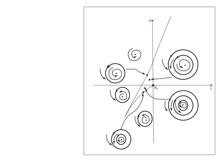
Figure 7: Bifurcation diagram for a typical point $H_{1}$. See Fig. 6.

The calculations above have also been corroborated with 100 decimals round-off precision performed using the software MATHEMATICA 5 [17]. See [16].

Some values of $(\alpha,\beta,\kappa)\in C_{1}\cup C_{2}$ as well as the corresponding values of $l_{3}(\alpha,\beta,\kappa)$ are listed in the tables below. The calculations leading to these values can be found in [16].

$\kappa$	$\alpha$	$\beta$	$l_{3}(\alpha,\beta,\kappa)$ on $C_{1}$
0.45	0.33319	0.72216	-0.91310
0.5	0.42968	0.71770	-0.92567
0.55	0.50934	0.71257	-0.88152
0.6	0.57913	0.70665	-0.82064
0.65	0.64241	0.69983	-0.75810
0.7	0.70113	0.69201	-0.70006
0.75	0.75659	0.68309	-0.64900
0.8	0.80972	0.67302	-0.60580
0.85	0.86120	0.66177	-0.57054
0.9	0.91154	0.64940	-0.54288
0.95	0.96114	0.63600	-0.52217

$\kappa$	$\alpha$	$\beta$	$l_{3}(\alpha,\beta,\kappa)$ on $C_{2}$
0	0.85050	0.86828	0.39050
0.2	0.90524	0.87760	0.46294
0.3	0.93123	0.88397	0.50684
0.4	0.95511	0.89159	0.55538
0.5	0.97602	0.90042	0.60637
0.6	0.99330	0.91029	0.65253
0.7	1.00674	0.92071	0.66963
0.8	1.01697	0.93045	0.56860
0.9	1.02731	0.93592	0.01665
0.92	1.03020	0.93585	-0.20674
0.98	1.04319	0.93201	-1.09289

The gradients of the functions $l_{1}$, $l_{2}$ and $l_{3}$, given in (28), (30), (32) at the point $Q$ are, respectively

$$(-0.46264,0.13437,-0.97565),(-12.44701,2.66791,-19.19345),$$

$$(-266.77145,41.80505,-372.84969).$$

The transversality condition at $Q$ is equivalent to the non-vanishing of the determinant of the matrix whose columns are the above gradient vectors, which is evaluated gives $-33.31133$.

The main steps of the calculations that provide the numerical evidence for this theorem have been posted in [16].

$\blacksquare$

5 Concluding comments

This paper starts reviewing the stability analysis which accounts for the characterization, in the space of parameters, of the structural as well as Lyapunov stability of the equilibrium of the Watt Governor System with a Spring, WGSS. It continues with recounting the extension of the analysis to the first order, codimension one stable points, happening on the complement of a surface in the critical hypersurface where the eigenvalue criterium of Lyapunov holds, as studied by the authors [13], based on the calculation of the first Lyapunov coefficient. Here the bifurcation analysis at the equilibrium point of the WGSS is pushed forward to the calculation of the second, third and fourth Lyapunov coefficients which make possible the determination of the Lyapunov as well as higher order structural stability at the equilibrium point. See also [6, 7], [4] and [2] .

The calculations of these coefficients, being extensive, rely on Computer Algebra and Numerical evaluations carried out with the software MATHEMATICA 5 [17]. In the site [16] have been posted the main steps of the calculations in the form of notebooks for MATHEMATICA 5.

With the analytic and numeric data provided in the analysis performed here, the bifurcation diagrams are established along the points of the surface where the first Lyapunov coefficient vanishes. Pictures 6 and 7 provide a qualitative synthesis of the dynamical conclusions achieved here at the parameter values where the WGSS achieves most complex equilibrium point. A reformulation of these conclusions follow:

There is a “solid tongue” where three stable regimes coexist: one is an equilibrium and the other two are small amplitude periodic orbits, i.e., oscillations.

For parameters inside the “tongue”, this conclusion suggests, a hysteresis explanation for the phenomenon of “hunting” observed in the performance of WGSS in an early stage of the research on its stability conditions. Which attractor represents the actual state of the system will depend on the path along which the parameters evolve to reach their actual values of the parameters under consideration. See Denny [3] for historical comments, where he refers to the term “hunting” to mean an oscillation around an equilibrium going near but not reaching it.

Finally, we would like to stress that although this work ultimately focuses the specific three dimensional, four parameter system of differential equations given by (2.1), the method of analysis and calculations explained in Section 3 can be adapted to the study of other systems with three or more phase variables and depending on four or more parameters.

Acknowledgement: The first and second authors developed this work under the project CNPq Grants 473824/04-3 and 473747/2006-5. The first author is fellow of CNPq and takes part in the project CNPq PADCT 620029/2004-8. The third author is supported by CAPES. This work was finished while the second author visited Universitat Autònoma de Barcelona, supported by CNPq grant 210056/2006-1.

References

[1] A. Al-Humadi and N. D. Kazarinoff, Hopf
bifurcation in the Watt steam engine, Inst. Math. Appl., 21
(1985), 133-136.
[2] A. A. Andronov, E. A. Leontovich et al.,
Theory of Bifurcations of Dynamic Systems on a Plane,
Halsted Press, J. Wiley & Sons, New York, 1973.
[3] M. Denny, Watt steam governor stability, Eur. J.
Phys., 23 (2002), 339-351.
[4] A. Gasull and J. Torregrosa, A new approach to the computation
of the Lyapunov Constants, Comp. and Appl. Math., 20 (2001),
149-177.
[5] B. D. Hassard, N. D. Kazarinoff and Y. H. Wan,
Theory and Applications of Hopf Bifurcation, Cambridge
University Press, Cambridge, 1981.
[6] Y. A. Kuznetsov, Elements of Applied
Bifurcation Theory, Springer-Verlag, New York, 2004.
[7] Y. A. Kuznetsov, Numerical normalization
techniques for all codim 2 bifurcations of equilibria in ODE’s,
SIAM J. Numer. Anal., 36 (1999), 1104-1124.
[8] A. G. J. MacFarlane, The development of
frequency-response methods in automatic control, IEEE T. Automat.
Contr., AC-24 (1979), 250-265.
[9] J. C. Maxwell, On governors, Proc. R. Soc., 16
(1868), 270-283.
[10] L. S. Pontryagin, Ordinary Differential Equations,
Addison-Wesley Publishing Company Inc., Reading, 1962.
[11] J. Sotomayor, L. F. Mello and D. C. Braga, Stability
and Hopf bifurcation in the Watt governor system, Commun. Appl.
Nonlinear Anal. 13 (2006), 4, 1-17.
[12] J. Sotomayor, L. F. Mello and D. C. Braga, Bifurcation Analysis of the
Watt Governor System, Comp. Appl. Math. 26 (2007), 19-44.
[13] J. Sotomayor, L. F. Mello and D. C. Braga, Stability and Hopf Bifurcation
in an Hexagonal Governor System, Nonlinear Anal.: Real World Appl., 9 (2008), 889-898, doi:
10.1016/nonrwa.2007.01.007.
[14] F. Takens, Unfoldings of certain singularities of
vectorfields: Generalized Hopf bifurcations, J. Diff. Equat., 14 (1973), 476-493.
[15] I. A. Vyshnegradskii, Sur la théorie générale des
régulateurs, C. R. Acad. Sci. Paris, 83 (1876), 318-321.
[16] Site with the files used in computer assited
arguments in this work:
http://www.ici.unifei.edu.br/luisfernando/wgss