Water vapour masers in long-period variable stars

Abstract

Context. Water vapour maser emission from late-type stars characterises them as asymptotic-giant-branch stars with oxygen-rich chemistry that are losing mass at a substantial rate. Further conclusions on the properties of the stars, however, are hampered by the strong variability of the emission.

Aims. We wish to understand the reasons for the strong variability of H₂O masers in circumstellar shells of late-type stars. In this paper we study RX Bootis and SV Pegasi as representatives of semiregular variable stars (SRVs).

Methods. We monitored RX Boo and SV Peg in the 22-GHz maser line of water vapour with single-dish telescopes. The monitoring period covered two decades for RX Boo (1987 – 2007) and 12 years for SV Peg (1990 – 1995, 2000 – 2007). In addition, maps were obtained of RX Boo with the Very Large Array over several years.

Results. We find that most of the emission in the circumstellar shell of RX Boo is located in an incomplete ring with an inner radius of 91 mas (15 AU). A velocity gradient is found in a NW–SE direction. The maser region can be modelled as a shell with a thickness of 22 AU, which is only partially filled. The gas crossing time is 16.5 years. The ring-like structure and the velocity gradient remained stable for at least 11 years, while the maser line profiles varied strongly. This suggests that the spatial asymmetry is not accidental, so that either the mass loss process or the maser excitation conditions in RX Boo are not spherically symmetric. The strong variability of the maser spectral features is mainly due to incoherent intensity fluctuations of maser emission spots, which have lifetimes of the order of 1 year. We found no correlation between the optical and the maser variability in either star. The variability properties of the SV Peg masers do not differ substantially from those of RX Boo. There were fewer spectral features present, and the range of variations was narrower. The maser was active on the $>$10-Jy level only 1990 – 1992 and 2006/2007. At other times the maser was either absent ($<$1 Jy) or barely detectable.

Conclusions. The variability of H₂O masers in the SRVs RX Boo and SV Peg is due to the emergence and disappearance of maser clouds with lifetimes of $\sim$1 year. The emission regions do not evenly fill the shell of RX Boo leading to asymmetry in the spatial distribution, which persists at least an order of magnitude longer.

1 Introduction

Water vapour maser emission of the $6_{16}-5_{23}$ transition at1.35-cm wavelength (22 GHz) is often found in the circumstellar shells of oxygen-rich stars on the asymptotic giant branch (AGB) and in several red supergiants (RSGs). The AGB stars have intermediate masses ($M\approx 1-8$ M_⊙) and are usually long-period variables. They encompass semi-regular variables (SRVs), Mira variables and OH/IR stars. The classification of SRVs and Mira variables is made in the optical regime and they are distinguished by the amplitude of their intensity variations. Due to their higher mass-loss rates OH/IR stars are optically faint and their variability is observed in the infrared (see review by Habing Habing96 (1996)).

SRV, Mira and OH/IR stars form a sequence of increasing mass-loss rates, but it is not clear if this is also an evolutionary sequence or a sequence of increasing progenitor masses. RSGs are stars with masses $M>$ 8 M_⊙ in a short evolutionary phase, where mass-loss rates are high and they develop circumstellar dust and gas shells as AGB stars do.

Immediately after the discovery of H₂O masers in the envelope of the RSG VY CMa, variability was noticed (Knowles et al. Knowles69 (1969); Buhl et al. Buhl69 (1969)). From monitoring observations of AGB stars and RSGs (Schwartz et al. Schwartz74 (1974)) evidence was found that the observed maser spectra varied in peak and integrated flux, in line profiles and possibly in line-of-sight velocity (Dickinson et al. Dickinson73 (1973)). The earliest studies of long-period variables found that the maser variability was well correlated with variations in the optical and in the infrared (Schwartz et al. Schwartz74 (1974)), but later observations showed that the regularity of the radio variations had been overestimated (Engels et al. Engels88 (1988); Cohen Cohen89 (1989)). The first interferometric maps of the Mira variables R Aql and RR Aql taken at two epochs separated by 15 months also showed dramatic changes (Johnston et al. Johnston85 (1985)). Knowledge of the properties of the variability and understanding of the reasons for it, however, are prerequisites for the interpretation of the observations and for the derivation of basic stellar properties.

Water vapour masers are potentially very sensitive tools to probe the physics and dynamics in parts of the circumstellar shells, whose radii range between $\sim$5 and 50 AU in case of Mira variables and SRVs (Bowers et al. Bowers93 (1993); Bowers & Johnston Bowers94 (1994); Colomer et al. Colomer00 (2000); Bains et al. Bains03 (2003); Imai et al. Imai03 (2003)). High-resolution mapping with interferometers shows that the integrated maser emission is composed of a multitude of individual clouds of sizes $\sim$2 – 4 AU and a low filling factor of $\sim$0.01 (Bains et al. Bains03 (2003)). In conjunction with the SiO masers located closer to the central star and with the OH masers in the outer parts of the envelope, H₂O masers allow us to map the shell that is created by the strong mass loss ($>$$10^{-7}$ $M_{\sun}$ yr^-1) on the upper AGB. Information on the velocities and on the distribution of the maser spots can be used to reconstruct the geometry of the mass-loss process and sometimes even its history.

Monitoring of H₂O maser emission with single-dish radio telescopes, even covering more than a decade, provides only limited insight. The spectra mostly consist of many components, which often overlap in velocity. The profiles and intensities of H₂O maser spectra therefore depend not only on temperature variations due to the pulsating star but also on other factors, including random intensity fluctuations of individual clouds (Engels et al. Engels88 (1988)). Early programmes followed only the strongest lines. Three years of monitoring led Cox & Parker (Cox79 (1979)) to the conclusion that the masers are not stable for more than a few pulsation cycles. Later Little-Marenin and co-workers monitored a few Mira variables over a number of years and found complex variations in intensity with many components varying independently from one another (e.g. Little-Marenin et al. Little91 (1991)). Usually a phase lag of $\sim$0.3 (30 – 100 days) with respect to the visual maximum was observed (Little-Marenin et al. Little93 (1993)). A Russian group monitored a number of stars with strong H₂O masers for up to twenty years. They found that by and large the maser flux correlates with the visual light curve, and confirmed the presence of a phase lag. They attributed the maser variations and the phase lag to the passage of periodic shocks (Lekht et al. Lekht05 (2001), and references therein).

Table 1: The VLA observing schedule

Date	Conf.	Sources
1990 Feb. 26	A	RX Boo, U Her, OH 39.7+1.5,
		OH 83.4$-$0.9, VX Sgr
1990 June 3	A	RX Boo, U Her, OH 39.7+1.5,
		OH 83.4$-$0.9, VX Sgr
1991 Aug. 23	A	OH 39.7+1.5
1991 Oct. 20	BnA	RX Boo, U Her
1992 Jan. 10	B	VX Sgr, NML Cyg
1992 Dec. 28	A	RX Boo, U Her, OH 39.7+1.5
1995 Sept. 5	A	RX Boo
1996 Dec. 10	A	OH 26.5+0.6
1998 May 31	A	OH 26.5+0.6

In order to improve the understanding of the properties of maser variability for different types of late-type stars, we started in 1987 a monitoring programme of several such stars using the Effelsberg and Medicina radio telescopes. The sample included SRVs, Mira variables, OH/IR stars and RSGs. In order to break the spatial degeneracy, which usually makes the interpretation of single-dish maser spectra difficult, we added interferometric observations using the Very Large Array (VLA). Of each object type we selected prototypical stars, which were observed during several epochs (see Table 1). In this paper we present the results for two SRVs: RX Bootis (RX Boo) and SV Pegasi (SV Peg). In subsequent papers we will present results for the other types of late-type stars.

RX~Boo is a 9 – 11 mag SRV with a mean spectral type of M7.5 and a period varying between 340 and 400 days (Kukarkin et al. Kukarkin71 (1971)). Olofsson et al. (Olofsson02 (2002)) in their model fit involving several CO transitions estimated a mass-loss rate of 6  $\times$ $10^{-7}$ $M_{\sun}$ yr^-1 and an expansion velocity of 9.3 km s^-1 , whereas Teyssier et al. (Teyssier06 (2006)), as a result of another model fit, obtained 2  $\times$ $10^{-7}$ $M_{\sun}$ yr^-1 and 7.5 km s^-1, respectively. The distance is 160$\pm$25 pc (The Hipparcos Catalogue; Perryman et al. Perryman97 (1997)). Dyck et al. (Dyck95 (1995)), using an IR interferometer, measured the stellar diameter at 2.2  $\mu$m and found a uniform-disk (UD) diameter of 19$\pm$1 mas. They calculated an effective temperature of 3000 $\pm$ 100 K. Chagnon et al. (Chagnon02 (2002)), observing in a band centred at 3.8 $\mu$m, found a UD diameter of 21.0 $\pm$ 0.3 mas.

The H₂O maser of RX Boo is one of the first masers of this kind detected in late-type stars (Schwartz & Barrett Schwartz71 (1971); Dickinson et al. Dickinson73 (1973)), and hence it is one of the best studied. Single-dish monitoring was performed by Schwartz et al. (Schwartz74 (1974)), Cox & Parker (Cox79 (1979)), Berulis et al. (Berulis83 (1983)), and Hedden et al. (Hedden91 (1991)) who all found a weak correlation of maser intensity with optical flux. Maps taken with the VLA show an overall extent of the maser shell of 150 – 230 mas (Bowers et al. Bowers93 (1993); Colomer et al. Colomer00 (2000)), giving an outer shell radius of 12 – 18 AU or 9 – 14 stellar radii.

SV~Peg also varies with $\sim$2 mag amplitude (9 – 11 mag) and has a spectral type of M7 and a mean period of 144 days (Kukarkin et al. Kukarkin71 (1971)). The mass-loss rate is 3  $\times$ $10^{-7}$ $M_{\sun}$ yr^-1 at an expansion velocity of 7.5 km s^-1 (Olofsson et al. Olofsson02 (2002)) and its distance is 205$\pm$45 pc (The Hipparcos Catalogue; Perryman et al. Perryman97 (1997)). The H₂O maser was discovered by Dickinson (Dickinson76 (1976)) and was only occasionally observed before our monitoring efforts. No mapping has been done as yet.

2 Observations

Single-dish observations of the H₂O maser line at 22235.08 MHz were made with the Effelsberg 100-m and Medicina 32-m telescopes at typical intervals of a few months. RX Boo was monitored over twenty years between 1987 and 2007, and SV Peg in 1990 – 1995 and 2000 – 2007. VLA observations were made of RX Boo on four occasions in the period 1990 – 1992 and later in 1995 after a strong flare event (see Table 1). This event will be discussed in a separate paper.

2.1 Effelsberg observations

With the 100-m telescope observations were made of RX Boo between 1990 February and 2002 June and of SV Peg between 1990 February and 1995 June. We used the 18 – 26-GHz receiver to observe the $6_{16}\rightarrow 5_{23}$ transition of the water molecule. The receiver had a cooled maser as pre-amplifier and passed left-hand circularly polarised radiation. As circumstellar water masers are found to be unpolarised to limits of a few percent (Barvainis & Deguchi Barvainis89 (1989)), significant flux losses due to the polarization properties of the receiver are not expected. At 1.3-cm wavelength the beamwidth is $\sim$40″ (FWHM). We observed in total power mode integrating ON and OFF the source for 5 min each. ‘ON-source’ the telescope was positioned on RX Boo at the coordinates $\alpha=14^{\rm{h}}\,24^{\rm{m}}\,11\aas@@fstack{s}6$, $\delta=+25\degr\,42\arcmin\,13\arcsec$ (J2000) and on SV Peg at $\alpha=22^{\rm{h}}\,05^{\rm{m}}\,42\aas@@fstack{s}1$, $\delta=+35\degr\,20\arcmin\,54\arcsec$ (J2000), while the ‘OFF-source’ position was displaced 3′ to the east of the source. Typical system temperatures were 60 – 120 K depending on weather conditions and elevation. The typical rms noise-level in the spectra is $\sim$0.2 Jy.

The backend consisted of a 1024-channel autocorrelator. Observations were made with a bandwidth of 6.25 MHz, centred on the systemic line-of-sight velocity of the star. The velocity coverage was $\sim$80 km s^-1 and the velocity resolution 0.08 km s^-1.

Standard procedures were used to reduce the spectra. First a baseline was fitted using the channels not affected by emission, then the calibration was applied. Finally, spectra from several integrations of the same source were averaged, if they were taken during the same day. Hanning smoothing to 0.16 km s^-1  was applied only to noisy spectra.

The flux calibrations were made against NGC 7027 (5.9 Jy) and Mon R2 (6 Jy), and corrections for atmospheric attenuation and elevation were applied using a standard gain curve determined under good weather conditions. Deviations from the standard gain curve were less than 10%, except at low elevations where deviations up to 30% were measured. Losses due to pointing are at most secondary effects, as pointing checks and corrections were regularly carried out on strong continuum sources, showing deviations from the nominal position of at most 10″.

2.2 Medicina observations

Observations at Medicina were carried out between 1987 March and 2007 January on RX Boo and between 1990 February and 1995 January and again between 2000 October and 2007 January on SV Peg. The Medicina 32-m telescope (HPBW at 22 GHz $\sim 1$.^′9) is set up primarily to be used for VLBI measurements, and therefore the front-end is typical for such work. For line observations at 22 GHz only the right-hand circular polarization output from the receiver is available.

Over the years the system has undergone various improvements. In 1989 realignement of the antenna surface resulted in an improvement of the efficiency at 22 GHz from 17 to 38%. The backend was a 512-channel digital autocorrelator; in 1991 the number of channels was increased to 1024. In the same year a HEMT amplifier replaced the GaAs FET front-end, reducing the system temperature (120 K at zenith under good weather conditions). Also in 1991 an active sub-reflector control increased the gain at low and high elevations. The available bandwidth varied between 3.125 MHz and 25 MHz. Up to 1997 the spectral resolutions used corresponded to 0.082 km s^-1 or 0.165 km s^-1. In 1997 the VLA-1 chip correlator was replaced by one based on the NFRA correlator chips and boards (Bos Bos91 (1991)); in the standard configuration the latter has 2048 channels and a maximum bandwidth of 160 MHz. However, to maintain consistency with the older observations we have only used a 10 MHz band and 1024 channels, giving a velocity resolution of 0.132 km s^-1.

The telescope pointing model is typically updated a few times per year, and is quickly checked every few weeks by observing strong maser sources (e.g. W3 OH, Orion-KL, W49 N, and/or Sgr B2 and W51). The pointing accuracy was always better than 25″; from about mid 2004 the rms residuals from the pointing model were of the order of $8$″$-10$″. The antenna gain as a function of elevation was determined by daily observations of the continuum source DR 21 at a range of elevations; we assume a flux density of 16.4 Jy (after scaling the value of 17.04 Jy given by Ott et al. (Ott94 (1994)) for the ratio of the source size to the Medicina beam). The daily gain curve was determined by fitting a polynomial to the data, which was then used to convert antenna temperature to flux density for all spectra taken that day. From the dispersion of the single measurements around the curve we find the typical calibration uncertainty to be 19%. On the few days that no separate gain curve was measured, we have applied the one closest in date, and estimate a corresponding calibration uncertainty of 7%. The average overall calibration uncertainty is therefore estimated at $\sim$20%.

Observations were taken in total power mode, with both ON and OFF scans of 5-min duration. The OFF position was taken 1° W of the source position. Typically, 2 ON/OFF pairs were taken. The typical rms noise-level in the spectra is $\sim$1.5 Jy. Finally, no observations were taken between 1996 April and 1997 February, due to extensive maintenance work on the telescope.

For the purpose of studying the long-term variability of the maser emission, spectra of the same source taken less than 4 days apart were averaged. During the period that the sources were also monitored at Effelsberg it may happen that we have spectra from both telescopes within 4 days. In these cases we always used the Effelsberg spectra because of their much lower noise level. With very few exceptions both spectra showed the same line profile and flux densities (within 10%) of the individual emission components, providing an a posteriori check on the correctness of the calibration procedures of both telescopes.

2.3 VLA observations

Table 2: VLA map specifications for RX Boo

Date	HPBW			rms	$S/N$
	maj.a.	min.a.	p. a.
	(″)	(″)	(°)	(Jy/b.)
1990 Feb.	0.090	0.077	86.23	0.015	3700
1990 June	0.082	0.078	40.12	0.014	1700
1991 Oct.	0.305	0.092	$-76.62$	0.025	190
1992 Dec.	0.077	0.072	$-23.67$	0.027	130
1995 Sep.	0.127	0.084	$-67.27$	0.009	580

maj.a.: half-power beam width (HPBW) for the major axis of the best-fit three-dimensional Gaussian component to the synthesised beam
min.a.: HPBW for the minor axis
p.a.: position angle of the major axis (E of N)
rms: the root-mean-square noise fluctuations in signal-free channels in units of Jansky per beam area
S/N: signal-to-noise ratio or ‘dynamic range’ in the channel with strongest signal

RX Boo was observed with the VLA on four occasions between 1990 February and 1992 December (Table 1). An additional observation was made in 1995 September after the occurrence of a strong flare, which will be discussed in a separate paper. All 27 antennas were used yielding synthesised beamwidths as specified in Table 2. These beamwidths depend mainly on the configuration, i.e. the extent of the array. For three of the four epochs we used the largest extent (A; see Table 1), while the October 1991 observations were carried out with a hybrid configuration (BnA).

We chose a receiver bandwidth of 3.125 MHz to obtain a total velocity range of 42 km s^-1 and the bandwidth was split into 64 channels, yielding a velocity resolution of 0.66 km s^-1. Data from the right and left circular polarization modes were averaged. Typical integration times were 30 min on the star and 12 min on the phase calibrator J1407+284 with a sampling time of 30 sec. Flux calibration was obtained relative to 3C286 that was assumed to have a flux density of 2.55 Jy and 3C84 was used to correct for the bandpass shapes.

Figure 1: Sample H₂O maser spectra of RX Boo showing typical profiles starting in 1987 and ending in early 2007. Note the varying flux density scale.

The data were reduced with AIPS (Astronomical Image Processing System) using the spectral line data routines. To improve the sensitivity as well as the dynamic range, self-calibration was applied. Care was taken to select an unresolved feature as phase reference. It turned out that bright features often are extended and we made several trials to find the best unresolved feature. Usually we used a point source model for the first iteration. The final sensitivity reached on line-free channels was 9 – 27 mJy/beam depending on weather conditions and integration time (see Table 2).

3 Single dish data of RX Boo

3.1 Definitions

To interpret the single dish maser profiles we will use several terms, whose definitions are given here. The integrated maser emission from a circumstellar shell is a superposition of emissions arising from many physical entities (maser clouds). These emissions are in the form of narrow maser lines, which emit at the velocity of the cloud projected on the line-of-sight. Observed with a single radio telescope all the maser lines together form a maser spectrum with usually several peaks. The shape of the often contiguous spectrum is named maser profile. The data analysis aims at a decomposition of the spectrum into individual maser lines. However, due to blending in velocity space, the analysis rarely results in individual lines but in maser features, which are composed of two or more maser lines. These maser features might be traced over some period of time in several spectra and may reappear at later times perhaps with a slightly different velocity ($\la 0.5$ km s^-1). They might be identified with real maser clouds persisting over this period of time. However, most likely the features are composed of several real clouds with velocities close to one another but spatially separated. We will use the interferometric maps to identify these (groups of) maser clouds, which we name more generally maser spatial components. For accounting purposes all spectral features were grouped according to their velocities into maser spectral components. At different times within the monitoring period of 20 years different spectral features contribute to a spectral component, reflecting the asynchronous formation and dissolution of the contributing maser clouds.

3.2 H₂O maser spectra

Our monitoring of RX Boo covers almost 21 years, from 1987 March to 2007 January with several (typically 4 – 5) observations per year. Depending on telescope (i.e. Effelsberg or Medicina), date of observation and integration time the rms sensitivity of the observations was very inhomogeneous ranging from 0.1 to 6 Jy. All spectra taken are shown in the Appendix (Fig. A1). Sample spectra showing typical profiles are given in Fig. 1. A general view on the properties of the masers and their variations is given in Fig. 2. Here the spectra are arranged along a time axis and the flux densities in between observations are interpolated to obtain an approximated continuous variability profile.

The H₂O masers of RX Boo covered a constant velocity interval between –5 and +5 km s^-1, although at particular velocities the maser emission could drop below the detection threshold for extended periods of time (months to even years). In the time range 1987 – 1989 ($t\la 1000$ in Fig. 2) RX Boo displayed a strong maser feature at 2.5 km s^-1 reaching flux density levels of a few hundred Janskys. In 1995 ($t\sim 2900$) a flare was observed at a velocity of 3.4 km s^-1 with a peak flux density of $>$1500 Jy. During the rest of the time typical flux density levels were $<$100 Jy. The maser never completely disappeared, although occasionally the flux density of the strongest emission peak was only a few Janskys.

Although strong flux variations were observed, leading to a great variety of spectral profiles, they did not occur at random velocities within the observed velocity interval. With a few exceptions the emission at $v_{\rm los}>0$ km s^-1(observed line-of-sight velocity) was always stronger than that at $v_{\rm los}<0$ km s^-1, with the strongest peak occurring between 1.5 and 3.5 km s^-1.

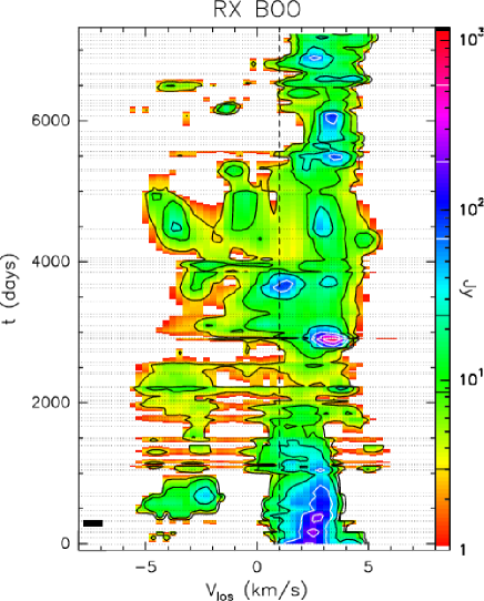
Figure 2: Flux density of the H₂O masers of RX Boo as a function of velocity and time. The time axis covers the years 1987 – 2007. The time stamp $t=0$ corresponds to 1987 March 30 (J.D. 2446885). The dotted horizontal lines mark the actual observations averaged in 4-day intervals. Flux densities in between the observations were interpolated linearly. The spectra were resampled to a resolution of 0.3 km s^-1. The dashed vertical line marks the stellar systemic velocity (1 km s^-1) as given by Teyssier et al. (Teyssier06 (2006)). Contours are drawn at levels 3.00, 8.49, 24.03, 68.02, 192.51, 544.85 Jy (logarithmic scale). These six levels are indicated by black and white lines in the flux scale along the right side of the map. (For a colour version of this figure, see the electronic edition.)

3.3 Line profile analysis

The H₂O maser spectra of RX Boo were decomposed into separate features by fitting multiple Gaussian line profiles. We generally used an iterative procedure in which we first fitted and subtracted the strongest features in each spectrum and then extracted the weaker features from the residual spectrum. The number of extracted features depended on the quality of the spectra as well as the number of distinct peaks. Blending of maser lines is a major obstacle and the extracted features may consist of two or more lines. Depending on the strength of the contributing lines the central velocity of the extracted feature may vary. As a rule of thumb, the FWHM of strong features (visible as distinct peaks in the spectra) is $\sim$1 km s^-1, and therefore features with FWHM $\ga$ 2 km s^-1 are most probably blends. Comparison with adjacent spectra often shows that blended features split when the relative intensities of the contributing lines change. In complex situations when Gaussian fitting failed, features were identified by eye and velocities and flux densities measured by hand. We assumed that maser features in adjacent spectra with velocity differences $\la$0.5 km s^-1 belong to a unique spatial maser component in the shell of RX Boo, which varied in intensity with time. All features were accordingly assigned to 11 maser spectral components labeled A, B,…, K. These components are listed in Tables A and A in the Appendix. For each spectrum we give the Gregorian and Julian dates, its rms noise level in Jansky, the $S_{\rm{I}}$ in $10^{-22}$ W m^-2, and the velocities ($v_{\rm{p}}$) and peak flux densities ($S_{\rm{p}}$) for each component. Occasionally, features were considered as blends and were assigned to two or more components. Values marked by “:” and upper limits were measured with the cursor on the computer screen.

3.4 Line fitting results

Tables A and A show that the maser features at $v_{\rm los}<$ 0 km s^-1 were weaker than those at $v_{\rm los}>$ 0 km s^-1 over the full monitoring period. One spectral component, C, at –2.7 km s^-1, was detected at almost every epoch, whilst A, B, D and E were only detected sporadically. This may be largely a sensitivity effect, because many spectra did not have a sufficient signal-to-noise ratio to allow detection of the fainter features on the level of a few Janskys. In the red part of the maser profile ($v_{\rm los}>$ 0 km s^-1) heavier blending of lines made the unambiguous assignment of features to the components F – K a non-trivial task (Table A). The features assigned to component I, for example, show a systematic velocity shift with $v_{\rm{p}}$$=+2.7\pm 0.3$ km s^-1 until 1992 and $+3.2\pm 0.3$ km s^-1 after 1994. Most likely the emission contributing to component I came from (at least) two maser clouds, of which one of them dominated the emission during the first time range and the other one during the second time range. Similar shifts are observed among the other spectral components. The direction of the shifts does not show any systematics so that we regard these shifts generally as a result of blending by two or more maser lines contributing to a spectral component. Some components show a rather large scatter of velocities, as for example component G with 0.4 $\leq$ $v_{\rm{p}}$$\leq$ 1.9 km s^-1. These “shifts” are almost random and are also not well explained as movements of a physical maser cloud, but rather as a result of blending of several maser lines in the velocity interval 0 – 2 km s^-1 and varying relative intensities. The spectral components F and G show therefore some overlap in velocity, indicating that they are not well defined. Spatial resolution of the maser emission is required to overcome the limited interpretational power of the single dish maser profiles.

However, it is obvious from Fig. 2 as well as from the run of velocities in individual spectral components (Tables A and A) that the lifetimes of individual components are limited on the scale of months up to a few years. The lifetimes will be addressed in more detail in Sect. 4.5.

Figure 3: Sample H₂O maser images of RX Boo from 1990 February. Each image is separated from its neighbours by the line-of-sight velocity interval 0.658 km s^-1. The synthesised FWHM beam size (major axis: 0.^′′09; minor axis: 0.^′′08; position angle of the major axis: 86°) is shown in the uppermost left image (7.9 km s^-1). The images are oriented along right ascension and declination and the angular scales are relative to the position $\alpha=14^{\rm{h}}\,24^{\rm{m}}\,11\aas@@fstack{s}6$, $\delta=+25\degr\,42\arcmin\,14\arcsec$ (J2000). Brightness contours are -0.05 (dashed contour), 0.05, 0.5, 5, 50 Jy per beam area (1.45 $10^{-13}$ sr).

4 Interferometric data of RX Boo

Interferometric observations of the maser emission aim at mapping the maser clouds and breaking the spatial degeneracy. Due to the limited spatial resolution of the instrument this may be only partially successful, and the data analysis of the images will yield maser spatial components, which will be superpositions of several maser clouds close to each other in space as well as in velocity.

4.1 Channel-map analysis

The VLA interferometric data consist of one data cube for each of the four observations, containing 63 maps each. The maps are separated in velocity by 0.658 km s^-1. An example is given in Fig. 3 where maps of the 22 channels with detected signal are displayed from the first VLA epoch (1990 February). Except for the central velocity range the maser emission consists of point-like and unresolved spots. In order to single out maser components the data cubes were analyzed within AIPS in a three step process. First, the individual channel maps were analyzed one by one, then components were identified by comparing neighbouring channel maps, and finally these components were verified in velocity space.

The analysis of the channel maps was made by fitting up to four two-dimensional Gaussian components with elliptical cross sections to the emission spots. The results of this analysis tend to be insecure as soon as spots are blended spatially as well as in velocity. The positions of the fitted Gaussian components are obtained with an accuracy of $\sim$0.02 pixel (0.4 mas) for strong emission spots ($>$1 Jy). Comparing the positions of such spots extending over several channels yields deviations $\leq$0.2 pixel ($\leq$4 mas) between the positions of the same spot in different channel maps. The positions of fainter emission spots have errors up to 0.5 pixel (0.^′′01). Very faint spots ($\leq$300 mJy) can be localised by summing over several channels, usually three. This is guided by the experience that spatial components extend in velocity by not more than $\sim$3 channels ($\sim$2 km s^-1). Often the Gaussian components fitted to weak spots from merged channel maps tend to be extended, indicating that these spots are actually blends of several weak emission spots. Due to high signal-to-noise ratios the positional accuracy obtained from Gaussian fits is much better than the resolution of the interferometer of $\sim$4 pixel (FWHM $\sim$ 0.^′′08), allowing us to determine the relative spatial separation of spots down to 4 – 10 mas.

Table 3: Spatial and spectral components of RX Boo

Spat.	Date	Vel.	Flux	Xoff	Yoff	Spec.
C.		[km/s]	[Jy]	[mas]	[mas]	C.
A1	Feb. 90	$-$4.5	1.5	$-$40	+84	A
A1	Jun. 90	$-$4.5	0.9	$-$37	+68
A1	Oct. 91	$-$5.1	0.7	$-$38	+84
A1	Dec. 92	$-$4.8	0.6	$-$62	+66
A2	Feb. 90	$-$4.5	1.5	$-$27	+151
A2	Jun. 90	$-$4.5	1.5	$-$33	+140
A2	Oct. 91	$-$4.5	1.6	$-$34	+146
A2	Dec. 92	$-$4.2	0.5	$-$58	+126
B1	Dec. 92	$-$3.8	3.5	$-$6	+90	B
C1	Feb. 90	$-$3.2	6.0	+28	+81	C
C1	Jun. 90	$-$3.2	2.0	+21	+72
C2	Feb. 90	$-$3.2	0.5	$-$36	+105
C2	Jun. 90	$-$3.8	0.3	$-$41	+106
C3	Oct. 91	$-$2.5	4.2	$-$18	+92
C3	Dec. 92	$-$2.5	1.0	$-$42	+92
C4	Dec. 92	$-$2.5	0.7	+20	+60
D1	Dec. 92	$-$2.2	0.7	$-$86	+16	D
D2	Jun. 90	$-$1.9	0.6	$-$9	+90
E1	Oct. 91	$-$0.9	1.5	$-$12	+94	E
E1	Dec. 92	$-$1.2	0.8	+48	+64
F1	Feb. 90	$-$0.5	1.0	$-$80	$-$35	F
F1	Jun. 90	$-$0.5	0.3	$-$77	+62
F2	Feb. 90	+0.1	1.0	+29	+116
F2	Jun. 90	+0.1	3.0	+39	+134
F2	Dec. 92	$-$0.2	0.4	+6	+106
F3	Dec. 92	+0.4	1.5	+78	+88
G1	Feb. 90	+0.1	12.0	+81	$-$46	G
G1	Jun. 90	+0.1	5.0	+83	$-$55
G1	Oct. 91	+0.8	5.2	+86	$-$55
G1	Dec. 92	+0.8	0.4	+84	$-$65
G2	Oct. 91	+1.1	4.0	+4	+92
H1	Feb. 90	+1.4	18.0	+58	+154	H
H1	Jun. 90	+1.4	18.0	+55	+148
H1	Oct. 91	+2.1	5.8	+66	+158
H1	Dec. 92	+2.1	2.8	+68	+168
H2	Feb. 90	+1.4	0.5	$-$80	+74
H2	Jun. 90	+1.4	1.3	$-$81	+64
H3	Feb. 90	+2.1	10.0	+97	+10
H3	Jun. 90	+1.4	8.0	+99	$-$7
H3	Dec. 92	+2.1	1.2	+70	+58
H4	Dec. 92	+2.1	0.2	+80	$-$59
I1	Feb. 90	+2.8	70.0	+100	+34	I
I1	Jun. 90	+2.8	26.0	+99	+26
I2	Feb. 90	+3.4	5.0	+88	+14
I2	Oct. 91	+2.4	3.8	+88	+18
I3	Dec. 92	+3.4	0.1	$-$44	+164
J1	Oct. 91	+4.4	5.3	+66	+50	J
J1	Dec. 92	+3.7	2.3	+76	+58
K1	Feb. 90	+4.7	8.5	+59	+99	K
K1	Jun. 90	+4.7	1.4	+51	+30
K2	Jun. 90	+6.0	0.6	+47	+34

4.2 Spatial component identification

Subsequently, neighbouring channel maps were compared and spatial maser components were identified by looking for spatially coincident Gaussian components. Spatial maser components were accepted as real, if they had Gaussian components in at least two neighbouring channel maps. Gaussian components present in only one map are always weak, and are not considered further. They might be real maser components but cannot be verified. At last we made sure that the list of identified spatial maser components can be identified also in velocity space. For this purpose ‘slices’ along the velocity axis through the cube were obtained at the spatial positions of the components. Usually the components stand out as distinct peaks in these ‘slices’, confirming their reality. Spatial components blended in velocity by another strong component, reveal themselves by adding considerable asymmetry to the velocity profile of the major component. Asymmetric velocity profiles of components is a strong indication of blending and may reveal new components that are separated marginally in velocity but not spatially within the resolution of the maps. The final list of components consists of all components verified spatially as well as in velocity

Typically 10 to 15 spatial maser components were identified in each VLA observing epoch. These components are listed in Table 3. For the epoch 1990 June the components can be compared to those found by Colomer et al. (Colomer00 (2000)), who used the VLA to observe RX Boo one day apart from our observation. To determine the spatial components they used a 3-D Gaussian fitting programme developed to analyze directly the spectral data cubes. They find about the same number of components (15 vs. 14), and their Gaussian-fitted intensities and the overall spatial distribution of their components are compatible with our results. The rms scatter in intensities and positions for components in common are 2 Jy and 30 mas, respectively. The positional deviations are a factor $>$3 higher than the relative positional accurary of 4 – 10 mas derived above. A possible cause for the scatter is the extensions of the maser clouds. Bains et al. (Bains03 (2003)) found sizes of 2 – 4 AU for the Mira stars U Ori and U Her. Adopting these sizes for RX Boo, angular sizes of $\sim$40 mas are predicted, much larger than the implied positional accuracies from the Gaussian fits. We suspect that the two fitting methods treat the effect of blending of the extended maser clouds differently, spatially as well as kinematically.

To search for continuum emission of the star we formed the average of all channels without line emission, yielding rms fluctuations of the order of 5 mJy/beam. The non-detection is in agreement with the expected blackbody flux density of $\sim$0.3 mJy from a star with a diameter of 19 mas and a photospheric temperature of 3000 K.

4.3 Alignment of the maps

In order to identify spatial components present over two or more observing epochs we aligned the four maps to a common origin. The maps of 1990 were very similar showing the majority of components to be present in both maps and making the alignment trivial. Several spatial components in common were found also in the 1991 and 1992 maps, however, the components in common with the 1990 maps were scarce. Finally, we chose the strong spatial components G1, H1 and I1/I2 (see Table 3) to obtain an alignment of all four maps. After alignment these components scattered in position by $\sim$10 mas.

Spatial coincidences among the weaker components were searched for in the aligned maps. After subtraction of coincident components we ended up with 25 different spatial components of which 64% were present in at least two maps. Positional deviations between maps were typically of the order of 30 mas, although in a few ambiguous cases we accepted as coincidences also components with deviations up to 60 mas (cf. E1, H3, K1 in Table 3). The velocity and spatial resolutions were clearly insufficient to avoid such ambiguities.

According to their velocity, the merged spatial components were assigned to the eleven spectral components A…K. The merged components are listed in Table 3, which gives the spatial component (Spat. C.), the VLA observing epoch, the line-of-sight velocity and peak flux of the spatial component identified, the spatial offsets (Xoff and Yoff) from the adopted map centre (see below) and the associated spectral component (Spec. C.) from Tables A and A in the Appendix.

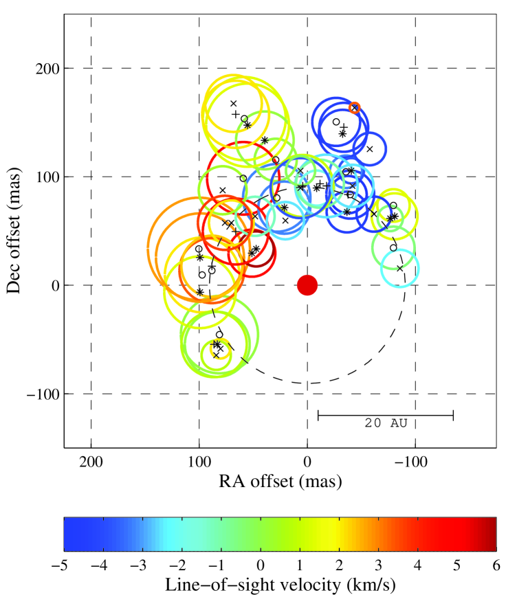
Figure 4: All the maser components listed in Table 3 plotted on the sky. Each component is represented by a symbol and a circle whose diameter is logarithmically proportional to the flux density of the component (see text for the mathematical expression). The epochs are represented by different symbols: 1990 February by small circles; 1990 June by asterisks; 1991 October by plus signs; 1992 December by crosses. The circles around the components are colour coded according to the line-of-sight velocity of the component ($v_{\rm los}$ in the text). (For a colour version of this figure, see the electronic edition.) A circle (dashed) has been fitted to the components on the arc (see text for a detailed list of components) and the origin has been moved to the centre of this circle (Table 3). The filled dark red circle at the origin symbolises the central star with a diameter of 19 mas.

4.4 Distribution of spatial components

The distribution of spatial components from all maps after alignment is shown in Fig. 4. The flux density of the spatial components is represented by the sizes of circles centred on the position of the components. Due to the large range in flux (see the third column of Table 3) we have chosen a logarithmic relation:

$$d=20\,{\rm log}\,S+26$$ (1)

where $d$ is the diameter of the circle in milliarcseconds and $S$ is the flux density in Janskys.

In this map the most prominent feature is the incomplete ring-like structure where most of the spatial components reside. The south-western part of the ring contained no emission during all four observing epochs covering 3 years. The second obvious feature is a velocity gradient with most of the redshifted emission ($v_{\rm los}>2$ km s^-1) located in the south-eastern part and most of the blueshifted emission ($v_{\rm los}<-1$ km s^-1) in the north-western part of the shell. Although containing fewer spatial components, also the VLA map taken in 1995 September shows the velocity gradient and is compatible with the incomplete ring geometry.

We interpret the ring-like structure as outlining the inner boundary of tangential masers. Therefore, the position of the central star should be close to the centre of the circle that fits best to the components in this ring-like structure. Consequently, we have made a least-squares fit of a circle to all components except A2, F2, H1 and I3 (of all epochs), which are situated off the ring-like structure at about 11 o’clock and 1 o’clock. The radius of this circle is 91 $\pm$ 6 mas and the statistical errors of the centre position are of the same order of magnitude (6 – 7 mas). We have then moved the origin of the distribution from an earlier arbitrary position to this centre. The spatial offsets Xoff and Yoff listed in Table 3 are given relative to this centre. The choice of the stellar position is discussed further in Sect. 8.3.

4.5 Cross correlation of single-dish and interferometric data 1990-1992

As suspected already in Sect. 3.4 the spectral components are actually blends of two or more spatial components. During 1990 – 1992 many spectral components were made up of coeval spatial components (e.g. A1 and A2 in Table 3). At later times the same spectral component may come from emission of entirely different spatial components. The drift in velocity seen in component C, for example, is accompanied by a change of the emission region within the shell (see spatial components C1 – C4 in Table 3). Some components, as for example the most redshifted emission (spectral components J and K), are only temporarily present.

While the spatial components detected in the 1990 February map were mostly redetected in 1990 June, many of them had disappeared in 1991 October. Also there were fewer coincidences of spatial components between the 1991 and 1992 maps, compared to those between the 1990 maps. This indicates that the typical lifetime of individual maser clouds is in the range 0.5 – 1 year. However, spectral components J and K could be detected in the single-dish spectra over 1.3 and 2.5 years, respectively (Table A). We conclude therefore that there is a range of lifetimes of individual maser clouds of 0.5 – 3 years. The regions within the shell able to sustain maser emission at least from time to time, seem to have a longer lifetime, otherwise the stability of the distribution of maser components over $\sim$3 years cannot be understood. As the maser components we detected with the VLA are probably made up of several maser clouds, the quoted lifetimes are certainly upper limits for the lifetimes of single maser clouds. Indeed VLBA maps taken in 1995 by Marvel (Marvel96 (1996)) show a much larger number of spatial components, which would have been impossible to resolve with the VLA.

4.6 Proper motion

Over the period of the VLA observations (2.8 years) an individual cloud with the maximum possible velocity perpendicular to the line of sight, i.e. 8.4 km s^-1 (see Sect. 5.2), would have moved $\sim$30 mas. With much smaller line-of-sight velocities and lifetimes mostly considerably shorter than 3 years no detectable proper motions of spots within the H₂O maser shell were expected. However, the proper motion of the whole system was likely to be detected.

To test for the presence of proper motion of RX Boo between the 1990 and 1992 VLA observations we searched for spatial maser components present on both occasions in maps obtained from the calibrated dataset, in which phase calibration was made with the use of the phase calibrator J1407+284, i.e. before self calibration was applied. Only spatial components G1 (0.2 – 0.8 km s^-1) and H1 (1.4 – 2.1 km s^-1) could be identified unambiguously in the 1990 and 1992 maps, while they could not be recovered in the 1991 October maps, due to decreased resolution (BnA configuration) and lower signal-to-noise ratio. To measure the positions of the components we used the AIPS task IMFIT. Positional differences between the epochs were averaged for both components yielding $\Delta\alpha=+49\pm 11$ mas and $\Delta\delta=-159\pm 6$ mas. These differences are attributed to a common movement of maser sites and central star. The proper motion of RX Boo was then $\Delta\alpha=+18\pm 4$ mas/yr and $\Delta\delta=-59\pm 2$ mas/yr. For comparison, the proper motion determined by Hipparcos is $\Delta\alpha=+21.74\pm 0.75$ mas/yr and $\Delta\delta=-49.70\pm 0.69$ mas/yr (Perryman et al. Perryman97 (1997)). Using the geometry suggested in Fig. 4 we determined the likely position of RX Boo for 1990 February: $\alpha=14^{\rm{h}}\,24^{\rm{m}}\,11\aas@@fstack{s}52$ $\pm$ 0$\aas@@fstack{s}$01, $\delta=+25\degr\,42\arcmin\,13\aas@@fstack{\prime\prime}7$ $\pm$ 0$\aas@@fstack{\prime\prime}$1 (J2000).

5 The circumstellar envelope of RX Boo

5.1 The projected structure

In an isotropically expanding envelope the relationship between the line-of-sight velocity and the projected distance from the star is an elliptical one:

$$\left(\frac{r_{\rm p}}{r}\right)^{2}+\left(\frac{v_{\rm los}-v_{*}}{v}\right)^{2}=1$$ (2)

where $r$ is the distance, $r_{\rm p}$ is the projected distance, $v$ is the expansion velocity, $v_{\rm los}$ is the line-of-sight velocity and $v_{*}$ is the line-of-sight velocity of the star (+1 km s^-1). Therefore, when plotting ($v_{\rm los}-v_{*}$) against $r_{\rm p}$ for spatial components in such an envelope where, in addition, all the masers are situated in a thin spherical shell (like, for example, OH masers in an OH/IR star), the points will be close to (half) an ellipse with its centre at the origin and its axes coinciding with the coordinate axes. However, if the components are spread out within the envelope, as is obviously the case for the H₂O masers in RX Boo, the plot will become a scatter diagram without any discernable ellipse. On the other hand if, for example, there is a minimum distance from the star where masers can exist and the component density is high, there will be a void in the lower part of the diagram with a boundary that will fit well to an ellipse.

In order to test this method of analysis on RX Boo we plotted the absolute value of the line-of-sight velocity of the spatial components in Table 3 versus the projected distance ($\sqrt{\rm{Xoff}^{2}+\rm{Yoff}^{2}}$) from the star (Fig. 5). By choosing $|v_{\rm los}-v_{*}|$, the density of points in the plot is doubled and the chance of seeing a possible boundary is increased. The fact that no masers are seen close to the star in Fig. 4 and no spatial components are found at projected distances smaller than $\sim$9 AU in Fig. 5 are solid proof that there are no masers radiating in the radial direction (‘radial masers’) in the circumstellar envelope (CSE) of RX Boo. Most of the masers in fact are radiating in directions that probably are close to tangential (‘tangential masers’). They can be seen forming a small cluster around about 15 AU (94 mas) from the star at velocities close to zero in Fig. 5, corresponding to several of the components along the dashed circle in Fig. 4 with radius of 91 mas. However, there is a mixture of line-of-sight velocities among the components close to this circle, which is clearly seen in Fig. 5, namely the roughly vertical extension of the above mentioned cluster towards higher (in an absolute sense) line-of-sight velocities. There are about 10 components spread out at larger distances ($r_{\rm p}\gtrsim 20$ AU) from the star visible in both figures. They must be located in the gas that has been carried out to these distances in the outflow. The fact that the line-of-sight velocities are not very high suggests that these masers too are more or less tangential masers.

In Fig. 5 a quarter of an ellipse has been drawn. This represents a least-squares fit to five of the data points in the diagram, marked by circles around the symbols. The best-fit values of its axes are $14.6\pm 1.4$ AU and $4.8\pm 0.9$ km s^-1. We interpret this well-fitting ellipse as an indication of the existence of a minimum distance for water vapour masers of 14 – 16 AU in the CSE of RX Boo. At this distance the expansion velocity probably is in the range 4 – 6 km s^-1.

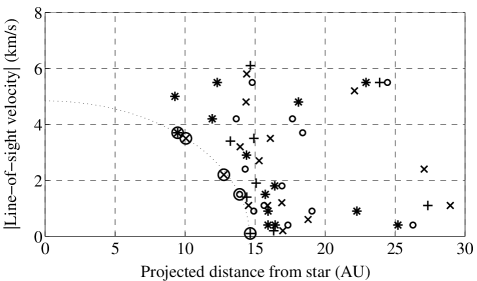
Figure 5: The absolute value of the line-of-sight velocity relative to that of the star (1 km s^-1) plotted against the projected distance of all the spatial components listed in Table 3 from the origin (the central star). The epochs are represented by the same symbols as in Fig. 4. Five of the components (marked by surrounding circles) fit accurately to an ellipse (dotted line) centred on the origin and with its axes along the coordinate axes of the diagram. If the expansion of the stellar envelope is isotropic, this suggests that there exists an inner distance (14 – 16 AU) at a certain expansion velociy (4 – 6 km s^-1) where water vapour masers first appear in the expanding gas.

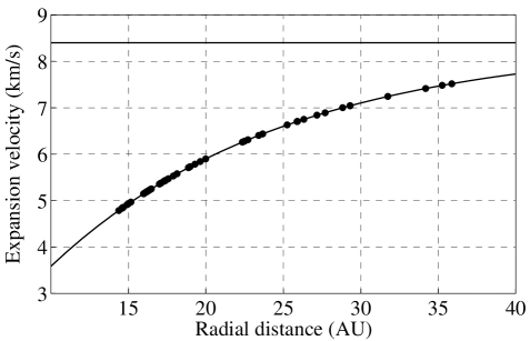
Figure 6: The model expansion velocity as a function of the distance from the star (Eq. 3). It approaches the terminal velocity (8.4 km s^-1) asymptotically (horizontal straight line). The dots along the expansion law curve symbolise the distances and velocities of the maser components.

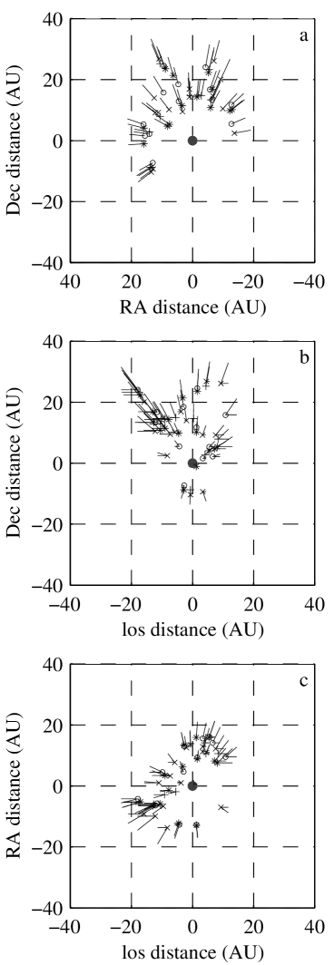
Figure 7: The three-dimensional distribution of maser components and their associated velocities according to the expansion model given by Eq. (3). The distribution is seen from three cardinal directions: on the sky (a), ‘from the side’ (b) and ‘from above’ (c). The maser components are represented by the same symbols as earlier. In addition the projected expansion velocities and the line-of-sight velocities are shown in the same scale in units of km s^-1 as the distance scale in units of AU.

5.2 The 3-D structure

By assuming a plausible expansion law it is possible to get a rough idea of the three-dimensional structure of the envelope. Supported by theoretical models of radiation-pressure-driven mass loss from late-type stars (cf. Goldreich & Scoville Goldreich76 (1976) and Bowen Bowen88 (1988)) we assume that the expansion law is exponential in nature and leading asymptotically to the final velocity, $v_{\rm f}$:

$$v=v_{\rm f}\left\{1-{\rm exp}\,\left[-k(r-r_{0})\right]\right\}$$ (3)

where $k$ is a scaling factor and $r_{0}$ is a radial shift.

Eq. (3) thus contains three constant parameters ($v_{\rm f}$, $k$ and $r_{0}$) and in order to find plausible values for them we need to estimate the coordinate values for three points on the expansion law. The value of $v_{\rm f}$ (the expansion velocity at $r=\infty$) can be estimated from (sub)-millimetre CO data, because it is believed that CO emission originates from gas throughout the CSE to very large distances from the star. We have two estimates of the terminal expansion velocity available: 9.3 km s^-1 (Olofsson et al. Olofsson02 (2002)) and 7.5 km s^-1 (Teyssier et al. Teyssier06 (2006)). Both these values are the results of complicated model fits involving several rotational CO lines. Therefore we are unable to judge the correctness of these results and we simply assume that they reflect the uncertainty inherent in the two models that give rise to them. Therefore we adopt the mean value of 8.4 km s^-1 for the value of the final expansion velocity.

In addition, we have a rough idea of the expansion velocity at one distance from the star (4.8 km s^-1 at 14.6 AU) from the analysis of the diagram in Fig. 5.

Finally, we assume that the expansion law is purely exponential all the way down to the photosphere, which is stationary, and where the expansion velocity is zero.

Thus the values of the parameters $k$ and $r_{0}$ can be determined from the condition that the stellar wind passes the positions $(r_{1},v_{1})=(14.6,4.8)$ and $(r_{2},v_{2})=(1.5,0)$:

$$k=\frac{{\rm ln}\,v_{\rm f}-{\rm ln}\,(v_{\rm f}-v_{1})}{r_{1}-r_{0}}$$ (4)

and

$$r_{0}=r_{2}=r_{*}$$ (5)

resulting in $k=0.065\,{\rm AU}^{-1}$ and $r_{0}=1.5\,{\rm AU}$.

Now, the observables are the line-of-sight velocity relative to the star $(v_{\rm los}-v_{*})$ and the projected radial distance $r_{\rm p}$. Their relations to the physical expansion velocity $v$ and radial distance $r$ are:

$$v_{\rm los}-v_{*}=v\,{\rm sin}\,\theta$$ (6)

and

$$r_{\rm p}=r\,{\rm cos}\,\theta$$ (7)

where $\theta$ is the angle between the normal to the line of sight and the radius from the star to the maser. Therefore, for every maser component the angle $\theta$ can be determined from the equations (3), (6) and (7).

In Fig. 6 the expansion law is shown graphically together with the maser component values determined by the model and represented by filled circles. They are shown mainly as an indication of the distance range for the maser components ($\sim$14 to $\sim$36 AU).

The 3D-distribution of the maser components and their associated velocities is shown in Fig. 7 as seen from three different directions: on the sky (a; similar to Fig. 4 but with the projected expansion velocities added), ‘from the side’ (b) and ‘from above’ (c). The dominance of tangential masers is seen clearly in Fig. 7 (b) and (c). The obliquity of the ‘maser arc’ seen in Fig. 7 (c) is in accordance with the preference of negative line-of-sight velocities on the lower-RA side of the star and of positive line-of-sight velocities on the higher-RA side, which is evident in Fig. 4.

However, one should keep in mind that an observer seeing RX Boo from directions deviating considerably from the geocentric direction would see a different set of maser components. Thus, Fig. 7 is merely showing the three-dimensional positions of the maser components that we see from earth. Most of them probably would be too weak to be detected from the directions represented by Figs. 7 (b) and (c). Of course a similar situation prevails for our present point of observation: there may be maser spots that we do not see because their emission may happen to be beamed in the wrong direction from our vantage point.

Having adopted an expansion law it is of interest to investigate the associated time scale for the gas to travel through the envelope. Thus, we have integrated the function $1/v$, where $v$ is described by Eq. (3), along the radius $r$, avoiding $r=r_{0}=1.5$ AU where $v=0$. We find that it takes $\sim$16.5 years for gas to travel through the zone (14 – 36 AU) where the H₂O masers reside.

6 Single dish data of SV Peg

The SRV SV Peg was selected for monitoring because of the detection of several maser features in 1990 not seen in previous spectra. We suspected that this star may show different variability properties compared to RX Boo. The H₂O maser was detected for the first time in 1974 by Dickinson (Dickinson76 (1976)), showing a strong line of $\sim$60 Jy at a line-of-sight velocity of 2 km s^-1. The maser was re-detected by Engels et al. (Engels88 (1988)) in 1984 showing two lines at 2 and 9 km s^-1 with similar flux densities of $\sim$12 Jy. The development of the maser emission since 1990 is shown in Fig. 8. The maser was observed also by Benson & Little-Marenin (Benson96 (1996)) in 1990 and by Takaba et al. (Takaba94 (1994)) in 1991 yielding line profiles that were similar to ours.

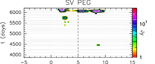
Figure 8: Flux density of the H₂O maser of SV Peg as a function of velocity and time. The time axis covers the years 1990 – 1995 (bottom) and 2000 – 2007 (top). The time stamp $t=0$ corresponds to 1990 February 17 (J.D. 2447933). The dotted horizontal lines mark the actual observations averaged in 4-day intervals. Flux densities in between the observations were interpolated linearly. The dashed vertical line marks the stellar systemic velocity (5 km s^-1) as given by Kerschbaum & Olofsson (Kerschbaum99 (1999)). The spectra were resampled to a resolution of 0.3 km s^-1. Contours in the lower panel are drawn at levels 3.00, 4.19, 5.86, 8.18, 11.43, 15.97 Jy (logarithmic scale) and in the upper panel at 3.00, 4.40, 6.45, 9.45, 13.86, 20.32 Jy. These levels are indicated by black and white lines in the flux scales along the right side of the two maps. (For a colour version of this figure, see the electronic edition.)

Our monitoring of SV Peg covered two periods 1990 – 1995 and 2000 – 2007. Sample spectra are shown in Fig. 9. Until 1992 the integrated maser emission was dominated by different single maser features with flux densities $>$10 Jy. Such features were not observed after 1992 and the integrated maser emission correspondingly declined abruptly during the first period. Also after the monitoring restart in the year 2000 the maser emission remained weak or absent until mid 2006. All spectra taken are shown in the Appendix (Figs. 19 – 22).

The H₂O masers of SV Peg appeared non-simultaneously over a velocity interval of 0 to 16 km s^-1. Actually, maser emission in the outer parts of this interval ($v_{\rm los}<2$ and $>$10 km s^-1) was detected only during 1990 – 1993. The velocity range of the maser in general would be severely underestimated, if its determination were based on individual spectra alone.

Compared to RX Boo the spectral profiles of SV Peg are different. While for RX Boo generally maser emission was detected over the full velocity range and the individual features are strongly blended, the SV Peg maser features are usually well separated. This is in part due to the weakness of the SV Peg features, of which mostly only the brightest were detected. But even during the bright phases around 1991 and near the end of 2006 most features are well separated suggesting that the number of individual maser features is lower in SV Peg compared to RX Boo.

Figure 9: Sample H₂O maser spectra of SV Peg showing typical profiles starting in 1990 and ending in early 2007. Note the varying flux density scale.

Like we did for RX Boo (cf. Sect. 3.3) we made a line profile analysis for SV Peg by fitting multiple Gaussian components to the maser profiles. As before, we assumed that maser features in adjacent spectra with velocity differences $\la$0.5 km s^-1 belong to a unique physical maser component in the shell of SV Peg. All features were assigned to 9 maser spectral components labelled A, B,…, H. These components are listed in Tables A and A in the Appendix. For a description of the tables we refer to Sect. 3.3.

Except for features B and C we find that all spectral components are fairly well separated in velocity. Therefore the central velocities show in general a small scatter ($\la$0.5 km s^-1). Larger drifts in velocity ($\la$1.5 km s^-1) are seen in component B indicating the presence of blends. Almost all features dominated the spectral profile at some epochs. The typical timescales for major intensity variations of individual components were 6 – 12 months. A particularly well defined example for the temporary appearance of a feature is component F ($v=11.3$ km s^-1 in Fig. 8; Fig. 9, Date: 1991 March 30), which was detected for 11 months only. Noticeable is also the spectral feature H at +16.4 km s^-1, which was observed only twice in the beginning of 1992 (cf. Fig 9, Date: 1992 February 29). We consider this feature as real, although it was detected at the $2-3\sigma$ level only.

Summarizing, the case of SV Peg shows that the H₂O maser is composed of at least 8 components, where each of them dominated the profile for several months. At any given epoch, maser emission was only seen for a limited fraction (a few km s^-1) of the whole velocity span liable to exhibit a maser. Thus the non-detection of H₂O masers in many SRVs might be merely a temporary effect, and the detection rate of 20% obtained by Szymczak & Engels (Szymczak95 (1995)) among SRVs using two observing epochs separated by four months might be raised considerably with observations separated by years.

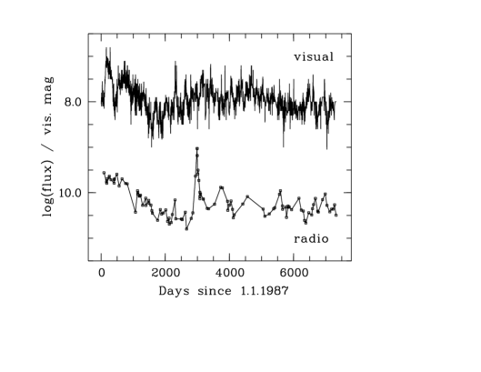
Figure 10: Optical AAVSO lightcurve and the lightcurve of the integrated H₂O maser emission for RX Boo during the years 1987 – 2007. The optical data are visual magnitudes and the integrated radio flux has been offset by an arbitrary amount.

7 Radio and optical variability in SRVs

It has been reported that the variability of the H₂O maser emission of RX Boo is weakly correlated with the optical lightcurve, and that different maser features react to optical variations with different time delays (Hedden et al. Hedden91 (1991)). The optical and the radio lightcurve during the period 1987 – 2007 is shown in Fig. 10. The optical data given as visual magnitudes were obtained from the American Association of Variable Star Observers (AAVSO; Hedden Hedden07 (2007)). We rebinned the data into three-day intervals and interpolated over intervals without observations. The integrated radio fluxes were taken from Table A in the Appendix.

A cross correlation between the optical and the radio lightcurves has been performed with delays of up to 2000 days ($\sim$6 years) following the suggestion of Lekht et al. (Lekht05 (2001)) that the maser emission may respond to the passage of shock waves formed during a previous bright phase of the star. No significant signal has been found for any delay. However, the course of the lightcurves in Fig. 10 gives the impression that a weak correlation without significant delay is present with a timescale of several years. In particular, both lightcurves show a minimum at 2000 days (1992 – 1993).

We searched also for particularly bright phases in the optical lightcurve before 1995, which could have caused the strong radio flare in 1995 March ($t\approx 3000$). Such optically bright phases occurred irregularly every few years, while the strength of the flare was unique during our observing period. It was therefore not possible to link the radio flare with a particular part of the optical lightcurve.

We made a similar analysis of the correlation between optical and maser variations for SV Peg with negative result. Lekht et al. (Lekht99 (1999)) observed the maser variations of another SRV RT Vir over the period 1985 – 1998 and found large amplitude variations including two flares with flux densities $>$1000 Jy. Although they do not discuss the optical behaviour of the star during this time, available AAVSO optical data do not show any magnitude variations larger than the usual $\pm 0.5$ mag around the mean $m_{\rm vis}\approx 8.9$. We conclude therefore that there is basically no correlation between H₂O maser radio data and optical data for SRVs.

8 Discussion

The long-term monitoring programme of the two SRVs RX Boo and SV Peg allows us to draw a few general conclusions on the variability properties of their H₂O masers.

• Maser emission occurs over a fixed velocity range $\Delta v$, but not necessarily at all velocities simultaneously. There is no evidence that the velocity range varied systematically with time. Occasionally, maser emission outside the regular velocity interval may appear.

• The individual maser features vary irregularly and any correlation with the optical variability of the stars is negligible compared to these irregular variations. The intensity of a particular feature characterises this feature alone and is not representative for the maser emission as a whole. The integrated intensity obtained over the velocity range $\Delta v$ is a more suitable measure to describe the maser “activity” at a given epoch.

• The lifetime of individual maser components is of the order 1 year, much less (5 – 10%) than the time needed for a mass element to cross the H₂O maser shell.

• The distribution of the maser spatial components in the circumstellar shell of RX Boo has been found to be remarkably stable over the range of 6 years (1990 – 1995). The distribution showed a persistent asymmetry, with emission coming always from the NE part and never from the SW part of the shell. The likelihood to find a new maser component in the shell, is higher in those parts, where a maser has been observed previously.

8.1 RX Boo velocity range

During the monitor programme the H₂O maser velocity range of RX Boo never exceeded the interval $-5\la v_{\rm los}\la+5$ km s^-1 (Fig. 2). This is well within the velocity range defined by CO emission extending from –8.3 to +10.3 km s^-1 according to Olofsson et al. (Olofsson02 (2002)) or –6.5 to +8.5 km s^-1 according to Teyssier et al. (Teyssier06 (2006)), although the H₂O interval is not symmetric with respect to the stellar velocity of $v_{*}=+1$ km s^-1 as defined by the CO lines (see also Sect. 8.7). Larger velocity ranges have been observed in the past (Engels et al. Engels93 (1993)). Before 1983 the strongest feature was always detected at $v_{\rm los}\approx 6$ km s^-1 (see the compilation in Engels et al. Engels88 (1988)), which is well beyond the red edge of the current velocity interval. On one occasion, in 1982.2, emission was detected even over an interval $-11<v_{\rm los}<+9$ km s^-1 (Johnston et al. Johnston85 (1985); de Vegt et al. deVegt87 (1987)), almost twice the range observed in 1980 (Dickinson & Dinger Dickinson82 (1982)) and after 1990.

Except for this one occasion, the larger maser velocity range can be explained within our model (cf. Sect. 5), as line-of-sight velocities $|v_{\rm los}-v_{*}|$ up to the adopted final outflow velocity $v_{\rm f}=8.4$ km s^-1 are permitted. According to Eq. (6) a larger $|v_{\rm los}-v_{*}|$ would require a larger outflow velocity $v$ at the maser site and/or a larger $\theta$. Following Eq. (7) the latter implies a smaller projected distance $r_{\rm p}$ of the maser site. Because the outflow velocity increases outwards, larger $|v_{\rm los}-v_{*}|$ are achieved at larger radial distances from the star and RX Boo may have at some time sustained H₂O maser emission in the outer reaches of the shell. On the other hand, in the case of a smaller $r_{\rm p}$, maser components may have been present within the inner projected ring drawn in Fig. 4, in which no emission was detected after 1983.

Maser emission at larger radial distances might have been possible due to a temporal increase in luminosity of the star allowing the rise of the temperature in the shell or due to the passage of a subshell with increased density. In the former case the minimum temperature required to excite H₂O masers will be achieved at larger radii than normally. However, the mean optical brightness of the star was not brighter before 1983 than afterwards, making this explanation unlikely. In the latter case the size of the shell having the minimum density required to excite H₂O masers might have been increased for some time.

On the other hand, maser sites with smaller $r_{\rm p}$ could have been triggered by local enhancements of the gas density or by temporary increases of gain lengths. Such sites could be located at any distance from the star, but we would be seeing a maser that has become more ’radial’. All these possible causes can be probed during future periods, if RX Boo should again display an extended velocity range, by searching for an increase of the outer shell radius, or by searching for maser components within the inner ring.

At odds with our hypothesis is the 1982.2 observation, where the blueshifted emission exceeded the blue edge of the CO velocity range by 3 – 4 km s^-1. This observation apparently has recorded a faster than usual outflow, crossing the H₂O maser shell by 1982.

8.2 SV Peg velocity range

The observed velocity interval in SV Peg is 0 to +16.5 km s^-1. This is to be compared to the CO emission velocity interval –2.5 to +12.5 km s^-1 (Olofsson et al. Olofsson02 (2002)), which implies a stellar radial velocity $v_{*}=+5$ km s^-1 and a final outflow velocity of 7.5 km s^-1. H₂O maser emission at the most blue-shifted velocities $v_{\rm los}<0$ km s^-1 was never observed, while emission at the redshifted final outflow velocity was seen in 1990 – 1992 (spectral components F and G). This implies that the final outflow velocity is already reached within the H₂O maser shell.

As in the case of RX Boo before, also SV Peg showed emission outside the CO velocity range. Spectral feature H at +16.4 km s^-1 (outflow velocity 11.4 km s^-1), which was seen only in 1992, might have traced an outflowing mass segment with temporarily higher speed than is normally achieved in the CSE of SV Peg.

8.3 H₂O maser shell size of RX Boo

Unless there are 100% tangentially beaming maser clouds at the outer periphery of the shell, the observed diameter $\phi_{\rm p}$ of the H₂O maser shell will be smaller than the true diameter $\phi$ because of projection effects. As the most distant maser regions are usually weak, the observed diameter is certainly depending also on the sensitivity of the observations. Finally the diameter will depend on the assumptions made with respect to the location of the star relative to the observed distribution of maser clouds.

For 1982 Johnston et al. (Johnston85 (1985)) give a projected diameter $\phi_{\rm p}=200$ mas compared to $\phi_{\rm p}=140$ mas in 1983 (Lane et al. Lane87 (1987)) and $\phi_{\rm p}=150$ mas in 1985 (Bowers et al. Bowers93 (1993)). This apparently confirms the case, that the large velocity range in 1982 was due (at least in part) to a more extended H₂O maser shell. However, Colomer et al. (Colomer00 (2000)) determined $\phi_{\rm p}=230$ mas for 1990 June and we fitted $\phi_{\rm p}=180$ mas for the bulk of the emission features observed in 1990 – 1992, however, omitting outlying components at radial distances $100<r_{\rm p}<160$ mas for the adopted stellar position. Usually the stellar position is adopted in the centre of the maser spot distribution, which leads to the smallest projected diameters possible. Our proposal for the position of the star relative to the masers is offset by $\sim$50 mas from the centroid of the maser emission, which leads to an unprecedented high $\phi_{\rm p}=320$ mas. Thus the implied projected shell diameter is 51 AU. According to our model the component with the highest radial distance from the star has $r\sim 36$ AU, which implies that the true angular diameter of the shell might be as high as $\phi=440$ mas. So far, a variation of the H₂O maser shell size of RX Boo cannot be determined, because the differences in the diameters derived by different authors are still dominated by data quality and model assumptions.

8.4 The connection of maser variations with stellar variations

Long-term monitoring of H₂O maser emission has been made by Lekht et al. (Lekht05 (2001) and references therein) for various SRVs, Mira variables, and RSGs. For the objects with large-amplitude variations they find that the integrated H₂O maser emission is correlated with the optical emission of the star. The radio emission lags behind the optical one by a few tenths of the period. They generally favour a model, in which the variations of the H₂O masers are due to passages of shock waves generated on the stellar surface. The long travelling times ($>$10 years), however, make it difficult to find correlations between the optical and radio lightcurves over such delays.

However, the luminosity variations of the star certainly affect the excitation conditions in the whole maser shell. The response of H₂O masers to the light variations in general is well documented for Mira variables (e.g. Lekht et al. Lekht01 (2001); Brand et al. Brand02 (2002)) and OH/IR stars (Engels et al. Engels86 (1986)). For the SRVs studied here the variations of the integrated radio flux are largely caused by brightness variations of single maser features, and not by variations at all velocities simultaneously. We argue therefore that the H₂O maser variations in SRVs are dominated by local effects, such as variations of the velocity coherence length due to turbulence. The influence of the stellar luminosity variations on the maser variation is negligible in these stars.

8.5 The lifetime of individual maser clouds

The changes seen in the VLA maps as well as the velocity shifts seen over time for spectral components determine a typical lifetime of maser clouds in the range 0.5 – 3 years (Sect. 4.5). This is in excellent agreement with the estimates derived from H₂O maser cloud imaging of four AGB stars of Bains et al. (Bains03 (2003)), who argue that instability will destroy the clouds on such time scales. They derived sound crossing times of 1.5 – 3 years for the observed sizes of the clouds.

Based on observations with the VLBA Imai et al. (Imai03 (2003)) derived for RT Vir clouds considerably shorter lifetimes of 1 – 2 months. This order of magnitude shorter lifetime compared to ours is probably due to different spatial resolutions. The number of clouds identified in a particular maser shell is significantly increased when the spatial resolution is increased. For example, Marvel (Marvel96 (1996)) distinguished $>$50 maser clouds in VLBA RX Boo H₂O maser maps, while we were restricted to $<$15. Thus, the clouds identified here for RX Boo are certainly composed of several sub-components, where each of them might survive on the timescale of months only. Our larger lifetimes apply then to spatially closely located groups of maser clouds (our maser spatial components), of which the spectral components in single-dish spectra are made. The dependence of the lifetimes on the size of the maser clouds is also evident from observations of RSGs, where the clouds have physical diameters a magnitude larger than are observed in AGB stars, and lifetimes of the order of 10 years (Richards et al. Richards98 (1998) and Richards99 (1999)).

The typical gas crossing time through the H₂O maser supporting shell in RX Boo (thickness $\sim$22 AU) is $\sim$16.5 years (Sect. 5). The maser clouds most probably do not survive a full crossing of this shell. Due to the limited lifetimes of the maser clouds proper motion measurements require therefore an observing frequency high enough to sample a given cloud at least twice. At the highest resolutions achievable today, recurrent observations with intervals less than a month are reasonable (see Imai et al. Imai03 (2003)).

8.6 The beaming directions of masers in the RX Boo shell

The distribution of maser components in Fig. 4 tells us that the individual masers are radiating non-isotropically in the sense that their maximum output is in a direction that does not deviate very much from the tangential direction. Our model of the shell expansion has given us values of the angle $\theta$ (the aspect angle) for every maser component. The distribution function of these values has a maximum at zero degrees and an extent from about –60° to +60°. In other words, the masers are not all in a plane perpendicular to the line of sight [see Figs. 7(b) and (c))].

Now, imagine for a moment that all masers were radiating in the tangential direction and that we therefore see many of them from an angle that deviates from the direction of maximum amplification. Furthermore, assume that all the masers have the same intrinsic strength. Then by plotting the observed flux density against the aspect angle we would get the ‘beam shape’ of the ‘unit maser’. Of course there is probably a spread in the direction of maximum amplification from the tangential direction. Also there is certainly a considerable spread in the intrinsic strength of the masers. These spreads would destroy to a large extent the relation between flux density and aspect angle. However, it is conceivable that a weak correlation would remain.

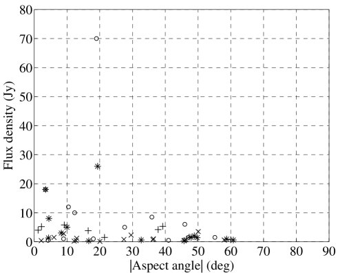
Figure 11: The observed flux density as a function of the absolute value of the aspect angle ($\theta$). The epochs are represented by the same symbols as in Figs. 4 and 5.

In Fig. 11 the observed flux density is plotted against the absolute value of the aspect angle. It is obvious that the highest fluxes are found among the smallest aspect angles. If the two data points with the very high fluxes close to 20° are disregarded the highest flux indeed is found close to 0°. In addition, the upper envelope of the scatter plot is decreasing from a maximum close to 0° to a minimum close to 60°. The fact that this correlation is disturbed by the very strong masers at 20° must be explained by the disparate intrinsic maser strengths.

Fig. 11 is an additional evidence, albeit a weak one, for the H₂O masers in the CSE of RX Boo to be predominantly tangentially beamed. However, the typical beaming angle is impossible to extract from the data as we cannot disentangle the deviation of the line of sight from the direction of the maximum amplification and the deviation of the direction of the maximum amplification from the tangential direction.

8.7 Maser shell asymmetry

So far, the H₂O maser shell has been assumed to be radially symmetric. However, there is a prominent asymmetry present in the distribution of H₂O maser emission of RX Boo, which manifests itself during 1990 – 1995 by the absence of emission in the SW part of the shell and by the NW-SE velocity gradient (Sect. 4.4). How persistent is this asymmetry? Interferometric observations of the H₂O masers of RX Boo have been made a number of times, but the first sensitive map available is from VLA observations in 1985 (Bowers et al. Bowers93 (1993)). An E-W velocity gradient is evident also in this map, but in addition there is some emission in the SW part of the shell. VLBA observations taken in 1995 January and July are available from Marvel (Marvel96 (1996)), but they are difficult to compare with our VLA maps because all the blueshifted emission with $v_{\rm los}<+0.5$ km s^-1 was not detected. This emission seems to have been resolved out. Nevertheless, we conclude that the incomplete ring-like structure and the velocity gradient was present at least over eleven years between 1985 and 1995, which is about 70% of the gas crossing time in the H₂O maser-supporting shell of RX Boo.

Evidence for asymmetry is coming also from the H₂O-maser velocity interval, which is centred on $v_{\rm c}=0$ km s^-1 (Fig. 2), while the CO-emission velocity interval is centred on $v_{*}=+1$ km s^-1 (Teyssier et al. Teyssier06 (2006)). The blueshifted projected expansion velocities extend to higher values $|v_{\rm los}-v_{*}|\,\approx 6$ km s^-1 than the redshifted velocities $|v_{\rm los}-v_{*}|\,\approx 4$ km s^-1. This velocity asymmetry has persisted over the full monitoring time range of 20 years.

Figure 12: Upper envelope of all spectral profiles of RX Boo (top) and SV Peg (bottom). In RX Boo the spectra containing the flare (1995 January – May) were omitted. The flare occured at $\sim$3.5 km s^-1 close to the strongest peak in the upper envelope and reached a peak flux of 1600 Jy. The upper envelope is defined as the highest flux density ever achieved in velocity bins of 0.3 km s^-1 during the monitoring program.

In Fig. 12 the upper envelopes of the spectral profiles of RX Boo and SV Peg are shown. These envelopes show the highest flux densities measured during the monitoring period at each velocity. Contrary to SV Peg, where the highest flux densities are more or less on a similar level across the maser velocity range, the profile of RX Boo is dominated by emission at $\sim$2.5 km s^-1 (spectral component I). Emission close to this velocity was present over the full monitoring period (see Table A in the Appendix), emphasizing the longevity of the asymmetries.

Asymmetries present in individual observations can easily be explained as due to shells unevenly filled with maser clouds. The clouds themselves are explained by Richards et al. (Richards99 (1999)) as clumps of enhanced density, which form as condensations in the extended stellar atmosphere. Due to the randomness of the formation process of such clumps, parts of the shell might not contain clumps at a given epoch. But we have observed the persistence of the asymmetric emission structure and the velocity gradient over a time range more than half of the crossing time through the shell. And, the asymmetry of the H₂O maser velocity interval outlasted the 16.5 years crossing time, showing that the morphology of the maser site distribution is not due to random fluctuations. It is therefore more likely that the persistent asymmetries are evidence for a non spherically-symmetric mass loss process in RX Boo. The asymmetric distribution of maser emission components found in RX Boo is not untypical. ¿From VLA-observations of H₂O masers in 13 Mira variables and 3 SRVs, Bowers & Johnston (Bowers94 (1994)) concluded that the emission is best modelled by “clumps, segments, or filaments in an asymmetric but ellipsoidal-type geometry”.

For a strong maser to occur, some very special (and rare) physical conditions have to be fulfilled: the pumping of the masing transition has to win over thermal de-excitation processes and the coherent amplification path length has to be sufficiently long for the maser flux density to be detected. Therefore, an alternative explanation of the asymmetric distribution of H₂O masers in the envelope of RX Boo might be provided by a non-spherical distribution of maser conditions.

A possible explanation of such a distribution might be found in the photospheric structure of the star. Giant and supergiant stars have extremely deep convective layers and as a result the convection cells of the photosphere are expected to be gigantic (cf. Schwarzschild Schwarzschild75 (1975)). Freytag (Freytag03 (2003)) has made a 3-dimensional radiative hydrodynamic model of the SRV Betelgeuse ($\alpha$ Orionis; spectral class M2Iab) that simulates high-resolution observations of surface features (cf. Young et al. Young00 (2000)) and typical irregular flux variations of this star (cf. Goldberg Goldberg84 (1984)). However, we are unaware of any published simulations of pulsating giants or of AGB stars of more moderate sizes. Nevertheless, it is conceivable that the random character of the convection elements is responsible for irregular light variations or for an irregular modulation of periodic variations. It is conceivable too that the convection elements to a certain degree are preserved as some kind of ‘blobs’ in the stellar wind. As these blobs reach the H₂O maser region, a larger blob probably creates longer amplification path lengths than a number of smaller blobs. In addition such blobs will expand considerably during their travel outwards, not only due to the divergence but also radially due to the acceleration. In the case of RX Boo a convective blob is expected to increase its volume by a factor of $\sim$50 during its journey from the photosphere to the inner radius of the H₂O maser region.

However, the real mystery is the longevity of the asymmetry of the H₂O maser region of RX Boo. In the convection-wind picture this implies that the lifetime of convection cells either be long or that the occurence of large cells persists over long time periods. In the Betelgeuse simulation by Freytag (Freytag03 (2003)) the lifetime of convection cells seems to be of the order of one year and the likelihood of occurence of a cell seems to be constant over both time and stellar surface. If the typical lifetime of convection cells in the RX Boo photosphere is of the same order, it would take about one year for the corresponding blob to getting detached from the photosphere and becoming part of the stellar wind. However, when this blob reaches the H₂O maser region ($\sim$14 AU from the star), the inflation due to acceleration and divergence would increase the time for the blob to pass a fixed point by a factor of about 5.

9 Conclusions

Water vapour maser emission from CSEs is often strong enough to be observed with small radio telescopes even in rather distant late-type stars. Because of its variability, however, the information to be derived from a single maser spectrum is limited. Neither the intensities nor the velocities are necessarily representative. To understand the cause of the strong variability of the masers in SRVs we have monitored RX Boo and SV Peg, two stars representative of their class, with single-dish radio telescopes over a period of two decades. The interpretation of the variations seen in single-dish spectra is usually compromised by blending of the maser peaks due to the overlap of two or more maser clouds in velocity space. To overcome this limitation, we obtained in addition for RX Boo four interferometric observations taken over a time interval of almost three years.

We find that the H₂O masers in RX Boo are located in an incomplete ring of thickness 22 AU, which is filled only in part. The time that the gas needs to cross this ring is 16.5 years. This ring-like distribution of maser spots remained stable over at least 11 years. Compared to these timescales, the survival time of individual maser clouds is much shorter having a typical duration of $\sim$1 year. The variability of H₂O masers is then due to the emergence and disappearance of shortlived maser clouds. The variations in intensities of these clouds are not dependent on variations of the stellar luminosity, as we find no correlation between the optical and the radio lightcurve.

It follows from the interpretation of single-dish spectra that the strength of individual maser peaks or the details in the shape of the profile are snap-shots reflecting the distribution of the maser clouds and their luminosities at the time of observation. If RX Boo and SV Peg are typical SRVs, the lifetime of these clouds in SRVs is limited to about 1 year. Also stellar radial velocities and shell outflow velocities will be biased, if the maser cloud distribution is not uniform in the shell.

For RX Boo, the persistent overall distribution of the maser emission regions indicates that the underlying mass outflow from the star or the distribution of maser conditions are not spherically symmetric. Whether deviations from spherical symmetry are present in the H₂O maser regions of SRVs in general, will have to be answered by new monitoring programmes relying on interferometry for a larger sample of stars.

Appendix A Single-dish data of RX Boo and SV Peg

[x]rrcrrr—rr—rr—rr—rr

Maser components of RX Boo. The columns give the observing date in Gregorian and Julian (JD) format, the noise of the spectra (rms), the integrated flux $S_{\rm{I}}$ in units of $10^{-22}$ W m^-2, and the velocities $v_{\rm{p}}$ and flux densities $S_{\rm{p}}$ of maser peaks associated with the spectral components A – E in Table 3.

A B C D E

Date JD rms $S_{\rm{I}}$ $v_{\rm{p}}$     $S_{\rm{p}}$ $v_{\rm{p}}$     $S_{\rm{p}}$ $v_{\rm{p}}$     $S_{\rm{p}}$ $v_{\rm{p}}$     $S_{\rm{p}}$ $v_{\rm{p}}$     $S_{\rm{p}}$

[Jy]  [km s^-1, Jy]

continued.

A B C D E

Date JD rms $S_{\rm{I}}$ $v_{\rm{p}}$     $S_{\rm{p}}$ $v_{\rm{p}}$     $S_{\rm{p}}$ $v_{\rm{p}}$     $S_{\rm{p}}$ $v_{\rm{p}}$     $S_{\rm{p}}$ $v_{\rm{p}}$     $S_{\rm{p}}$

[Jy]  [km s^-1, Jy]

30.03.87 2446885 3.41 2743 $-$ $-$ $-$ $-$ $-$ $-$ $-$ $-$ $-$ $-$
22.06.87 2446969 1.16 1732 ———————       $-3.8$     4:       ———————   $-$ $-$
05.09.87 2447044 2.30 2170 $-$ $-$ $-$ $-$ $-$ $-$ $-$ $-$ $-$ $-$
12.09.87 2447051 4.41 2305 $-$ $-$ $-$ $-$ $-$ $-$ $-$ $-$ $-$ $-$
05.11.87 2447105 5.16 1928 $-$ $-$ $-$ $-$ $-$ $-$ $-$ $-$ $-$ $-$
11.02.88 2447203 0.86 1927 $-$ $-$ $-$ $-$ $-$ $-$ $-$ $-$ $-$ $-$
19.02.88 2447211 4.27 2018 $-$ $-$ $-$ $-$ $-$ $-$ $-$ $-$ $-$ $-$
02.05.88 2447284 5.55 2544 $-$ $-$ $-$ $-$ $-$ $-$ $-$ $-$ $-$ $-$
13.07.88 2447356 2.56 1410 ———————       $-3.6$     14:       ———————   $-$ $-$
13.10.88 2447448 4.06 2009 ———       $-4.2$     18.5       ———   $-2.4$ 23.1 $-$ $-$
31.01.89 2447558 2.53 1599 ———       $-3.9$     16:       ———   $-2.4$ 42.7 $-$ $-$
21.03.89 2447607 3.79 1571 $-$ $-$ $-$ $-$ $-$ $-$ $-2.4$ 32.5 $-$ $-$
04.12.89 2447865 1.44 374 $-$ $-$ $-$ $-$ $-$ $-$ $-$ $-$ $-$ $-$
06.02.90 2447929 0.95 1105 $-4.8$ 2.8 $-$ $-$ $-3.0$ 6.0 $-$ $-$ $-$ $-$
17.02.90 2447940 0.25 1008 $-4.6$ 2.6 $-$ $-$ $-2.9$ 6.2 $-$ $-$ $-$ $-$
31.03.90 2447982 0.14 842 $-4.7$ 3.9 $-$ $-$ $-2.9$ 5.7 $-$ $-$ $-1.3$ 1.6
17.04.90 2447999 0.95 845 $-$ $-$ $-$ $-$ $-$ $-$ $-$ $-$ $-$ $-$
11.05.90 2448023 0.22 883 $-4.6$ 4.9 $-$ $-$ $-2.9$ 4.5 $-$ $-$ $-1.2$ 1.7
15.07.90 2448088 1.84 528 $-$ $-$ $-$ $-$ $-3.0$ 3.0 $-$ $-$ $-$ $-$
21.10.90 2448186 0.13 759 $-4.5$ 5.0 $-$ $-$ $-2.5$ 4.4 $-$ $-$ $-1.2$ 1.3
18.01.91 2448275 1.94 680 $-$ $-$ $-$ $-$ $-2.7$ 8.5 $-$ $-$ $-$ $-$
29.01.91 2448286 1.82 587 $-4.7$ 6.4 $-$ $-$ $-2.9$ 5.4 $-$ $-$ $-$ $-$
30.03.91 2448346 0.10 534 $-4.6$ 3.4 $-$ $-$ $-2.6$ 3.5 $-$ $-$ $-$ $-$
01.05.91 2448378 0.26 404 $-4.6$ 3.0 $-$ $-$ $-2.7$ 4.7 $-$ $-$ $-1.0$ 0.8
17.05.91 2448394 1.33 354 $-$ $-$ $-$ $-$ $-2.9$ 9.2 $-$ $-$ $-0.8$ 1.3
25.10.91 2448555 0.72 249 $-$ $-$ $-$ $-$ $-2.7$ 4: $-$ $-$ $-$ $-$
18.01.92 2448640 0.19 426 $-4.5$ 1.9 $-3.7$ 1.2 $-2.8$ 3.7 $-1.9$ 2.6 $-$ $-$
29.02.92 2448682 0.12 340 $-4.6$ 1.6 $-$ $-$ $-2.6$ 3.3 $-$ $-$ $-$ $-$
18.04.92 2448731 0.64 359 ———————       $-3.3$     4:       ———————   $-$ $-$
05.07.92 2448809 0.18 418 $-4.5$ 2.9 $-$ $-$ $-2.5$ 5.6 $-$ $-$ $-$ $-$
01.09.92 2448867 0.10 234 $-4.8$ 4.6 $-3.6$ 3.9 $-2.3$ 4.6 $-$ $-$ $-$ $-$
15.10.92 2448911 0.69 277 ———————       $-3.5$     4.7       ———————   $-$ $-$
24.10.92 2448920 0.69 205 $-$ $-$ $-$ $-$ $-$ $-$ $-$ $-$ $-$ $-$
22.12.92 2448979 0.13 221 $-4.9$ 2.4 $-3.7$ 5.0 $-$ $-$ $-2.0$ 2.5 $-1.0$ 1.2
26.01.93 2449014 0.48 331 $-4.9$ 4.2 $-3.6$ 7.5 $-$ $-$ $-2.3$ 4.5 $-1.2$ 1.0
21.04.93 2449099 0.14 694 $-4.6$ 11.0 $-3.5$ 6.2 $-2.8$ 10.8 $-2.0$ 7.3 $-1.0$ 2.9
13.05.93 2449121 0.58 268 $-4.5$ 4.8 $-$ $-$ $-2.9$ 7.0 $-$ $-$ $-$ $-$
03.11.93 2449295 0.54 264 ———————       $-3.6$     5.8       ———————   $-$ $-$
30.11.93 2449322 0.23 257 $-$ $-$ $-4.0$ 4.0 $-2.8$ 3.0 $-$ $-$ $-$ $-$
08.03.94 2449420 0.22 373 $-$ $-$ $-4.2$ 4.5 $-3.4$ 3.4 $-2.1$ 3.9 $-$ $-$
14.04.94 2449457 0.34 160 $-$ $-$ $-$ $-$ $-3.2$ 1.7 $-$ $-$ $-$ $-$
08.09.94 2449604 1.35 272 $-$ $-$ $-$ $-$ $-$ $-$ $-$ $-$ $-$ $-$
28.10.94 2449654 0.61 361 $-$ $-$ $-4.2$ 3.9 $-3.4$ 3.0 $-2.1$ 3.4 $-$ $-$
18.01.95 2449736 0.85 2319 $-$ $-$ $-$ $-$ $-$ $-$ $-$ $-$ $-$ $-$
09.03.95 2449786 0.47 9382 $-$ $-$ $-$ $-$ $-3.1$ 3.3 $-1.6$ 5.3 $-$ $-$
12.03.95 2449789 — 9408 $-$ $-$ $-$ $-$ $-$ $-$ $-$ $-$ $-$ $-$
13.03.95 2449790 0.33 6558 $-$ $-$ $-$ $-$ $-3.2$ 2.1 $-1.5$ 3.9 $-$ $-$
27.03.95 2449804 0.30 2585 $-$ $-$ $-$ $-$ $-$ $-$ $-$ $-$ $-$ $-$
09.04.95 2449817 0.20 3129 $-$ $-$ $-$ $-$ $-3$ $<$2 $-1.5$ $<$4 $-$ $-$
03.05.95 2449841 0.13 1869 $-$ $-$ $-$ $-$ $-3$ $<$2 $-1.5$ $<$5 $-$ $-$
03.06.95 2449872 0.21 1021 $-$ $-$ $-3.9$ 1.7 $-$ $-$ ——     $-1.0$     5.9     ——
04.06.95 2449873 0.23 739 $-$ $-$ $-3.8$ 1.2 $-$ $-$ ——     $-1.1$     4.2     ——
05.06.95 2449874 0.19 832 $-$ $-$ $-3.7$ 1.6 $-$ $-$ ——     $-1.2$     5.0     ——
23.06.95 2449892 0.22 947 $-$ $-$ $-$ $-$ $-3.2$ 2.7 $-$ $-$ $-1.0$ 9.1
18.09.95 2449982 0.19 728 $-$ $-$ $-$ $-$ $-$ $-$ $-2.1$ 10.0 $-$ $-$
18.01.96 2450101 0.08 453 $-$ $-$ $-$ $-$ $-2.6$ 1.8 $-$ $-$ $-0.9$ 2.9
01.03.96 2450144 0.93 447 $-$ $-$ $-$ $-$ $-$ $-$ $-$ $-$ $-0.9$ $<$5
03.09.96 2450330 0.17 560 $-$ $-$ $-$ $-$ $-2.8$ 2.6 ——     $-1.4$     2.2     ——
14.03.97 2450522 0.13 1316 $-$ $-$ $-$ $-$ $-2.7$ 10.7 $-$ $-$ $-$ $-$
06.05.97 2450575 0.71 1277 $-$ $-$ $-$ $-$ $-2.6$ 9.4 $-$ $-$ $-$ $-$
12.10.97 2450734 0.14 650 $-$ $-$ $-$ $-$ $-2.3$ 13.3 $-$ $-$ $-0.5$ 5.9
21.10.97 2450743 0.58 420 $-$ $-$ $-$ $-$ $-2.3$ 7.9 $-$ $-$ $-0.5$ $<$4
15.12.97 2450798 0.47 567 $-$ $-$ $-$ $-$ $-2.2$ 11.2 $-$ $-$ $-$ $-$
29.01.98 2450843 0.58 616 $-$ $-$ $-$ $-$ $-2.2$ 16.0 $-$ $-$ $-$ $-$
19.03.98 2450892 0.53 431 $-$ $-$ $-$ $-$ $-2.3$ 6.0 ——     $-1.2$     4.1     ——
10.04.98 2450914 0.80 281 $-$ $-$ $-$ $-$ $-$ $-$ ——     $-1.5$     $<$5     ——
11.05.98 2450945 0.74 327 $-$ $-$ $-$ $-$ ——     $-1.8$     5.3     ——   $-$ $-$
02.02.99 2451212 0.38 567 $-$ $-$ $-$ $-$ $-3.4$ 9.5 ——     $-1.2$     4.6     ——
24.06.99 2451354 0.12 824 $-$ $-$ $-$ $-$ $-3.6$ 31.7 ——     $-0.9$     $<$9     ——
27.10.00 2451845 1.00 437 $-4.4$ 9.9 $-$ $-$ $-$ $-$ $-$ $-$ $-0.6$ 16.4
20.12.00 2451899 0.79 304 $-4.2$ 3.3 $-$ $-$ $-$ $-$ $-$ $-$ $-0.6$ 7.2
07.05.01 2452037 0.65 343 $-4.3$ 2.2 $-$ $-$ $-$ $-$ $-$ $-$ $-0.9$ 4.8
18.09.01 2452171 0.66 442 $-$ $-$ $-$ $-$ $-$ $-$ $-$ $-$ $-1.0$ 14.5
24.10.01 2452207 0.76 469 $-$ $-$ $-$ $-$ $-$ $-$ $-$ $-$ $-1.0$ 12.6
19.03.02 2452353 1.89 922 $-$ $-$ $-$ $-$ $-$ $-$ $-$ $-$ $-$ $-$
18.04.02 2452383 0.80 1107 ———————-       $-6.0-0.0$     $\approx 2-4$       ———————-
20.06.02 2452446 0.15 512 $-$ $-$ ————–       $-4.0-0.0$     $\approx 2$       ————–
26.06.02 2452452 1.11 434 $-$ $-$ $-$ $-$ $-$ $-$ $-$ $-$ $-$ $-$
01.10.02 2452549 0.96 483 $-$ $-$ $-$ $-$ $-$ $-$ $-$ $-$ $-$ $-$
24.10.02 2452572 0.99 287 $-$ $-$ $-$ $-$ $-$ $-$ $-$ $-$ $-$ $-$
13.12.02 2452622 1.47 511 $-$ $-$ $-$ $-$ $-$ $-$ $-$ $-$ $-$ $-$
19.12.02 2452628 1.33 480 $-$ $-$ $-$ $-$ $-$ $-$ $-$ $-$ $-$ $-$
15.01.03 2452655 1.55 488 $-$ $-$ $-$ $-$ $-$ $-$ $-$ $-$ $-$ $-$
02.04.03 2452732 1.05 425 $-$ $-$ $-$ $-$ $-$ $-$ $-$ $-$ $-$ $-$
18.11.03 2452962 0.86 757 $-$ $-$ $-$ $-$ $-$ $-$ $-$ $-$ $-$ $-$
28.01.04 2453033 0.80 416 $-5.1$ 3.5: $-$ $-$ $-$ $-$ $-$ $-$ $-1.4$ 22.9
31.03.04 2453096 0.83 395 $-$ $-$ $-$ $-$ $-$ $-$ $-$ $-$ $-1.3$ 21.1
11.05.04 2453137 0.62 246 $-$ $-$ $-$ $-$ $-$ $-$ $-$ $-$ $-1.3$ 4.6
18.06.04 2453175 0.54 216 $-$ $-$ $-$ $-$ $-$ $-$      $-2.0-0.0$     $\approx 2$     
17.09.04 2453266 1.00 362 $-$ $-$ $-$ $-$ $-$ $-$ $-$ $-$ $-$ $-$
18.12.04 2453358 1.14 325 $-$ $-$ $-3.6$ 7.3 $-$ $-$      $-2.0-0.0$     $\approx 2$     
12.01.05 2453383 0.96 447 $-$ $-$ $-3.6$ 8.3 $-$ $-$      $-2.0-0.0$     $\approx 2$     
15.02.05 2453417 0.74 548 $-$ $-$ $-3.9$ 3.5 $-2.8$ 2.9 $-$ $-$ $-0.4$ 3.2
13.04.05 2453474 1.21 750 $-$ $-$ $-$ $-$ $-$ $-$ $-$ $-$ $-$ $-$
20.06.05 2453542 1.56 394 $-$ $-$ $-$ $-$ $-$ $-$ $-$ $-$ $-$ $-$
11.07.05 2453563 1.13 375 $-$ $-$ $-$ $-$ $-$ $-$ $-$ $-$ $-$ $-$
22.11.05 2453697 1.26 703 $-$ $-$ $-$ $-$ $-2.6$ 4.0: $-$ $-$ $-$ $-$
14.02.06 2453781 1.32 940 $-$ $-$ $-$ $-$ $-$ $-$ $-$ $-$ $-$ $-$
07.04.06 2453833 1.22 527 $-$ $-$ $-$ $-$ $-$ $-$ $-$ $-$ $-$ $-$
05.07.06 2453922 1.01 380 $-$ $-$ $-$ $-$ $-$ $-$ $-$ $-$ $-$ $-$
01.09.06 2453980 1.33 436 $-$ $-$ $-$ $-$ $-$ $-$ $-$ $-$ $-$ $-$
17.10.06 2454026 0.62 436 $-$ $-$ $-$ $-$ $-$ $-$ $-$ $-$ $-$ $-$
01.12.06 2454071 1.01 542 $-$ $-$ $-$ $-$ $-$ $-$ $-$ $-$ $-$ $-$
17.01.07 2454118 0.94 320 $-$ $-$ $-$ $-$ $-$ $-$ $-$ $-$ $-$ $-$

[x]rrrr—rr—rr—rr—rr—rr

Maser components of RX Boo. The columns give the observing date in Gregorian and Julian (JD) format, and the velocities $v_{\rm{p}}$ and flux densities $S_{\rm{p}}$ of maser peaks associated with the spectral components F – K in Table 3.

F G H I J K

Date JD $v_{\rm{p}}$     $S_{\rm{p}}$ $v_{\rm{p}}$     $S_{\rm{p}}$ $v_{\rm{p}}$     $S_{\rm{p}}$ $v_{\rm{p}}$     $S_{\rm{p}}$ $v_{\rm{p}}$     $S_{\rm{p}}$ $v_{\rm{p}}$     $S_{\rm{p}}$

[km s^-1, Jy]

continued.

F G H I J K

Date JD $v_{\rm{p}}$     $S_{\rm{p}}$ $v_{\rm{p}}$     $S_{\rm{p}}$ $v_{\rm{p}}$     $S_{\rm{p}}$ $v_{\rm{p}}$     $S_{\rm{p}}$ $v_{\rm{p}}$     $S_{\rm{p}}$ $v_{\rm{p}}$     $S_{\rm{p}}$

[km s^-1, Jy]

30.03.87 2446885 $-$ $-$ $-$ $-$ 1.4 71.0 2.4 212.8 4.1 40.2 $-$ $-$
22.06.87 2446969 $-$ $-$ $-$ $-$ 1.3 24: 2.5 173.6 4.0 18.6 $-$ $-$
05.09.87 2447044 $-$ $-$ $-$ $-$ 1.3 27: 2.5 261.9 4.0 18: $-$ $-$
12.09.87 2447051 $-$ $-$ $-$ $-$ 1.5 32: 2.5 294.0 $-$ $-$ $-$ $-$
05.11.87 2447105 $-$ $-$ $-$ $-$ 1.3 36.3 2.5 172.4 $-$ $-$ $-$ $-$
11.02.88 2447203 $-$ $-$ $-$ $-$ 1.6 41: 2.6 215.8 $-$ $-$ $-$ $-$
19.02.88 2447211 $-$ $-$ $-$ $-$ 1.6 44: 2.7 232.4 $-$ $-$ $-$ $-$
02.05.88 2447284 $-$ $-$ $-$ $-$ 1.2 39: 2.8 238.7 $-$ $-$ $-$ $-$
13.07.88 2447356 $-$ $-$ $-$ $-$ 1.7 34: 2.9 108.0 $-$ $-$ $-$ $-$
13.10.88 2447448 $-$ $-$ 0.9 22.7 1.9 61.3 3.0 136.8 $-$ $-$ $-$ $-$
31.01.89 2447558 $-$ $-$ 1.4 22.5 1.9 35.6 2.9 93.2 $-$ $-$ $-$ $-$
21.03.89 2447607 $-$ $-$ ——     $1.6$     32.2     ——   2.9 92.6 $-$ $-$ $-$ $-$
04.12.89 2447865 $-$ $-$ ——     $1.6$     9.7     ——   2.9 34.5 $-$ $-$ $-$ $-$
06.02.90 2447929 0.1 8.5 $-$ $-$ 1.4 35.3 2.7 89 $-$ $-$ 4.9 5.6
17.02.90 2447940 $-$ $-$ 1.3 8.8 1.6 35.8 2.9 64.7 $-$ $-$ 5.1 9.5
31.03.90 2447982 $-$ $-$ 0.6 11.0 1.6 30.7 2.8 52.1 $-$ $-$ 5.1 4.3
17.04.90 2447999 0.1 9.7 $-$ $-$ 1.5 39.4 2.7 48.9 $-$ $-$ $-$ $-$
11.05.90 2448023 $-$ $-$ 0.4 11.9 1.6 46.3 2.8 47.3 $-$ $-$ 4.5 2.3
15.07.90 2448088 $-$ $-$ 0.5 9.9 1.5 13.2 2.5 28.7 $-$ $-$ $-$ $-$
21.10.90 2448186 0.1 6.2 $-$ $-$ 1.8 35.4 2.8 16.4 $-$ $-$ 5.1 2.8
18.01.91 2448275 ———————     $1.7$     27.7     ———————   $-$ $-$ 5.1 8.1
29.01.91 2448286 ———————     $1.6$     25.1     ———————   $-$ $-$ 4.9 5.1
30.03.91 2448346 $-$ $-$ 1.0 9.2 1.7 27.1 2.7 6.9 $-$ $-$ 5.0 1.8
01.05.91 2448378 $-$ $-$ 1.0 5.7 1.6 16.1 2.9 4.6 $-$ $-$ 4.8 1.9
17.05.91 2448394 $-$ $-$ 1.0 13.1 1.9 9.7 2.7 8.7 $-$ $-$ $-$ $-$
25.10.91 2448555 ———————     $1.7$     8.9     ———————   4.6 4: $-$ $-$

18.01.92 2448640 0.0 4.2 0.8 5.2 2.1 13.7 $-$ $-$ 4.4 8.8 $-$ $-$
29.02.92 2448682 $-0.1$ 2.6 0.8 3.4 2.0 12.5 $-$ $-$ 4.3 4.0 $-$ $-$
18.04.92 2448731 $-$ $-$ —————     $2.3$     9.9     —————   4.2 7.9 $-$ $-$
05.07.92 2448809 $-$ $-$ 0.6 7.0 2.1 6.4 3.2 5.7 4.0 6.1 $-$ $-$
01.09.92 2448867 $-$ $-$ 0.4 2.1 2.1 5.1 $-$ $-$ 3.9 1.3 $-$ $-$
15.10.92 2448911 $-$ $-$ —————     $2.1$     4.2     —————   $-$ $-$ $-$ $-$
24.10.92 2448920 $-$ $-$ —————     $1.7$     28.8     —————   $-$ $-$ $-$ $-$
22.12.92 2448979 0.2 2.6 $-$ $-$ 1.9 5.2 $-$ $-$ 3.8 3.5 $-$ $-$
26.01.93 2449014 0.2 3.4 $-$ $-$ 1.9 5.8 $-$ $-$ 3.8 6.4 $-$ $-$
21.04.93 2449099 0.2 6.8 $-$ $-$ 2.1 7.0 $-$ $-$ 3.8 35.6 $-$ $-$
13.05.93 2449121 0.2 $<$2 $-$ $-$ 2.1 $<$2 $-$ $-$ 3.9 7.4 $-$ $-$
03.11.93 2449295 $-0.5$ 3.1 —————     $2.4$     5.6     —————   $-$ $-$ $-$ $-$
30.11.93 2449322 $-0.4$ 3.0 $-$ $-$ 1.7 1.7 2.6 5.0 $-$ $-$ $-$ $-$
08.03.94 2449420 $-0.4$ 4.5 1.1 4.4 $-$ $-$ 2.6 9.4 4.0 2.1 $-$ $-$
14.04.94 2449457 $-$ $-$ 1.4 1.9 $-$ $-$ 2.5 4.4 4.0 $<$3 $-$ $-$
08.09.94 2449604 $-$ $-$ $-$ $-$ $-$ $-$ 2.5 13.4 $-$ $-$ $-$ $-$
28.10.94 2449654 $-$ $-$ 1.3 5.8 2.4 18.1 3.2 9.6 $-$ $-$ $-$ $-$
18.01.95 2449736 $-$ $-$ $-$ $-$ 2 $<$13 3.4 365.1 $-$ $-$ $-$ $-$
09.03.95 2449786 $-0.3$ 5.0 $-$ $-$ 2 $<$30 3.4 1600.7 $-$ $-$ $-$ $-$
12.03.95 2449789 $-$ $-$ $-$ $-$ $-$ $-$ 3.4 1552.0 $-$ $-$ $-$ $-$
13.03.95 2449790 $-0.2$ 3.1 $-$ $-$ $-$ $-$ 3.4 1100.7 $-$ $-$ $-$ $-$
27.03.95 2449804 $-$ $-$ $-$ $-$ 2 $<$10 3.3 429.3 $-$ $-$ $-$ $-$
09.04.95 2449817 0.0 $<$4 $-$ $-$ 2 $<$20 3.3 440.3 $-$ $-$ $-$ $-$
03.05.95 2449841 0.0 $<$5 $-$ $-$ 2 $<$20 3.3 220.9 $-$ $-$ $-$ $-$
03.06.95 2449872 $-$ $-$ 1.4 9.4 $-$ $-$ 3.0 88.9 $-$ $-$ $-$ $-$
04.06.95 2449873 $-$ $-$ 1.9 7.1 $-$ $-$ 3.0 63.5 $-$ $-$ $-$ $-$
05.06.95 2449874 $-$ $-$ 1.4 8.1 $-$ $-$ 3.0 70.0 $-$ $-$ $-$ $-$
23.06.95 2449892 $-$ $-$ 1.1 10.4 $-$ $-$ 3.0 69.3 $-$ $-$ $-$ $-$
18.09.95 2449982 0.4 23.3 $-$ $-$ 1.7 9.0 3.1 23.8 $-$ $-$ $-$ $-$
18.01.96 2450101 0.6 10.5 1.5 7.1 $-$ $-$ 3.0 12.7 $-$ $-$ $-$ $-$
01.03.96 2450144 ——     $0.9$     15.2     ——   $-$ $-$ 2.8 13.8 $-$ $-$ $-$ $-$
03.09.96 2450330 0.0 15.7 1.4 13.0 $-$ $-$ 2.9 16.4 $-$ $-$ $-$ $-$
14.03.97 2450522 0.0 4.4 1.1 94.6 2.3 6.5 3.2 23.0 $-$ $-$ $-$ $-$
06.05.97 2450575 $-$ $-$ 1.3 88.5 $-$ $-$ 3.2 36.5 $-$ $-$ $-$ $-$
12.10.97 2450734 $-$ $-$ 0.9 20.6 2.1 6.5 3.4 17.7 $-$ $-$ $-$ $-$
21.10.97 2450743 $-$ $-$ 1.0 14.1 2.1 $<$6 3.4 13.3 $-$ $-$ $-$ $-$
15.12.97 2450798 ——     $0.5$     8.5     ——   2.3 10.4 3.5 17.2 $-$ $-$ $-$ $-$
29.01.98 2450843 ——     $0.2$     10.7     ——   2.2 11.3 3.5 11.8 $-$ $-$ $-$ $-$
19.03.98 2450892 $-$ $-$ 0.9 5.7 2.3 5.8 3.5 12.0 $-$ $-$ $-$ $-$
10.04.98 2450914 $-$ $-$ 0.9 $<$4 $-$ $-$ 3.3 9.2 $-$ $-$ $-$ $-$
11.05.98 2450945 $-$ $-$ 0.6 4.0 2.2 4.5 3.5 14.9 $-$ $-$ $-$ $-$
02.02.99 2451212 0.1 8.6 $-$ $-$ 1.5 3.3 3.2 20.5 $-$ $-$ 4.9 16.5
24.06.99 2451354 $-$ $-$ $-$ $-$ $-$ $-$ 3.0 51.4 4.1 $<$7 $-$ $-$
27.10.00 2451845 $-$ $-$ —————     $2.6$      8.8     —————   $-$ $-$ $-$ $-$
20.12.00 2451899 $-$ $-$ —————     $2.6$      7.9     —————   $-$ $-$ $-$ $-$
07.05.01 2452037 $-$ $-$ —————     $2.6$     10.7     —————   $-$ $-$ $-$ $-$
18.09.01 2452171 $-$ $-$ 1.2 5.8 2.2 17.4 3.0 10.7 $-$ $-$ $-$ $-$
24.10.01 2452207 $-$ $-$ 1.0 4.9: 2.2 27.1 3.3 10.3 $-$ $-$ $-$ $-$
19.03.02 2452353 $-$ $-$ $-$ $-$ 2.3 26.7 3.6 84.6 $-$ $-$ $-$ $-$
18.04.02 2452383 $-$ $-$ $-$ $-$ 2.2 31.5 3.5 89.3 $-$ $-$ $-$ $-$
20.06.02 2452446 $-$ $-$ 1.5 6.2: 2.3 12.2 3.5 30.8 $-$ $-$ $-$ $-$
26.06.02 2452452 $-$ $-$ $-$ $-$ 2.4 11.8 3.5 25.5 $-$ $-$ $-$ $-$
01.10.02 2452549 $-$ $-$ $-$ $-$ 2.7 24.3 3.5 19.4 $-$ $-$ $-$ $-$
24.10.02 2452572 $-$ $-$ $-$ $-$ 2.8 14.3 3.5 13.3 $-$ $-$ $-$ $-$
13.12.02 2452622 $-$ $-$ $-$ $-$ 3.0 22.8 3.7 25.2 $-$ $-$ $-$ $-$
19.12.02 2452628 $-$ $-$ $-$ $-$ 3.0 15.8 3.6 25.8 $-$ $-$ $-$ $-$
15.01.03 2452655 $-$ $-$ $-$ $-$ $-$ $-$ 3.4 39.2 $-$ $-$ $-$ $-$
02.04.03 2452732 $-$ $-$ $-$ $-$ $-$ $-$ 3.3 40.9 $-$ $-$ $-$ $-$
18.11.03 2452962 $-$ $-$ $-$ $-$ $-$ $-$ 3.4 111.8 $-$ $-$ $-$ $-$
28.01.04 2453033 $-$ $-$ $-$ $-$ 2.5 7.4 3.4 17.6 $-$ $-$ $-$ $-$
31.03.04 2453096 $-$ $-$ $-$ $-$ 2.6 5.9 3.5 13.8 $-$ $-$ $-$ $-$
11.05.04 2453137 $-$ $-$ $-$ $-$ 2.0 $<$4.5 3.5 12.0 $-$ $-$ $-$ $-$
18.06.04 2453175 $-$ $-$ $-$ $-$ 1.9 4.2 3.6 9.6 $-$ $-$ $-$ $-$
17.09.04 2453266 $-$ $-$ $-$ $-$ 1.9 15.8 3.7 11.8 $-$ $-$ $-$ $-$
18.12.04 2453358 $-$ $-$ $-$ $-$ 2.0 7.7 3.6 8.8 $-$ $-$ $-$ $-$
12.01.05 2453383 $-$ $-$ $-$ $-$ 1.8 11.7 3.4 13.4 $-$ $-$ $-$ $-$
15.02.05 2453417 $-$ $-$ $-$ $-$ 1.6 14.3 3.3 19.1 $-$ $-$ $-$ $-$
13.04.05 2453474 $-$ $-$ $-$ $-$ $-$ $-$ 3.1 31.3 4.4 41.7 $-$ $-$
20.06.05 2453542 $-$ $-$ $-$ $-$ $-$ $-$ 3.2 19.5 4.4 8.5 $-$ $-$
11.07.05 2453563 $-$ $-$ $-$ $-$ $-$ $-$ 3.3 16.5 4.0 8.4 $-$ $-$
22.11.05 2453697 $-$ $-$ $-$ $-$ ——     $2.6$     38.3     ——   $-$ $-$ $-$ $-$
14.02.06 2453781 $-$ $-$ $-$ $-$ ——     $2.6$     86.3     ——   3.9 18.6 $-$ $-$
07.04.06 2453833 $-$ $-$ $-$ $-$ 2.6 34.0 3.1: 14.3: $-$ $-$ $-$ $-$
05.07.06 2453922 $-$ $-$ $-$ $-$ 2.5 18.1 3.4: 10.6: $-$ $-$ $-$ $-$
01.09.06 2453980 $-$ $-$ $-$ $-$ ——     $2.7$     20.1     ——   4.5 15.5 $-$ $-$
17.10.06 2454026 $-$ $-$ $-$ $-$ $-$ $-$ 2.9 20.5 4.6 17.8 $-$ $-$
01.12.06 2454071 $-$ $-$ $-$ $-$ $-$ $-$ 2.9 27.5 4.6 18.4 $-$ $-$
17.01.07 2454118 $-$ $-$ $-$ $-$ $-$ $-$ 2.6 13.7 4.8 13.3 $-$ $-$

[x]rrcrrr—rr—rr—rr

Maser components of SV Peg. The columns give the observing date in Gregorian and Julian (JD) format, the noise of the spectra (rms), the integrated flux $S_{\rm{I}}$ in units of $10^{-22}$ W m^-2, and the velocities $v_{\rm{p}}$ and flux densities $S_{\rm{p}}$ of maser peaks associated with the spectral components A – D as described in Section 6.

A B C D

Date JD rms $S_{\rm{I}}$ $v_{\rm{p}}$     $S_{\rm{p}}$ $v_{\rm{p}}$     $S_{\rm{p}}$ $v_{\rm{p}}$     $S_{\rm{p}}$ $v_{\rm{p}}$     $S_{\rm{p}}$

[Jy]  [km s^-1, Jy]

continued.

A B C D

Date JD rms $S_{\rm{I}}$ $v_{\rm{p}}$     $S_{\rm{p}}$ $v_{\rm{p}}$     $S_{\rm{p}}$ $v_{\rm{p}}$     $S_{\rm{p}}$ $v_{\rm{p}}$     $S_{\rm{p}}$

[Jy]  [km s^-1, Jy]

17.02.90 2447940 0.21 142 $-$ $-$ 2.2 22.9 $-$ $-$ $-$ $-$
01.04.90 2447983 0.19 82 $-$ $-$ 2.0 3.2 $-$ $-$ $-$ $-$
13.05.90 2448025 0.15 95 $-$ $-$ 2.2 3.8 $-$ $-$ $-$ $-$
25.10.90 2448190 0.20 92 0.5 0.7 2.3 4.3 $-$ $-$ 4.5 0.9
19.01.91 2448276 1.42 $<$50 $-$ $-$ 2.4 3.4 $-$ $-$ $-$ $-$
30.03.91 2448346 0.16 122 0.3 0.4 2.3 1.7 $-$ $-$ 4.5 0.9
01.05.91 2448378 0.22 136 0.3 0.5 2.3 1.8 $-$ $-$ 4.3 1.4
22.05.91 2448399 1.67 145 $-$ $-$ $-$ $-$ $-$ $-$ $-$ $-$
25.10.91 2448555 1.99 219 $-$ $-$ 2.1 5.3 $-$ $-$ 4.5 7.3
18.01.92 2448640 0.19 89 0.3 0.8 2.0 1.9 $-$ $-$ 4.7 3.9
29.02.92 2448682 0.15 89 1.0 0.3: 2.1 0.9 $-$ $-$ 4.7 4.5
19.04.92 2448732 1.01 327 $-$ $-$ $-$ $-$ $-$ $-$ 4.4 18.6
02.09.92 2448868 0.20 102 0.5 1.2 $-$ $-$ 3.6 12.2 $-$ $-$
16.10.92 2448912 0.89 252 0.6 6.0 $-$ $-$ 3.4 24.4 $-$ $-$
22.12.92 2448979 0.20 180 0.3 16.1 1.7 1.5 3.5 3.7 4.9 0.7:
25.01.93 2449013 0.48 101 0.4 11.7 1.9 2.0: ——     4.2     1.4     ——
20.04.93 2449098 0.13 84 0.3 4.1 1.5 2.6 3.5 2.2 4.8 2.2
02.11.93 2449294 0.65 74 0.7 1.7 $-$ $-$ 3.3 2.4 4.8 2.5
29.11.93 2449321 0.33 59 ——     1.2     1.0     —— 3.0 2.6 4.7 4.3
17.01.94 2449370 0.47 64 $-$ $-$ $-$ $-$ $-$ $-$ 4.5 6.0
08.03.94 2449420 0.22 30 $-$ $-$ 1.6 0.7 3.3 0.9 4.5 2.3
15.04.94 2449458 1.16 $<$50 $-$ $-$ $-$ $-$ $-$ $-$ $-$ $-$
18.01.95 2449736 0.52 $<$50 $-$ $-$ 2.0 1.7: $-$ $-$ $-$ $-$
09.03.95 2449786 0.09 19 $-$ $-$ 2.0 1.0 ——     4.1     0.4     ——
24.06.95 2449893 0.23 17 $-$ $-$ 1.9 0.7 ——     4.0     1.0     ——
27.10.00 2451845 1.15 $<$50 $-$ $-$ $-$ $-$ $-$ $-$ $-$ $-$
20.12.00 2451899 0.94 $<$50 $-$ $-$ $-$ $-$ $-$ $-$ $-$ $-$
07.05.01 2452037 1.09 $<$50 $-$ $-$ $-$ $-$ $-$ $-$ $-$ $-$
18.09.01 2452171 0.87 $<$50 $-$ $-$ $-$ $-$ $-$ $-$ $-$ $-$
24.10.01 2452207 1.21 $<$50 $-$ $-$ $-$ $-$ $-$ $-$ $-$ $-$
20.03.02 2452354 1.42 $<$50 $-$ $-$ $-$ $-$ $-$ $-$ $-$ $-$
24.04.02 2452385 1.24 65 $-$ $-$ $-$ $-$ $-$ $-$ $-$ $-$
27.06.02 2452453 2.87 $<$50 $-$ $-$ $-$ $-$ $-$ $-$ $-$ $-$
01.10.02 2452549 0.94 75 $-$ $-$ 2.8 1.8: $-$ $-$ $-$ $-$
29.10.02 2452577 1.62 $<$50 $-$ $-$ $-$ $-$ $-$ $-$ $-$ $-$
19.12.02 2452628 1.11 $<$50 $-$ $-$ 3.2 1.7: $-$ $-$ $-$ $-$
14.01.03 2452654 1.05 $<$50 $-$ $-$ $-$ $-$ $-$ $-$ $-$ $-$
03.04.03 2452733 1.47 $<$50 $-$ $-$ $-$ $-$ $-$ $-$ $-$ $-$
19.11.03 2452963 1.37 $<$50 $-$ $-$ 3.1 2.1: $-$ $-$ $-$ $-$
28.01.04 2453033 0.76 $<$50 $-$ $-$ 2.9 1.5: $-$ $-$ $-$ $-$
02.04.04 2453099 0.80 $<$50 $-$ $-$ 2.3 1.9: $-$ $-$ $-$ $-$
14.05.04 2453140 0.99 $<$50 $-$ $-$ $-$ $-$ $-$ $-$ $-$ $-$
20.06.04 2453177 2.29 $<$50 $-$ $-$ $-$ $-$ $-$ $-$ $-$ $-$
17.09.04 2453266 1.88 $<$50 $-$ $-$ $-$ $-$ $-$ $-$ $-$ $-$
20.12.04 2453360 0.77 54 $-$ $-$ 2.8 2.0 $-$ $-$ $-$ $-$
11.01.05 2453382 0.90 $<$50 $-$ $-$ $-$ $-$ $-$ $-$ $-$ $-$
12.03.05 2453442 1.08 56 $-$ $-$ $-$ $-$ $-$ $-$ $-$ $-$
15.04.05 2453476 1.02 104 $-$ $-$ 2.9 3.0 $-$ $-$ $-$ $-$
21.06.05 2453543 1.94 $<$50 $-$ $-$ $-$ $-$ $-$ $-$ $-$ $-$
12.07.05 2453564 1.46 81 $-$ $-$ $-$ $-$ $-$ $-$ $-$ $-$
22.11.05 2453697 1.33 175 $-$ $-$ 2.6 6.2 $-$ $-$ $-$ $-$
15.02.06 2453782 1.61 193 $-$ $-$ 2.4 4.7 $-$ $-$ $-$ $-$
09.04.06 2453835 2.57 179 $-$ $-$ 2.5 6.0 $-$ $-$ $-$ $-$
07.07.06 2453924 2.49 216 $-$ $-$ 2.1 5.3 $-$ $-$ 6.1 4.6
01.09.06 2453980 1.00 402 $-$ $-$ 2.2 6.6 $-$ $-$ 5.7 8.2
17.10.06 2454026 0.71 518 $-$ $-$ 2.1 15.5 $-$ $-$ 5.7 13.7
30.11.06 2454070 1.47 260 $-$ $-$ 2.0 15.0 $-$ $-$ 5.5: 3.4:
16.01.07 2454117 1.29 322 $-$ $-$ 2.1 35.8 $-$ $-$ $-$ $-$

[x]rrrr—rr—rr—rr

Maser components of SV Peg. The columns give the observing date in Gregorian and Julian (JD) format, and the velocities $v_{\rm{p}}$ and flux densities $S_{\rm{p}}$ of maser peaks associated with the spectral components E – H as described in Section 6.

E F G H

Date JD $v_{\rm{p}}$     $S_{\rm{p}}$ $v_{\rm{p}}$     $S_{\rm{p}}$ $v_{\rm{p}}$     $S_{\rm{p}}$ $v_{\rm{p}}$     $S_{\rm{p}}$

[km s^-1, Jy]

continued.

E F G H

Date JD $v_{\rm{p}}$     $S_{\rm{p}}$ $v_{\rm{p}}$     $S_{\rm{p}}$ $v_{\rm{p}}$     $S_{\rm{p}}$ $v_{\rm{p}}$     $S_{\rm{p}}$

[km s^-1, Jy]

17.02.90 2447940 7.7 0.6 $-$ $-$ 12.9 0.9 $-$ $-$
01.04.90 2447983 7.7 1.8 $-$ $-$ 12.9 2.3 $-$ $-$
13.05.90 2448025 $-$ $-$ $-$ $-$ $-$ $-$ $-$ $-$
25.10.90 2448190 7.7 2.0 $-$ $-$ 13.4 0.4: $-$ $-$
19.01.91 2448276 7.7 4.4 $-$ $-$ $-$ $-$ $-$ $-$
30.03.91 2448346 7.4 1.6 11.4 12.7 13.4 0.9 $-$ $-$
01.05.91 2448378 7.3 1.2 11.4 14.2 13.4 1.0 $-$ $-$
22.05.91 2448399 $-$ $-$ 11.3 11.8 $-$ $-$ $-$ $-$
25.10.91 2448555 $-$ $-$ 11.2 5.7 13.7 2.6 $-$ $-$
18.01.92 2448640 $-$ $-$ 11.3 0.5 13.7 0.5 16.4 0.4
29.02.92 2448682 $-$ $-$ $-$ $-$ 13.8 0.5 16.6 0.4
19.04.92 2448732 $-$ $-$ $-$ $-$ $-$ $-$ $-$ $-$
02.09.92 2448868 7.5 1.2 $-$ $-$ $-$ $-$ $-$ $-$
16.10.92 2448912 7.5 7.2 $-$ $-$ $-$ $-$ $-$ $-$
22.12.92 2448979 7.3 0.4 $-$ $-$ $-$ $-$ $-$ $-$
25.01.93 2449013 $-$ $-$ $-$ $-$ $-$ $-$ $-$ $-$
20.04.93 2449098 $-$ $-$ $-$ $-$ $-$ $-$ $-$ $-$
02.11.93 2449294 $-$ $-$ $-$ $-$ $-$ $-$ $-$ $-$
29.11.93 2449321 $-$ $-$ $-$ $-$ $-$ $-$ $-$ $-$
17.01.94 2449370 $-$ $-$ $-$ $-$ $-$ $-$ $-$ $-$
08.03.94 2449420 $-$ $-$ $-$ $-$ $-$ $-$ $-$ $-$
15.04.94 2449458 $-$ $-$ $-$ $-$ $-$ $-$ $-$ $-$
18.01.95 2449736 $-$ $-$ $-$ $-$ $-$ $-$ $-$ $-$
09.03.95 2449786 $-$ $-$ $-$ $-$ $-$ $-$ $-$ $-$
24.06.95 2449893 $-$ $-$ $-$ $-$ $-$ $-$ $-$ $-$
27.10.00 2451845 $-$ $-$ $-$ $-$ $-$ $-$ $-$ $-$
20.12.00 2451899 $-$ $-$ $-$ $-$ $-$ $-$ $-$ $-$
07.05.01 2452037 $-$ $-$ $-$ $-$ $-$ $-$ $-$ $-$
18.09.01 2452171 $-$ $-$ $-$ $-$ $-$ $-$ $-$ $-$
24.10.01 2452207 $-$ $-$ $-$ $-$ $-$ $-$ $-$ $-$
20.03.02 2452354 $-$ $-$ $-$ $-$ $-$ $-$ $-$ $-$
24.04.02 2452385 8.7 3.7 $-$ $-$ $-$ $-$ $-$ $-$
27.06.02 2452453 $-$ $-$ $-$ $-$ $-$ $-$ $-$ $-$
01.10.02 2452549 7.9 1.3 $-$ $-$ $-$ $-$ $-$ $-$
29.10.02 2452577 $-$ $-$ $-$ $-$ $-$ $-$ $-$ $-$
19.12.02 2452628 8.7 1.8: $-$ $-$ $-$ $-$ $-$ $-$
14.01.03 2452654 $-$ $-$ $-$ $-$ $-$ $-$ $-$ $-$
03.04.03 2452733 $-$ $-$ $-$ $-$ $-$ $-$ $-$ $-$
19.11.03 2452963 $-$ $-$ $-$ $-$ $-$ $-$ $-$ $-$
28.01.04 2453033 $-$ $-$ $-$ $-$ $-$ $-$ $-$ $-$
02.04.04 2453099 $-$ $-$ $-$ $-$ $-$ $-$ $-$ $-$
14.05.04 2453140 $-$ $-$ $-$ $-$ $-$ $-$ $-$ $-$
20.06.04 2453177 $-$ $-$ $-$ $-$ $-$ $-$ $-$ $-$
17.09.04 2453266 $-$ $-$ $-$ $-$ $-$ $-$ $-$ $-$
20.12.04 2453360 $-$ $-$ $-$ $-$ $-$ $-$ $-$ $-$
11.01.05 2453382 $-$ $-$ $-$ $-$ $-$ $-$ $-$ $-$
12.03.05 2453442 $-$ $-$ $-$ $-$ $-$ $-$ $-$ $-$
15.04.05 2453476 $-$ $-$ $-$ $-$ $-$ $-$ $-$ $-$
21.06.05 2453543 $-$ $-$ $-$ $-$ $-$ $-$ $-$ $-$
12.07.05 2453564 $-$ $-$ $-$ $-$ $-$ $-$ $-$ $-$
22.11.05 2453697 8.0: 3.0: $-$ $-$ $-$ $-$ $-$ $-$
15.02.06 2453782 7.1 5.1 $-$ $-$ $-$ $-$ $-$ $-$
09.04.06 2453835 $-$ $-$ $-$ $-$ $-$ $-$ $-$ $-$
07.07.06 2453924 8.3 7.0: $-$ $-$ $-$ $-$ $-$ $-$
01.09.06 2453980 8.8 8.0 $-$ $-$ $-$ $-$ $-$ $-$
17.10.06 2454026 8.5 16.7 $-$ $-$ $-$ $-$ $-$ $-$
30.11.06 2454070 8.6 4.1 $-$ $-$ $-$ $-$ $-$ $-$
16.01.07 2454117 $-$ $-$ $-$ $-$ $-$ $-$ $-$ $-$

Figure 13: H₂O maser spectra of RX Boo. Note the varying flux density scale.

Figure 14: H₂O maser spectra of RX Boo (continued). Note the varying flux density scale.

Figure 15: H₂O maser spectra of RX Boo (continued). Note the varying flux density scale.

Figure 16: H₂O maser spectra of RX Boo (continued). Note the varying flux density scale.

Figure 17: H₂O maser spectra of RX Boo (continued). Note the varying flux density scale.

Figure 18: H₂O maser spectra of RX Boo (continued). Note the varying flux density scale.

Figure 19: H₂O maser spectra of SV Peg. Note the varying flux density scale.

Figure 20: H₂O maser spectra of SV Peg (continued). Note the varying flux density scale.

Figure 21: H₂O maser spectra of SV Peg (continued). Note the varying flux density scale.

Figure 22: H₂O maser spectra of SV Peg (continued). Note the varying flux density scale.