A model for hand-over-hand motion of molecular motors

Abstract

A simple flashing ratchet model in two dimensions is proposed to simulate the hand-over-hand motion of two head molecular motors like kinesin. Extensive Langevin simulations of the model are performed. Good qualitative agreement with the expected behavior is observed. We discuss different regimes of motion and efficiency depending of model parameters.

I Introduction

The dynamics of molecular motors is an important topic in biophysics and nanotechnology. In the living and in the artificial nanoscale world fast non-diffusive directed transport or rotary motion constitute key ingredients of any complex structure. Molecular motors are the “nanomachines” which perform these tasks Schliwa ; Dekker ; Vale ; Howard . This definition involves a considerable amount of different molecules: Motor proteins, such as myosin and kinesin, RNA polymerases, topoisomerases, …

In this paper we focus on the problem of directed motion over a substrate which is exemplified in the kinesin Carter ; Asbury2 . Active transport in eukariotic cells is driven by complex proteins like kinesin which moves cargo inside cells away from the nucleus along microtubules transforming chemical fuel (ATP molecule) into mechanical work. Kinesin is a two head protein linked by a domain (neck) and a tail which attach a cargo or vesicle to be carried. The two heads perform a processive walk over the substrate (the microtubule). The way in which this process is performed attracts big interest in the research in molecular biology as well as in biological physics. In order to understand how kinesin works two properties that arise from the structure julicher ; Howard of the microtubules cannot be forgotten: they have a regular, periodic structure and structural polarity – they are asymmetric with respect to their two ends, which determines the direction of kinesin motion

In the last fifteen years, experimental molecular biology has provide a lot of new results which allows to elucidate, at mesoscopic level, the main mechanisms for directed transport. These experimental evidences are mostly based in single molecules experiments Visscher ; Ritort . The interpretation of these results is not always easy and many times are not conclusive on the detailed way in which the motor walks. Two basic mechanisms have been proposed to explain the kinesin motion: “inchworm” and “hand-over-hand” motion (see figure 1). In the first case, one head does not overcome the other one. In this case the period of the motion is one period of the microtubule structure ($l_{0}$ in the figure). In the hand-over-hand mechanism one head overcomes the other. Now the period for each head is the double ($2l_{0}$). In both cases the center of masses advances the same length. Although first single molecule experiments were compatible with both mechanisms more recent experiments have shown Yildiz ; Asbury ; Schief ; Hua in a very clever way that hand-over-hand motion may be more plausible.

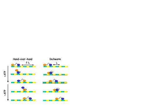
Figure 1: (Color online) Schematic representation of the possible mechanisms of motion for the motor of kinesin. In the hand-over-hand case each head moves a distance equals to $2l_{0}$ whereas in the inchworm the period of motion is $l_{0}$.

Two strategies can be devised in order to model the motion of molecular motors Fisher ; Chow . On one hand continuous models based on mirror symmetry breaking potentials (ratchet potentials Reimann ) or time symmetry broken driven forces Chacon . On the other hand, discrete kinetics models which are based on the solution of master equations associated to different states of the motor (see Fisher and references therein). Using either approximation both mechanisms have been studied: inchworm Cilla ; Sancho2 or hand-over-hand SaoGao ; Ping ; Sancho1 ; Sasaki .

In this work we study a minimalist mechanical continuous model for hand-over-hand motion that, we believe, captures the main features of biological motors. The model also has into account the properties of the microtubule substrate. The article is organised as follows: first we cast a two dimensional model which can mimic the motion of the motor. Within of reasonable values of parameters we explore different regimes of motion. In the conclusions section we will discuss the validity of the results to model a molecular motor.

II 2-D MODEL

In order to find a suitable model for the kinesin motor, its properties shall be studied carefully. Ref. Carter summarizes all these features: kinesin is a two-head protein which moves along the microtubule with $8.3\,nm$ steps, matching the repeat distance of the microtubule lattice; each step needs 1 ATP which is hydrolyzed and the movement stalls when a backward load of $7\,pN$ is applied. Experiments reported in Yildiz show, by marking one of the heads, that the motion follows the hand-over-hand mechanism, as a $16.6\,nm$ step is observed for each head, thus forbidding the movement proposed in the inchworm mechanism.

The description of the movement is rather simple: the two heads of the kinesin are attached to the microtubule Mori in two neighbor monomers until 1 ATP molecule is hydrolyzed by the head backwards. This energy frees the head, which moves to a new binding place ahead the other one. Two complementary mechanisms to understand how the particle released is able to find the next binding site have been proposed Carter ; Tomi : (a) The neck linker mechanism assumes a conformational change in the neck between heads which moves the free head from one place to the next forwards. (b) The diffusional search relies on the assumption that the noise associated to the thermal bath that surrounds the particle makes the free particle move, and this movement is preferably forwards and forced by the particle ahead which is attached to the microtubule.

Thermal fluctuations play a central role in the whole process. In the nanometer-length dimension and at room temperature, motion is governed by randomness induced by the environment (in this case the cytosol, made up mainly by water). At this scale damping and thermal noise are dominant and the dynamics can be studied by an overdamped Langevin equation:

$$\gamma\frac{d{\bf r}}{dt}=-{\bf\nabla}V({\bf r})+{\bf F}({\bf r},t)+{\bm{\xi}}(t).$$ (1)

Here ${\bf F}$ stands for external forces and ${\bm{\xi}}$ for thermal noise, being

$$<\xi_{j}(t)\xi_{k}(t^{\prime})>=2\,\gamma\,k_{B}\,T\,\delta(t-t^{\prime})\delta_{jk}$$ (2)

($\xi_{j}$ and $\xi_{k}$ are Cartesian components of the vector ${\bm{\xi}}$).

II.1 Energy potentials

We will model the kinesin as two interacting particles moving in the plane under the effect of flashing ratchet substrate potentials (two particles moving in two dimensions).

The potential energy of the system is given by

$$V({\bf r_{1}},{\bf r_{2}})=V_{1}({\bf r_{1}},t)+V_{2}({\bf r_{2}},t)+V_{12}({\bf r_{1}}-{\bf r_{2}})$$ (3)

The two heads of the kinesin are linked through a modified version of the Finite Extensible Non-linear Elastic (FENE) interaction FENE :

$$V_{12}(r)=-\,\frac{1}{2}K\,R_{0}^{2}\,\log\left(1-\frac{(r-l_{0})^{2}}{R_{0}^{2}}\right),$$ (4)

with $r=|{\bf r_{1}}-{\bf r_{2}}|$, $K$ is the stiffness of the neck, $l_{0}$ the equilibrium distance between heads and $R_{0}$ determines a maximum allowed separation, $l_{0}-R_{0}<r<l_{0}+R_{0}$.

With respect to the substrate potentials, in order to model the characteristics observed, two periodic flashing ratchet potentials lagged half a period in the $x$ direction will be used.

$$V_{j}({\bf r},t)=V_{j}({\bf r})f_{j}(t).$$ (5)

$j=1,2$ and in the $x$ direction the potentials are periodic with period $2l_{0}$ and $V_{2}$ is displaced $l_{0}$, the period of the microtubule lattice l0 , with respect to $V_{1}$:

$$V_{1}({\bf r}+2l_{0}{\bf\hat{x}})=V_{1}({\bf r})=V_{2}({\bf r}+l_{0}{\bf\hat{x}}).$$ (6)

The mathematical description of the 2d potential associated to particle 1 [see Fig. (2)] is the following

$$V_{1}(x,y)=V_{1x}(x)+V_{1y}(y)$$ (7)

with

$$V_{1x}(x)=\left\{\begin{array}[]{clc}\frac{x}{x_{M}}V_{0}&{\rm if}&0\leq x\leq x_{M}\\ \\ \frac{2l_{0}-x}{2l_{0}-x_{M}}V_{0}&{\rm if}&x_{M}\leq x\leq 2l_{0}.\\ \end{array}\right.$$ (8)

$x_{M}$ controls the asymmetry of the potential and if $x_{M}=l_{0}$ the potential is symmetric.

In order to confine the particles in the microtubule channel, with respect to the $y$ direction we choose a simple parabolic dependence.

$$V_{1y}(y)=\frac{1}{2}k_{y}\cdot y^{2}$$ (9)

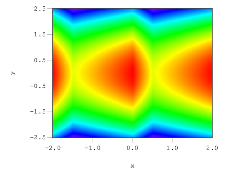
Figure 2: (Color online) Surface plot of the 2d substrate potential $V_{1}$. Minima correspond to $\widetilde{x}=2n$ ($n=0,\pm 1,...$) and $\widetilde{y}=0$.

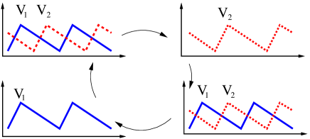
Figure 3: (Color online) Time sequence for the flashing ratchet substrate potentials. Each potential acts on a different particle. Note that this potential follows the sequence of attach-deattach shown in the hand-over-hand motion, Fig. 1.

We still have to define $f_{j}(t)$. The idea is to reproduce a cyclic motion. Such a cycle has 4 steps, see Fig. (3. First ($t=0$) both particles are confined close to the minima of their respective potentials and thus separated an averaged distance $l_{0}$ (the natural length of the neck). After a given time $t_{\rm on}$ some energy arrives at particle 1 for instance which does not see its substrate potential for a time $t_{\rm off}$. During this time this particle suffer a thermal diffusion only subjected to the interaction with the other particle. When $V_{1}$ is switched on again at $t=t_{\rm on}+t_{\rm off}$, the particle slides down towards some minimum energy position. This step lasts another $t_{\rm on}$ time and then at $t=2t_{\rm on}+t_{\rm off}$, $V_{2}$ is switched off for a $t_{\rm off}$ time closing the cycle. The total period of this cycle is $T=2t_{\rm on}+2t_{\rm off}$. As we will see, thanks to the asymmetric character of the potential a directed motion is obtained.

In order to compute the efficiency of the motion we define an efficiency parameter given by:

$$\varepsilon=\frac{\langle\Delta x_{1}\rangle}{2l_{0}}\times 100,$$ (10)

where $\langle\Delta x_{1}\rangle$ is the average advance of particle 1 (for instance) per cycle of the potential. Note that our definition of efficiency is basically the velocity of the motion, in fact the mean velocity can be computed as $v_{\rm mean}=\frac{\epsilon}{100}\times 2l_{0}/(t_{on}+t_{off})$ and is not related to the input of energy and the output of work.

The important parameter here is $t_{\rm off}$, the time a particle has for the diffusive motion. $t_{\rm on}$ only requires to be long enough to allow for relaxation towards a minimum, which in overdamped dynamics happens very fast. Thus, in our simulations we have played with different values of $t_{\rm off}$ and set $t_{\rm on}=t_{\rm off}$. This value corresponds to a duty ratio $r=t_{\rm on}/(t_{\rm on}+t_{\rm off})=0.5$ which guarantees the processivity of the motion Howard ; Chow .

II.2 Normalization

We will measure distance in units of $l_{0}=8.3$ nm, the distance between monomers in the microtubule, see also l0 . Energy is measured in units of $V_{0}$, the maximum value of the substrate potential. We choose $V_{0}\simeq E_{\rm ATP}\simeq 20$ $k_{B}T$ (at 300 K) com1 . The natural unit of time will be $\tau=l_{0}^{2}\gamma/V_{0}\simeq 40$ ns. Here, $\gamma$ is the damping coefficient used in the Langevin equation ($\gamma=6\pi\eta r=4.7\cdot 10^{-11}\frac{kg}{s}$, with $\eta=10^{-3}$ Pa the viscosity of the water and $r=25\,\AA$ the size of the head).

We will use now  $\widetilde{}$  signs for normalized variables as

$$\widetilde{x}=\frac{x}{l_{0}}\qquad;\qquad\widetilde{t}=\frac{t}{\tau}\quad;\qquad\widetilde{V}=\frac{V}{V_{0}}$$

$$\widetilde{T}=\frac{k_{B}\,T}{V_{0}}\qquad{\rm and}\qquad\widetilde{Q}=\frac{l_{0}\,Q}{V_{0}}$$ (11)

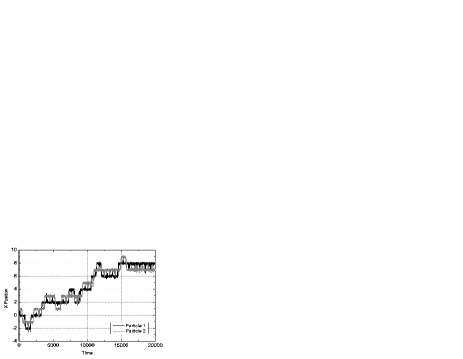
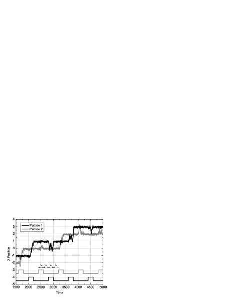
Figure 4: $\widetilde{x}$($\widetilde{t}$) for the two particles (top and middle) and trajectory in the $\widetilde{x}$–$\widetilde{y}$ plane (bottom). The middle figure also shows the flashing dynamics of the substrate potentials (the base lines correspond to the on periods).

III RESULTS

We are going to present our results based in the numerical integration of the normalised system of equations for the two particles. The integration algorithm we use is a version of the Runge-Kutta algorithm for integration of stochastic differential equations ($3_{O}\,4_{S}\,2_{G}$) sde1 ; sde2 . With respect to the different constants and parameters, unless extra information is given, the default normalized parameters will be we $\widetilde{T}=0.05$ (300 K), $\widetilde{t}_{\rm off}=\widetilde{t}_{\rm on}=20$, $\widetilde{K}=10$, $\widetilde{k}_{y}=1$, $\widetilde{R}_{0}=0.4$ and $\widetilde{x}_{M}=0.5$.

III.1 Dynamics of the system

Fig. 4 shows a typical example of the dynamics of the system at the parameter values listed above. There we can see that simulations reproduce the expected mechanism, a hand-over-hand net advance of the molecule. Middle figure shows a detail of the top one.

If both potentials are on, the particles do random motions around the minimum potential energy position. However, as one of the potentials is turned off, its linked particle starts to diffuse in 2d. The importance of the asymmetric mechanism is fully understood here. After $t_{\rm off}$, when the potential is turned on again, most of the times the particle is sited to the right of the maximum of the asymmetric potential and then typically moves down to the nearest minimum position. As we have said, due to the asymmetry of the potential, this minimum more frequently corresponds to the one to the right of the original one. Clearly, the more asymmetric the potential is, the more likely the system moves forward.

In the third graph of Fig. 4 we show the trajectories of the particles in phase space. The distance between heads moves around the rest distance $l_{0}$. Motion in the $x$ direction happens usually when one of the substrate potentials is off. Otherwise particles stay most of the time close to minimum energy position.

III.2 Efficiency as a function of $t_{\rm off}$ and $T$

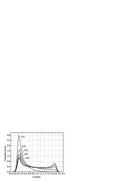
Figure 5: x-axis projection, at different normalized times $\widetilde{t}$, of the diffusion of a particle attached to the other, fixed at $(1,0)$, when no substrate potential is being applied. Data obtained at $\widetilde{T}=0.05$

A first estimation of the time needed for a particle to reach the next minimum can be easily worked out by using the 2D diffusion equation for the particle probability distribution $p(\varphi,t)$,

$$\frac{\partial p}{\partial t}=D\,\nabla^{2}p.$$ (12)

Writing [12] in polar coordinates and assuming that the distance between heads $r$ is constant the equation reads

$$\frac{\partial p}{\partial t}=\frac{D}{r^{2}}\,\left[\frac{\partial^{2}p}{\partial r^{2}}+\frac{1}{r}\,\frac{\partial p}{\partial r}+\frac{\partial^{2}p}{\partial\varphi^{2}}\right]_{r=const.}=\frac{D}{r^{2}}\frac{\partial^{2}p}{\partial\varphi^{2}}$$ (13)

This equation can be solved (making Fourier transformation for instance) with appropriated initial conditions

$$\left.p(\varphi,t)\right|_{t=0}=\delta(\varphi)$$ (14)

to give the normalized $p(\varphi,t)$

$$p(\varphi,t)=\frac{r}{2\sqrt{\pi\,D\,t}}\exp\left(\frac{-r^{2}\varphi^{2}}{4\,D\,t}\right)$$ (15)

from this results the mean angle reached at time $t$ is given by

$$\langle\varphi^{2}\rangle=\frac{2Dt}{r^{2}}=\frac{2k_{B}\,Tt}{\gamma r^{2}}$$ (16)

where we have used the Stokes-Einstein relation:

$$D=\frac{k_{B}\,T}{\gamma}.$$ (17)

Let be $\varphi_{M}$ the angle where the maximum of the potential is placed which is determined by the $x$ position of that maximum, $x_{M}$. If the particle is at a $x$ position less than $x_{M}$ when the potential turns on, it will return to its original position. However, if $x>x_{M}$ the particle will move forward. Assuming that the position of the maximum is placed at $\widetilde{x}_{M}=0.5$, and $\widetilde{r}=1$ we obtain $\varphi_{M}=\pi/3$. Figure 5 shows the time evolution of the probability distribution (projected on the x-axis). It is clearly observed that as time goes the probability of finding that a particle crosses the maximum $x_{M}$ increases. The time in which the probability for crossing is $1/2$ is simply given by

$$t=0.674\frac{r^{2}\varphi_{M}^{2}\gamma}{2k_{B}\,T}.$$ (18)

With the values given above the adimensional time (for temperature $\widetilde{T}=0.05$) is $\widetilde{t}\sim 16$. For this $t_{\rm off}$ time the efficiency of the motor is half of the maximum one, which is fixed by $x_{M}$ (see below).

Finally we analyze the behavior of the efficiency with temperature, Fig. 6. For low temperatures we need long $t_{\rm off}$ times to reach a reasonable efficiency as expected from equation [18] and we not get an asymptotic limit. For intermediate temperatures $\widetilde{T}=0.03-0.05$ the highest efficiency is achieved. Moreover, in the limit of high temperatures compared to the 2d potential and long $t_{\rm off}$, the efficiency starts to fall, as backwards movement is more likely to occur (the free particle can drag the confined one).

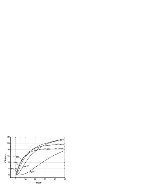
Figure 6: Efficiency as a function of $\widetilde{t}_{\rm off}$ for different normalized temperatures $\widetilde{T}$.

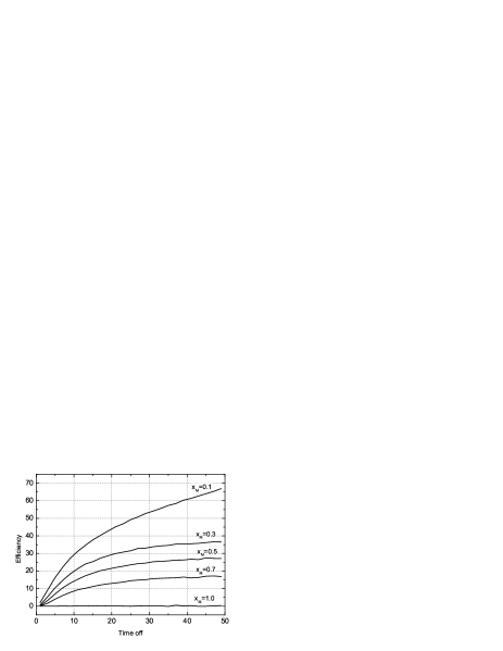
Figure 7: Efficiency as a function of $\widetilde{t}_{\rm off}$ at different positions of the maximum $\widetilde{x}_{M}$. When $\widetilde{x}_{M}=1.0$, the potential becomes symmetric and no rectified movement is observed.

III.3 Efficiency at different asymmetries

Here we present results on the behavior of the system as the asymmetry of the potential changes, being $x_{M}$ the parameter that controls it ($x_{M}$ fixes the position of the maximum in the period $2l_{0}$ periodic potential, so $\widetilde{x}_{M}=1$ corresponds to the symmetric case). At a given $t_{\rm off}$ time, efficiency depends importantly on this parameter. The mechanism will be inefficient for a symmetric potential and the largest efficiency will be obtain for the more asymmetric one.

Fig. 7 shows the numerical simulation of the efficiency as a function of $t_{\rm off}$ for different values of $x_{M}$. As we reduce the asymmetry the efficiency tends to zero, as shown in the $\widetilde{x}_{M}=1.0$ line, which corresponds to a symmetric potential. On the other hand the efficiency of the mechanism increases as we make the potential more asymmetric. In all the cases, when we increase $t_{\rm off}$ the efficiency grows from zero and saturates at its maximum value for long enough values of this parameter.

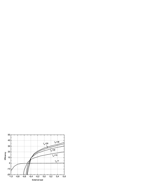
Figure 8: Efficiency as a function of the external load applied, $\widetilde{Q}$. Each line refers to a different $\widetilde{t}_{\rm off}$.

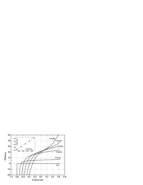
Figure 9: Efficiency as a function of the external load applied $\widetilde{Q}$, for different normalized temperatures $\widetilde{T}$.

III.4 Dynamics under external loads

In this section we want to explore the experimental results reported in Ref. Carter , where backward stepping was observed when using high backward loads. Then, it is worth studying how the system behaves under the effect of an external force.

To model the effect of such a load is not trivial. We have to decide how the total load $Q$ is divided into the two heads of the protein. It seems obvious that a head can make an opposite force to the applied only in case it is fixed to the microtubule. Therefore, the following mechanism is proposed: if there is only one head with its potential switched on, it will bear the whole opposite load. On the other hand, if both heads have their potential on, everyone will bear a force $Q/2$.

The expected behavior of the system is the following: as one potential turns off, its associated head starts diffusing. The other particle feels a force $Q$ which doubles the previous $Q/2$. Therefore, if that force is strong enough. the particle starts climbing the potential slope. The asymmetric potential plays again an important role: if the external force is positive, the particle faces the sharpest slope of the potential, so a bigger force than in the negative case is needed.

Fig. 8 shows the relationship between external load and $t_{\rm off}$. The most important characteristic is the value of the load for which the system does not move, 0 efficiency. For negative loads, as $t_{\rm off}$ shortens, the particle needs greater forces to start to move backwards. On the other hand, when long times are employed, the mechanism seems to reach a limit around $\widetilde{Q}=-0.5$.

We have also studied the effect of the temperature in the mechanism. Results are shown in Fig. 9 where efficiency versus external load for a given value of $\widetilde{t}_{\rm off}=20$ is plotted at different temperatures. An almost linear relation between critical load and temperature is obtained in this range.

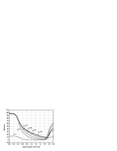
Figure 10: Efficiency as a function of the natural length of the neck, $\widetilde{l}_{0}^{\prime}$, for different values of $\widetilde{t}_{\rm off}$.

III.5 Varying the natural length of the neck

Up to now we have studied the case where the two space lengths of the system, the distance between monomers in the microtubule and the natural length of the neck, are equal (both are $l_{0}$). In this section we have extended our work to the study of the case when the natural distance between the heads is different from the spatial unit, fixed by the distance between monomers in the microtubule. Then, in our model, $l_{0}$ need to be replaced by $l_{0}^{\prime}$ in Eq. (4).

Fig. 10 is clear enough to provide strong evidence about the striking behavior observed as the natural length of the neck tends to 0: $100\%$ efficiency is achieved. This almost deterministic mechanism can be understood with the help of Fig. 11 and presents three steps: (a) We start with one particle sited in a minimum of the potential and the other one ahead (it feels a small force since the potential slope there is also small). (b) As the first potential disappears, the second particle moves to its minimum, dragging the other one. (c) Now the potential turns on, thus making the first particle to move ahead and we recover a situation equivalent to step (a).

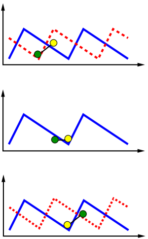
Figure 11: (Color online) Schematic explanation of the almost deterministic motion observed when $l_{0}^{\prime}$ close to zero.

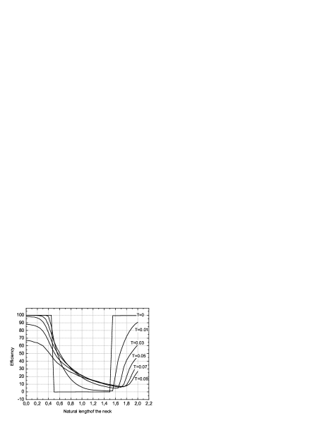
Figure 12: Efficiency versus $\widetilde{l}_{0}^{\prime}$ for different temperatures, $\widetilde{T}$.

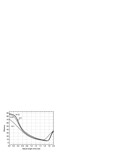
Figure 13: Efficiency versus $\widetilde{l}_{0}^{\prime}$ for different values of $\widetilde{K}$.

Fig. 12 shows results at different temperatures. First of all, the deterministic $T=0$ limit must be carefully explained. In this limit, there are only two possible values for the efficiency: $0\%$, associated to the range $\widetilde{l}_{0}^{\prime}\in\left(0.5,1.5\right)$, and $100\%$ for $\widetilde{l}_{0}^{\prime}\in\left[0.0,0.5\right)\cup\left(1.5,2.0\right]$. These two regions can be fully explained using the mechanism described above. In the $0\%$ case, switching off one of the potentials will make the other particle move to a minimum, but it will not be the minimum ahead which would not produce a net movement forwards.

There is just one parameter left to be discussed, which is the stiffness of the linker between heads of the motor. The study of the efficiency as a function of $l_{0}^{\prime}$ at different values of $K$ is shown in Fig. 13. For $\widetilde{l}_{0}^{\prime}<0.5$, the stiffness of the neck determines whether the particles prefer to be in their minimums no matter how far they are, or in an intermediate position, as plotted in Fig. 11 a).

IV CONCLUDING REMARKS

We have studied a simple mechanical model for hand-over-hand motion in two dimensions. This model has into account some important characteristics of two heads biological motor as kinesin. These characteristics are incorporated in the model in a simple but realistic way. The hand-over-hand mechanism requires a two-dimensional space. Unidirectionality is given by the ratchet potential in the advance direction. The balance between on and off times controls the efficiency and processivity of the motion. With all these ingredients we have been able to simulate the most remarkable features of kinesin motion within reasonable values of he parameters. Specifically, we have clearly observed a stochastic directed motion in which particles alternates each other (hand-over-hand). Moreover, a strong dependence of the stall force with off time and temperature has been found. Temperature makes a decrease of stall force with respect to one expected from energetic calculations. This decrease in the motor efficiency agrees with experimental observations Carter ; Fisher .

Several improvements to the model can be considered in future work. A link between $t_{\rm off}$ and ATP concentration could be established. This would imply a random flashing force instead of the periodic one used here. Another interesting extension of the model could allow the motor to change the lane in $y$ axis. This could be easily implemented by using a periodic potential in the transverse direction.

Finally, we have to stress that the characterization of the behavior and properties of those motors and the mechanisms behind them is an initial step toward the construction of synthetic nanoscale motors. This is a very active field in the nanoscience world. There has been some successful achievements in this field that include triptycene motors motor1 , helicene motors motor2 and a nanotube nanomotor nanotubo . In this article, we have shown the conditions for which a nanowalker can work.

- (1) M. Schliwa and G. Woehlke, Nature 422, 759 (2003).
- (2) M. G. L. van den Heuvel and C. Dekker, Science 317, 333 (2007).
- (3) R. D. Vale and R. A. Milligan, Science 288, 88 (2000).
- (4) J. Howard, Mechanics of Motor Proteins and the Cytoskeleton (Sinauer Associates 2001).
- (5) N. J. Carter and R. A. Cross, Nature 435, 308 (2005).
- (6) C. L. Asbury, Curr. Opin. Cell Biol. 17, 89 (2005).
- (7) F. Jülicher, Physica A 369, 185 (2006).
- (8) K. Visscher, M. J. Schnitzer and S. M. Block, Nature 400, 184 (1999).
- (9) F. Ritort, J. Phys.: Condens. Matter 18, R531 (2006).
- (10) A. Yildiz, M. Tomishige, R. D. Vale and P. R. Selvin, Science 303, 676 (2004).
- (11) C. L. Asbury, A. N. Fehr and S. M. Block, Science 302, 2130 (2003).
- (12) W. R. Schief, R. H. Clark, A. H. Crevenna and J. Howard, Proc. Natl. Acad. Sci. USA 101, 1183 (2004).
- (13) W. Hua, J. Chung and J. Gelles, Science 295, 844 (2002).
- (14) A. B. Kolomeisky and M. E. Fisher, Annu. Rev. Phys. Chem. 58, 675 (2007).
- (15) D. Chowdhury, arXiv:0709.1800v1 [physics.bio-ph] (2007).
- (16) P. Reimann, Phys. Rep. 361, 57 (2002).
- (17) R. Chacón and N. R. Quintero, Biosystems 88, 308 (2007).
- (18) S. Cilla, F. Falo and L. M. Floría, Phys. Rev. E 63, 031110 (2001).
- (19) A. Ciudad, J. M. Sancho, A. M. Lacasta, Physica A - Stat. Mech. and its Appl. 371, 25 (2006).
- (20) R. Kanada and K. Sasaki, Phys. Rev. E 67, 061917 (2003).
- (21) A. Ciudad, J. M. Sancho and G. P. Tsironis J. of Biol. Phys. 32, 455 (2007).
- (22) X. Ping, S. X. Dou and P. Y. Wang, Chinese Phys. 13, 1569 (2004).
- (23) Q. Shao, Y. Q. Gao, Proc. Nat. Acad. Sciences 103, 8072 (2006).
- (24) The point on if one or two heads are bounded to the microtubule in the rest state is controversial. A recent paper [T. Mori, R. D. Vale and M. Tomishige, Nature 459, 750 (2007)] supports both scenarios depending on the ATP concentration. In our model we assume that, in the rest state, the two heads are bounded to the microtubule, a situation which would correspond to a large ATP concentration. In any case, this is still an open question, see S. M. Block, Biophys. J. 92, 2986 (2007) for further discussions.
- (25) M. Tomishige, N. Stuurman and R. D. Vale, Nat. Struct. Mol. Biol. 13, 887 (2006).
- (26) K. Kremer, G. S. Grest, J. Chem. Phys. 92, 5057 (1990).
- (27) Note that at the moment we are using the same constant for the natural length of the neck, Eq. (4), and the period of the microtubule lattice, Eq. (6). This constraint will be relaxed later in section III-E.
- (28) As the ATP gives to the head the energy needed to jump over the potential barrier, the amplitude of the X-potential can be taken to be the energy extracted from a single ATP molecule, [Looking at biophysics , at room temperature, , therefore, ]. As the external load needed to make the system go backward is known, it can be also used to fix , as this force is used in making the particle climb over the smoothest slope of the potential considered. Therefore, using , which makes the slope considered be meters width, , and . The external load needed to stall the system and make it go backward has been experimentally measured in Carter , obtaining .
- (29) E. Helfand, Bell System Technical Journal 58, 2289 (1979).
- (30) H. S. Greensidea and E. Helfand. The Bell System Technical Journal 60, 1927 (1981).
- (31) Philip Nelson, Biological Physics: Energy, Information, Life (W. H. Freeman and Co., 2004).
- (32) N. Koumura, R, W. J. Zijlstra, R. A. van Delden, N. Harada and B. L. Feringa, Nature 401, 152 (1999).
- (33) T. R. Kelly, H. de Silva, R. A. Silva, Nature 401, 150 (1999).
- (34) A. M. Fennimore, T. D. Yuzvinsky, W. Q. Han, M. S. Fuhrer, J. Cumings and A. Zettl, Nature 424, 408 (2003).