Chi-square simulation of the CIR process and the Heston model

Abstract

The transition probability of a Cox–Ingersoll–Ross process can be represented by a non-central chi-square density. First we prove a new representation for the central chi-square density based on sums of powers of generalized Gaussian random variables. Second we prove Marsaglia’s polar method extends to this distribution, providing a simple, exact, robust and efficient acceptance-rejection method for generalized Gaussian sampling and thus central chi-square sampling. Third we derive a simple, high-accuracy, robust and efficient direct inversion method for generalized Gaussian sampling based on the Beasley–Springer–Moro method. Indeed the accuracy of the approximation to the inverse cumulative distribution function is to the tenth decimal place. We then apply our methods to non-central chi-square variance sampling in the Heston model. We focus on the case when the number of degrees of freedom is small and the zero boundary is attracting and attainable, typical in foreign exchange markets. Using the additivity property of the chi-square distribution, our methods apply in all parameter regimes.

1 Introduction

The mean-reverting square-root process or Cox–Ingersoll–Ross (CIR) process is frequently used in finance and economics to model the evolution of key financial variables, most notably to model the short rate of interest (Cox, Ingersoll and Ross CIR ) and in the Heston stochastic volatility model (Heston H ). Other applications include the modelling of mortality intensities and of default intensities in credit risk models, for example. The CIR process can be expressed in the form

$$\mathrm{d}V_{t}=\kappa(\theta-V_{t})\,\mathrm{d}t+\varepsilon\sqrt{V_{t}}\,\mathrm{d}W^{1}_{t},$$

where $W^{1}$ is a Wiener process and $\kappa$, $\theta$ and $\varepsilon$ are positive constants. The Heston model is a two-factor model, in which one component $S$ describes the evolution of a financial variable such as a stock index or exchange rate, and another component $V$ describes the stochastic variance of its returns. Indeed the stochastic variance $V$ evolves according to the CIR process described above. The Heston model is then completed by prescribing the evolution of $S$ by

$$\mathrm{d}S_{t}=\mu S_{t}\,\mathrm{d}t+\sqrt{V_{t}}\,S_{t}\,\bigl{(}\rho\,\mathrm{d}W^{1}_{t}+\sqrt{1-\rho^{2}}\,\mathrm{d}W^{2}_{t}\bigr{)},$$

where $W^{2}_{t}$ is an independent scalar Wiener process. The additional parameter $\mu$ is positive, while $\rho\in(-1,1)$.

The transition probability density of the CIR process is known explicitly, it can be represented by a non-central chi-square density. Depending on the number of degrees of freedom $\nu\coloneqq 4\kappa\theta/\varepsilon^{2}$, there are fundamental differences in the behaviour of the CIR process. If $\nu$ is larger or equal to 2, the zero boundary is unattainable; if it is smaller than 2, the zero boundary is attracting and attainable. At the zero boundary though, the solution is immediately reflected into the positive domain. This behaviour in the latter case is particularly difficult to capture numerically.

A number of successful simulation schemes have been developed for the non-attainable zero boundary case. There are schemes based on implicit time-stepping integrators, see for example Alfonsi Al2005 , Kahl and Schurz KS and Dereich, Neuenkirch and Szpruch DNS . Other time discretization approaches involve splitting the drift and diffusion vector fields and evaluating their separate flows (sometimes exactly) before they are recomposed together, typically using the Strang ansatz. See for example Higham, Mao and Stuart HMS and Ninomiya and Victoir NV . However, these splitting methods and the implicit methods only apply in the non-attracting zero boundary case. Recently, Alfonsi Al2007 has combined a splitting method with an approximation using a binary random variable near the zero boundary to obtain a weak approximation method for the full parameter regime. Moro and Schurz MS have also successfully combined exponential splitting with exact simulation. Dyrting Dy outlines and compares several different series and asymptotic approximations for non-central chi-square distribution.

Other direct discretization approaches, that can be applied to the attainable and unattainable zero boundary case are based on forced Euler-Maruyama approximations and typically involve negativity truncations; some of these methods are positivity preserving. See for example Deelstra and Delbaen DD , Bossy and Diop BD and also Berkaoui, Bossy and Diop BBD , Lord, Koekkoek and Van Dijk LKVD , as well as Higham and Mao HM , among others. These methods all converge to the exact solution, but their rate of strong convergence and discretization errors are difficult to establish. The full truncation method of Lord, Koekkoek and Van Dijk LKVD has in practice shown to be the leading method in this class.

Exact simulation methods typically sample from the known non-central chi-square distribution $\chi_{\nu}^{2}(\lambda)$ for the transition probability of the CIR process $V$ (see Cox, Ingersoll and Ross CIR and Glasserman (Glass, , Section 3.4)). Broadie and Kaya BK proposed sampling from $\chi_{\nu}^{2}(\lambda)$ as follows. When $\nu>1$, $\chi_{\nu}^{2}(\lambda)=\bigl{(}\text{N}(0,\sqrt{\lambda})\bigr{)}^{2}+\chi_{\nu-1}^{2}$, so such a sample can be generated by a standard Normal sample and a central chi-square sample. When $0<\nu<1$, such a sample can be generated by sampling from a Poisson distribution with mean $\lambda/2$, and then sampling from a central $\chi_{2N+\nu}^{2}$ distribution.

In the Heston model, to simulate the asset price Broadie and Kaya integrated the variance process $V$ to obtain an expression for $\int\sqrt{V_{\tau}}\,\mathrm{d}W_{\tau}$. They substituted that expression into the stochastic differential equation for $\ln S_{t}$. The most difficult task left is then to simulate $\int V_{\tau}\,\mathrm{d}\tau$ on the global interval of integration conditioned on the endpoint values of $V$; see Smith Smith . The Laplace transform of the transition density for this integral is known from results in Pitman and Yor PY . Broadie and Kaya used Fourier inversion techniques to sample from this transition density. Glasserman and Kim GK on the other hand, showed that linear combinations of series of particular gamma random variables exactly sample this density. They used truncations of those series to generate suitably accurate sample approximations. Their method has proved to be highly effective in applications that do not require the simulation of intermediate values of the process $S$, for example when pricing derivatives that are not path-dependent. Anderson An suggested two approximations that make simulation of the Heston model very efficient, and allow for pricing path-dependent options. The first was, after discretizing the time interval of integration for the price process, to approximate $\int V_{\tau}\,\mathrm{d}\tau$ on the integration subinterval by a trapezoidal rule. This would thus require non-central $\chi_{\nu}^{2}(\lambda)$ samples for the volatility at each timestep. The second was to approximate and thus efficiently sample the $\chi_{\nu}^{2}(\lambda)$ distribution—in two different ways depending on the size of $\lambda$. Haastrecht and Pelsser HP have recently introduced a rival $\chi_{\nu}^{2}(\lambda)$ sampling method to Andersen’s which utilizes, for small $\lambda$, pre-caching tables for central chi-square $\chi^{2}_{\nu+2N}$ distributions for small values of $N$, and for large $\lambda$, a matched squared normal random variable.

There are also numerous approximation methods based on the corresponding Kolmogorov or Fokker–Planck partial differential equation. These can take the form of Fourier transform methods—see Carr and Madan CM , Kahl and Jäckel KJ2 or Fang and Oosterlee FO1 ; FO2 for example—or some involve direct discretization of the Kolmogorov equation—see in ’t Hout and Foulon Karel and Haentjens and in ’t Hout HHW_karel .

We focus on the challenge of the attainable zero boundary case and in particular on the case when $\nu\ll\,1$, typical of FX markets and long-dated interest rate markets as remarked in Andersen An , and also observed in credit risk, see Brigo and Chourdakis BC . (Using the additivity property of the chi-square distribution $\chi^{2}_{\nu+k}=\chi^{2}_{\nu}+\chi^{2}_{k}$, the results can be straightforwardly extended to all parameter regimes.) The method we propose follows the lead of Andersen An , we approximate the integrated variance process $\int V_{\tau}\,\mathrm{d}\tau$ by a trapezoidal rule. For the simulation of the non-central $\chi_{\nu}^{2}(\lambda)$ transition density of the CIR process that is used to model the variance process required for each timestep of this integration method, we suggest two new methods that rely on the following representation. A non-central $\chi_{\nu}^{2}(\lambda)$ random variable can be generated from a central $\chi_{2N+\nu}^{2}$ random variable with $N$ chosen from a Poisson distribution with mean $\lambda/2$. Further, a $\chi_{2N+\nu}^{2}$ random variable can be generated from the sum of squares of $2N$ independent standard Normal random variables (more efficiently sampled as the sum of the logarithm of $N$ uniform random variables) and an independent central $\chi_{\nu}^{2}$ random variable. So the question we now face is how can we efficiently simulate a central $\chi_{\nu}^{2}$ random variable, especially for $\nu<1$? Suppose that $\nu$ is rational and expressed in the form $\nu=p/q$ with $p$ and $q$ natural numbers. We show that a central $\chi_{\nu}^{2}$ random variable can be generated from the sum of the $2q$th power of $p$ independent random variables chosen from a generalized Gaussian distribution $\text{N}(0,1,2q)$.

The question now becomes, how can we sample from a $\text{N}(0,1,2q)$ distribution? We have two answers. The first lies in generalizing Marsaglia’s polar method for pairs of independent standard Normal random variables, which we call the Marsaglia generalized Gaussian method (MAGG). The second method generalizes the Beasley–Springer–Moro direct inversion method for standard Normal random variables to generate a high accuracy approximation of the inverse generalized Gaussian distribution function. We provide a thorough comparison, of our generalized Marsaglia polar method and of our direct inversion method for sampling from the central $\chi_{\nu}^{2}$ distribution, to the acceptance-rejection methods of Ahrens–Dieter and Marsaglia–Tsang (see Ahrens and Dieter AD:chi , Glasserman Glass and Marsaglia and Tsang MarTsa ).

The CIR process can thus be simulated by the two approaches just described; exactly in the first instance and with very high accuracy in the second. The advantages of both approaches are that for the mean-reverting variance process in the Heston model, we can efficiently generate high quality samples simply and robustly. The methods require the degrees of freedom to be rational, however this is fulfilled in practical applications: the parameter $\nu$ will typically be obtained through calibration and can only be computed up to a pre-specified accuracy. We demonstrate our two methods in the computation of option prices for parameter cases that are considered in Andersen An and Glasserman and Kim GK and described there as challenging and practically relevant. We also demonstrate our methods for the pricing of path-dependent derivatives.

To summarize, we:

• Prove that a central chi-squared random variable with less than one degree of freedom, can be written as a sum of powers of generalized Gaussian random variables;

• Prove a new method—the generalized Marsaglia polar method—for generating generalized Gaussian samples;

• Provide a new and fast high-accuracy approximation (in principle to machine error) to the inverse generalized Gaussian distribution function;

• Establish two new simple, flexible, high-accuracy, efficient methods for simulating the Cox–Ingersoll–Ross process, for an attracting and attainable zero boundary, which we apply to simulating the Heston model.

Our paper is organised as follows. In Section 2 we present our new generalized Marsaglia method and our direct inversion method for sampling from the generalized Gaussian distribution. In Section 3 we derive the representation of a chi-square distributed random variable as a sum of powers of independent generalized Gaussian random variables. We include a thorough comparison of the generalized Marsaglia method and the direct inversion method for the central chi-squared distribution (based on sampling from the generalized Gaussian distribution) with the acceptance-rejection methods of Ahrens and Dieter AD:chi and of Marsaglia and Tsang MarTsa . We apply both our methods to the CIR process and Heston model in Section 4. We compare their accuracy and efficiency to the leading approximation method of Andersen An . Finally in Section 5 we present some concluding remarks.

2 Generalized Gaussian sampling

We require an efficient method for generating generalized Gaussian samples. Here we provide two such methods. The first method is a generalization of Marsaglia’s polar method for standard Normal random variables. This is an exact acceptance-rejection method. The second method is a direct inversion method that generalizes the Beasley–Springer–Moro method for standard Normal random variables. In principle this method is accurate to machine error.

Definition 1 (Generalized Gaussian distribution)

A generalized $\mathrm{N}(0,1,q)$ random variable, for $q\geqslant 1$, has distribution function for $x\in\mathbb{R}$:

$$\Phi(x)\coloneqq\gamma_{q}\int_{-\infty}^{x}\exp\bigl{(}-|\tau|^{q}/2\bigr{)}\,\mathrm{d}\tau,$$

where $\gamma_{q}\coloneqq q/\bigl{(}2^{1/q+1}\Gamma(1/q)\bigr{)}$ and $\Gamma(\cdot)$ is the standard gamma function.

See Gupta and Song GS , Song and Gupta SG , Sinz, Gerwinn and Bethge SGB , Sinz and Bethge SB and Pogány and Nadarajah PN for more details on this distribution and its properties.

2.1 Generalized Marsaglia polar method

We generalize Marsaglia’s polar method for pairs of independent standard Normal random variables (see Marsaglia Mar ).

Theorem 2.1 (Generalized Marsaglia polar method)

Suppose for some $q\in\mathbb{N}$ that $U_{1},\ldots,U_{q}$ are independent identically distributed uniform random variables over $[-1,1]$. Condition this sample set to satisfy the requirement $\|U\|_{q}<1$, where $\|U\|_{q}$ is the $q$-norm of $U=(U_{1},\ldots,U_{q})$. Then the $q$ random variables generated by $U\cdot(-2\log\|U\|_{q}^{q})^{1/q}/\|U\|_{q}$ are independent $\text{N}(0,1,q)$ distributed random variables.

Proof

Suppose for some $q\in\mathbb{N}$ that $U=(U_{1},\ldots,U_{q})$ are independent identically distributed uniform random variables over $[-1,1]$, conditioned on the requirement that $\|U\|_{q}<1$. Then the scalar variable $Z\coloneqq(-2\log\|U\|_{q}^{q})^{1/q}>0$ is well defined. Let $f$ denote the probability density function of $U$ given $\|U\|_{q}<1$; it is defined on the interior of the $q$-sphere, $\mathbb{S}_{q}(1)$, whose bounding surface is $\|U\|_{q}=1$. We define a new set of $q$ random variables $W=(W_{1},\ldots,W_{q})$ by the map $G\colon\mathbb{S}_{q}(1)\to\mathbb{R}^{p}$ where $G\colon U\mapsto W$ is given by $G\circ U=(Z/\|U\|_{q})\cdot U$. Note that the inverse map $G^{-1}\colon\mathbb{R}^{p}\to\mathbb{S}_{q}(1)$ is well defined and given by $G^{-1}\circ W=Z^{-1}\cdot\exp(-Z^{q}/2q)\cdot W$, where we note that in fact $Z=\|W\|_{q}$ which comes from taking the $q$-norm on each side of the relation $W=G(U)$. We wish to determine the probability density function of $W$. Note that if $\Omega\subset\mathbb{R}^{q}$, then we have $\mathbb{P}\,\bigl{(}W\in\Omega\bigr{)}=\mathbb{P}\,\bigl{(}U\in G^{-1}(\Omega)\bigr{)}=\int_{G^{-1}(\Omega)}f\circ u\,\mathrm{d}u=\int_{\Omega}(f\circ G^{-1}\circ w)\cdot\bigl{|}\det(\mathrm{D}G^{-1}\circ w)\bigr{|}\,\mathrm{d}w$, where for $w=(w_{1},\ldots,w_{p})\in\Omega$, the quantity $\mathrm{D}G^{-1}\circ w$ denotes the Jacobian transformation matrix of $G^{-1}$. Hence the probability density function of $W$ is given by $(f\circ G^{-1}\circ w)\cdot\bigl{|}\det(\mathrm{D}G^{-1}\circ w)\bigr{|}$. The Jacobian matrix and its determinant are established by direct computation. For each $i,k=1,\ldots,q$ we see that if we define $g(z)\coloneqq-(1/2+1/z^{q})$, then

$$\partial G^{-1}_{k}/\partial w_{i}=z^{-1}\exp(-z^{q}/2q)\cdot\Bigl{(}\delta_{ik}+g(z)\cdot\bigl{(}\mathrm{sgn}(w_{i})\cdot|w_{i}|^{q-1}\bigr{)}\cdot w_{k}\Bigr{)},$$

where $\delta_{ik}$ is the Kronecker delta function. If we set $v=\bigl{(}\mathrm{sgn}(w_{1})\cdot|w_{1}|^{q-1},\ldots,\mathrm{sgn}(w_{q})\cdot|w_{q}|^{q-1}\bigr{)}^{\mathrm{T}}$ then we see that our last expression generates the following relation for the Jacobian matrix: $z\exp(z^{q}/2q)\cdot\bigl{(}\mathrm{D}G^{-1}\circ w\bigr{)}=I_{q}+g(z)\cdot v\,w^{\mathrm{T}}$, where $I_{q}$ denotes the $q\times q$ identity matrix. From the determinant rule for rank-one updates—see Meyer (Meyer, , p. 475)—we see that the determinant of the Jacobian matrix is given by

$$\det(\mathrm{D}G^{-1}\circ w\bigr{)} =z^{-q}\exp(-z^{q}/2)\cdot\bigl{(}1+g(z)\,w^{\mathrm{T}}\,v\bigr{)}$$

$$=z^{-q}\exp(-z^{q}/2)\cdot\bigl{(}1+g(z)\,z^{q}\bigr{)}$$

$$=-\tfrac{1}{2}\exp(-z^{q}/2).$$

Noting that $\mathrm{vol}\bigl{(}\mathbb{S}_{q}(1)\bigr{)}=2^{q}\cdot\bigl{(}\Gamma(1/q)\bigr{)}^{q}/q^{q}$ we have

$$(f\circ G^{-1}\circ w)\cdot\bigl{|}\det(\mathrm{D}G^{-1}\circ w)\bigr{|}=\frac{q^{q}}{2^{q+1}\bigl{(}\Gamma(1/q)\bigr{)}^{q}}\cdot\exp(-z^{q}/2).$$

This is the joint probability density function for $q$ independent identically distributed $q$-generalized Gaussian random variables, establishing the required result. ∎

Remark 1

The corresponding generalization of the Box–Muller method involves the beta distribution, which does not appear to be a convenient approach; see Liang and Ng LNg , Harman and Lacko HL and Lacko and Harman LH .

2.2 Direct inversion method

We generalize the Beasley–Springer–Moro direct inversion method for standard Normal random variables to the generalized Gaussian $\text{N}(0,1,q)$ for $q>2$; see Moro Moro or Joy, Boyle and Tan JBT for the case $q=2$. We focus on the case of large $q$; the reasons for this will become apparent in Section 3. In the limit of large $q$ the probability density function for the generalized Gaussian attains the profile of the density of a $\text{U}(-1,1)$ uniform random variable. For large but finite $q$ the probability density function of the generalized Gaussian resembles a smoothed version of the $\text{U}(-1,1)$ density profile. It naturally exhibits three distinct behavioural regimes which are also naturally reflected in the generalized Gaussian distribution function $\Phi$, as well as its inverse $\Phi^{-1}$ which is our principal object of interest. We use the symmetry of the density function to focus on the positive half $[0,\infty)$ of its support. Correspondingly the inverse distribution function $\Phi^{-1}$ is anti-symmetric about $1/2$; and we can focus on the subinterval $[1/2,1)$ of its support. Since $\Phi$ is monotonic (and bijective) we naturally identify (and pairwise) label the three behavioural regimes of the density function and inverse distribution function as follows. We set $x_{*}\coloneqq\bigl{(}2(1-1/q)\bigr{)}^{1/q}$ and

$$x_{\pm}\coloneqq\Bigl{(}3(1-1/q)\pm\bigl{(}(5-1/q)(1-1/q)\bigr{)}^{1/2}\Bigr{)}^{1/q}$$

and correspondingly $\Phi_{*}\coloneqq\Phi(x_{*})$ and $\Phi_{\pm}\coloneqq\Phi(x_{\pm})$. Here $x_{*}\in[0,\infty)$ denotes the inflection point of the density profile, i.e. $\Phi^{\prime\prime\prime}(x_{*})=0$, while $x_{\pm}\in[0,\infty)$ are the points where $\Phi^{\prime\prime\prime\prime}(x_{\pm})=0$. Then we identify the:

1. Central region where $x\in[0,x_{-}]$ or $\Phi\in[1/2,\Phi_{-}]$—roughly corresponding to the region where the density profile is flat and approximately equal to $1/2$;

2. Middle region where $x\in[x_{-},x_{+}]$ or $\Phi\in[\Phi_{-},\Phi_{+}]$—roughly corresponding to the region where the density profile has a large negative slope; and

3. Tail region where $x\in[x_{+},\infty)$ or $\Phi\in[\Phi_{+},1)$—roughly corresponding to the region where the density profile is flat and approximately equal to zero.

As in Beasley and Springer BS , in the central region we approximate the inverse generalized Gaussian $\Phi^{-1}=\Phi^{-1}(u)$ with $u\in[1/2,\Phi_{-}]$ by an $(m,n)$ Padé approximant

$$\Phi^{-1}(u)\approx U\cdot\frac{a_{0}+a_{1}(U^{q})+\cdots+a_{m}(U^{q})^{m}}{1+b_{1}(U^{q})+\cdots+b_{n}(U^{q})^{n}},$$

where $U=(u-1/2)/\gamma_{q}$, with $\gamma_{q}$ the reciprocal of the normalizing factor of the generalized Gaussian distribution, and $a_{0},\ldots,a_{m},b_{1},\ldots,b_{n}$ are constant coefficients. Typically across a large range of values of $q$ the choice of values for $m$ and $n$ equal to $3,4$ or $5$ generate approximations with order of $10^{-10}$ accuracy. The coefficients $a_{0},\ldots,a_{m}$ and $b_{1},\ldots,b_{n}$ change as $q$ varies—see the discussion below.

Motivated by the approximations suggested in Blair, Edwards and Johnson BEJ , in the middle region we approximate $\Phi^{-1}$ with $u\in[\Phi_{-},\Phi_{+}]$ by a rational $(m,n)$ Padé approximation of a scaled and shifted variable as follows:

$$\Phi^{-1}(u)\approx\frac{c_{0}+c_{1}(\eta-\eta_{*})+\cdots+c_{m}(\eta-\eta_{*})^{m}}{1+d_{1}(\eta-\eta_{*})+\cdots+d_{n}(\eta-\eta_{*})^{n}},$$

where $\eta\coloneqq-\log(1-u)$, $\eta_{*}\coloneqq-\log(1-\Phi_{*})$ and $c_{0},\ldots,c_{m},d_{1},\ldots,d_{n}$ are constant coefficients. Note that the integers $m$ and $n$ here are distinct from those in the central approximation above. Again typically as $q$ varies, values of $m$ and $n$ equal to $3,4$ or $5$ generate approximations with order of $10^{-10}$ accuracy.

Now using the ansatz of Moro Moro , in the tail region we approximate $\Phi^{-1}$ with $u\in[\Phi_{+},1)$ by a degree $n$ Chebychev polynomial approximation—suggested in Joy, Boyle and Tan JBT —of a scaled and shifted variable as follows:

$$\Phi^{-1}(u)\approx\hat{c}_{0}T_{0}(z)+\hat{c}_{1}T_{1}(z)+\cdots+\hat{c}_{n}T_{n}(z)-\hat{c}_{0}/2$$

where $T_{n}$ is the degree $n$ Chebychev polynomial in $z\in[-1,1]$, where $z\coloneqq k_{1}\xi+k_{2}$ and $\xi\coloneqq\log\bigl{(}-\log\bigl{(}(1-u)/C_{q}\bigr{)}\bigr{)}$, with $C_{q}\coloneqq 1/\bigl{(}2\Gamma(1/q)\bigr{)}$. The parameters $k_{1}$ and $k_{2}$ are chosen so that $z=-1$ when $u=\Phi_{+}$ and $z=1$ when $u=1-10^{-12}$. Then as $q$ varies, values of $n$ equal to $10$ generate approximants with order $10^{-10}$ accuracy. As we discuss below, when we evaluate the Chebychev polynomials using double precision arithmetic, we need to restrict the tail approximation to $u\in[\Phi_{+},1-10^{-8}]$.

Remark 2

The choices of the scaled variables in the central and tail region approximations above are motivated by the asymptotic approximation for $\Phi^{-1}=\Phi^{-1}(u)$ as $u\to 1^{-}$. After applying the logarithm to the large $x$ asymptotic expansion for the generalized Gaussian distribution function $\Phi=\Phi(x)$, we get for $y\coloneqq x^{q}/2$:

$$y=-\log\biggl{(}\frac{1-\Phi(x)}{C_{q}}\biggr{)}+(1/q-1)\log y-y+\log\biggl{(}1+\sum_{n\geqslant 1}\frac{(1/q-1)\cdots(1/q-n)}{y^{n}}\biggr{)}.$$

We can generate an asymptotic expansion for $y$ and thus $\Phi^{-1}=(2y)^{1/q}$ by iteratively solving the above equation with initial guess given by the first term on the right shown above. The expansion is $y\sim\mathrm{e}^{\xi}+(1/q-1)\xi+\mathrm{e}^{-\xi}P_{1}(\xi)+\mathrm{e}^{-2\xi}P_{2}(\xi)+\cdots$, where the $P_{n}$ for $n\geqslant 1$ are explicitly determinable degree $n$ polynomials.

For some fixed values for $q$, we quote in Appendix B values for the coefficients for the approximations above in the three regions. We obtained the coefficients in the case of the two Padé rational approximants by applying the least squares approach advocated half way down page 205 in Press et al. PTVF . This requires values for $\Phi^{-1}$ at, for example, nodal points roughly distributed as zeros of a high degree Chebychev polynomial. These were obtained by high precision Gauss-Konrod quadrature approximation of $\Phi$ combined with a high precision root finding algorithm. In the case of the Chebychev approximations in the tail region, we computed the coefficients in the standard way, see for example Section 5.8 in Press et al. PTVF . Further Chebychev approximations can be efficiently evaluated using Clenshaw’s recurrence formula found on page 193 of Press et al.. Thus, with the $a$, $b$, $c$, $d$ and $\hat{c}$ coefficients above computed, our direct inversion algorithm is given in Appendix A.

Figure 1 shows the error in the inverse generalized Gaussian approximations for $q=10,100,1000$. The top three panels show that in all three cases, and across the central, middle and tail regions, the coefficients listed in Appendix B generate approximations with errors of order $10^{-10}$. This is comparable with the error in the Beasley–Springer–Moro approximation when $q=2$. We note the tail region we have considered extends to $1-10^{-8}$, whereas the tail region of Beasley–Springer–Moro extends to $1-10^{-12}$. The reason for this lies in the arithmetic precision we used. In fact we evaluated the coefficients for the Chebychev approximations in the tail regions using $25$ digit arithmetic, but evaluated the corresponding Chebychev polynomials in double precision arithmetic. Indeed in the top three panels in Figure 1, we can see the effect in tail regions of restricting calculations to double precision (16 digit) arithmetic. If we also evaluate the Chebychev polynomials in $25$ digit arithmetic then errors of our Chebychev polynomial approximations in the tail region are shown in the lower two panels in Figure 1. We observe there that our tail approximations in fact maintain $10^{-10}$ or better as far as $1-10^{-12}$ on the abscissa. However unless stated otherwise, all our subsequent calculations are performed using double precision arithmetic.

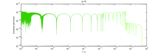
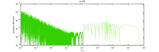
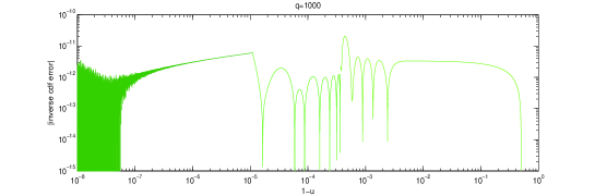
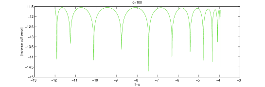
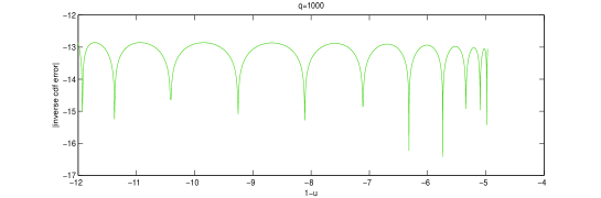
Figure 1: The top three panels show the error in our inverse generalized Gaussian distribution approximations, respectively for $q=10,100,1000$, computed using double precision arithmetic. Each panel shows the central, middle and tail approximants for the corresponding values of $q$. Note the error in all cases is of order $10^{-10}$. The lower two panels show the error in our tail approximations, respectively for $q=100,1000$, computed using 25 digit arithmetic.

3 Chi-square sampling

We begin by proving that random variables with a central $\chi_{\nu}^{2}$ distribution, especially for $\nu<1$, can be represented by random variables with a generalized Gaussian distribution.

Theorem 3.1 (Central chi-square from generalized Gaussians)

Suppose $X_{i}\sim\mathrm{N}(0,1,2q)$ are independent identically distributed random variables for $i=1,\ldots,p$, where $q\geqslant 1$ and $p\in\mathbb{N}$. Then we have

$$\sum_{i=1}^{p}\bigl{|}X_{i}\bigr{|}^{2q}\sim\chi_{p/q}^{2}.$$

Proof

If $X\sim\text{N}(0,1,2q)$, then we have $\mathbb{P}\bigl{(}|X|^{2q}<x\bigr{)}=2\cdot\mathbb{P}\bigl{(}0<X<|x|^{1/2q}\bigr{)}$ and a simple $2q$th power law transformation reveals that $|X|^{2q}\sim\chi_{1/q}^{2}$. Using that the sum of $p$ independent identically distributed $\chi_{1/q}^{2}$ random variables have a $\chi_{p/q}^{2}$ distribution establishes the result.∎

3.1 Generalized Marsaglia approach

We restrict ourselves to the case when the number of degrees of freedom is rational, i.e. $\nu=p/q$ with $p,q\in\mathbb{N}$. The algorithm for generating central $\chi_{\nu}^{2}$ samples is as follows.

Algorithm 1 (Exact central chi-square samples)

1. Generate $2q$ independent uniform random variables over $[-1,1]$: $U=(U_{1},\ldots,U_{2q})$.

2. If $\|U\|_{2q}<1$ continue, otherwise repeat Step 1.

3. Compute $Z=U\cdot(-2\log\|U\|_{2q}^{2q})^{1/2q}/\|U\|_{2q}$. This gives $2q$ independent $\text{N}(0,1,2q)$ distributed random variables $Z=(Z_{1},\ldots,Z_{2q})$.

4. Compute $Z_{1}^{2q}+\cdots+Z_{p}^{2q}\sim\chi_{p/q}^{2}$.

Remark 3

Note that if $p<2q$ then we can use the remaining $\text{N}(0,1,2q)$ random variables we generate in Step 3 the next time we need to generate a $\chi_{p/q}^{2}(\lambda)$ sample. In practice we don’t really need to consider the case $p\geqslant 2q$, but for the sake of completeness, we would simply generate $p-2q$ more $\text{N}(0,1,2q)$ samples by repeating Steps 1–3.

In Step 2, the probability of accepting $U_{1},\ldots,U_{2q}$ is given by the ratio of the volumes of $\mathbb{S}_{2q}(1)$ and $[-1,1]^{2q}$: $P_{\mathrm{Mar}}\coloneqq\bigl{(}\Gamma(1/2q)/2q\bigr{)}^{2q}$. Note for $q=1$, the probability of acceptance is 0.7854. Further as $q\to\infty$ we have $P_{\mathrm{Mar}}\to\exp(-\gamma)\approx 0.5615$. Here $\gamma$ is the Euler–Mascheroni constant and $\Gamma(z)\sim 1/z-\gamma$ as $z\to 0^{+}$.

In practice we will need to generate a large number of samples. For the generalized Marsaglia polar method, in each accepted attempt, we generate $2q$ generalized Gaussian random variables. Of these, $p$ random variables are used to generate a $\chi_{p/q}^{2}$ random variable. The number of attempts until the first success has a geometric distribution with mean $1/P_{\mathrm{Mar}}$. Hence the expected number of steps to generate $2q/p$ independent $\chi_{p/q}^{2}$ random variables is thus $1/P_{\mathrm{Mar}}$.

How does the acceptance rate of our central chi-squared sampling method based on the generalized Marsaglia polar method, for the case $\nu<2$, compare to the two leading acceptance-rejection methods? These are the methods of Ahrens and Dieter AD:chi (also see Glasserman (Glass, , pp. 126–7)) and the method of Marsaglia and Tsang MarTsa .

The acceptance-rejection algorithm of Ahrens–Dieter is based on a mixture of the prior densities $(\nu/2)\,x^{\nu/2-1}$ on $[0,1]$ and $\exp(1-x)$ on $(1,\infty)$, with weights $\mathrm{e}/(\mathrm{e}+\nu/2)$ and $(\nu/2)/(\mathrm{e}+\nu/2)$, respectively; here $\mathrm{e}=\exp(1)$. This method generates one $\chi_{\nu}^{2}$ random variable with probability of acceptance $P_{\mathrm{AD}}\coloneqq(\nu/2)\,\Gamma(\nu/2)\,\mathrm{e}/(\nu/2+\mathrm{e})$. In this method, the number of degrees of freedom $\nu$ can be any real number. The expected number of attempts to generate $2q/p$ independent $\chi_{p/q}^{2}$ distributed random variables is thus $(2q/p)\cdot(1/P_{\mathrm{AD}})$. How do the expected number of attempts compare? In other words, to generate $2q/p$ random variables, is $1/P_{\mathrm{Mar}}\leqslant(2q/p)\cdot(1/P_{\mathrm{AD}})$? Or equivalently, when does $p/q\leqslant 2P_{\mathrm{Mar}}/P_{\mathrm{AD}}$ hold? We examine the right-hand side more carefully; set $z\coloneqq 1/2q$, so $0<z<1/2$. Then we have

$$\frac{P_{\mathrm{Mar}}}{P_{\mathrm{AD}}}=\bigl{(}z\,\Gamma(z)\bigr{)}^{1/z}\cdot\frac{\nu/2+\mathrm{e}}{(\nu/2)\,\Gamma(\nu/2)\,\mathrm{e}}.$$

Note $z$ and $\nu/2$ are independent. A lower bound for $\bigl{(}z\,\Gamma(z)\bigr{)}^{1/z}$ is $\exp(-\gamma)\approx 0.5615$ for $0<z<1/2$, whilst a lower bound for $(\nu/2+\mathrm{e})/((\nu/2)\,\Gamma(\nu/2)\,\mathrm{e})$ is $1$ for $0<\nu<2$. Hence $2P_{\mathrm{Mar}}/P_{\mathrm{AD}}>1$ and so for $p/q<1$, the expected number of attempts for the generalized Marsaglia method is less than that for the Ahrens–Dieter method. We further note that the expected number of attempts for the generalized Marsaglia method to generate $2q/p$ chi-square samples is bounded by its value for $q=1$ and the limit as $q\to\infty$, more precisely the expected number of attempts is $1/P_{\mathrm{Mar}}\in(1.2732,\,1.7811)$. In contrast in the Ahrens–Dieter method, the expected number of attempts to generate $2q/p$ samples is $(2q/p)(1/P_{\mathrm{AD}})$, which is unbounded.

The expected number of steps is relevant in the context of how often an algorithm is called. The generalized Marsaglia method uses $2q$ uniform random variables each time it is called,   while the algorithm of Ahrens–Dieter requires only 2 random variables. The expected number of random variables required to generate $2q/p$ chi-square samples is thus $2q/P_{\mathrm{Mar}}$  and $4q/p\cdot 1/P_{\mathrm{AD}}$, respectively. Since

$$\frac{4q/p\cdot 1/P_{\mathrm{AD}}}{2q\cdot 1/P_{\mathrm{Mar}}}=\frac{2}{p}\cdot\frac{P_{\mathrm{Mar}}}{P_{\mathrm{AD}}}$$

and since $P_{\mathrm{Mar}}<P_{\mathrm{AD}}$, we see that the expected required number of input random variables is smaller for the generalised Marsaglia method for $p=1$ only, that is when the degrees of freedom can be written in the form $p/q=1/2q$.

Secondly, we compare the generalized Marsaglia method with the acceptance–rejection method of Marsaglia and Tsang MarTsa . Their method is based on taking  a transformation $h(X)=d(1+cX)^{3}$ on the set $\{X>-1/c\}$, where the distribution of $X$ is such that $h(X)$ has the required gamma distribution. Here $d=p/2q-1/3$ and $c=1/\sqrt{9d}$. The random variable $X$ can be sampled using an acceptance–rejection method based on sampling a Normal random variable. The acceptance probability is $P_{\mathrm{MT}}=\int_{-1/c}^{\infty}\mathrm{e}^{g(x)}\,\mathrm{d}x\,\cdot 1/\sqrt{2\pi}\cdot\bigl{(}1-\Phi(-1/c)\bigr{)}$, where

$$g(x)=d\ln\bigl{(}(1+cx)^{3}\bigr{)}-d(1+cx)^{3}+d$$

and where $\Phi$ denotes the standard Normal distribution function. The algorithm of  Marsaglia–Tsang assumes that the gamma parameter $p/2q\geq 1$. As noted there, a gamma random variable $\gamma(\alpha)$ with gamma parameter $\alpha<1$ can be generated by $\gamma(\alpha)=\gamma(1+\alpha)U^{1/\alpha}$, where $U\sim\text{U}(0,1)$. The acceptance probability $P_{\mathrm{MT}}$ can be numerically evaluated, for example, for $p/2q=1$ its value is $0.95167\cdot 0.992847=0.944864$, while for $p/2q=2$ its value is $0.98166\cdot 0.999946=0.98161$. By analogy to the comparison with the algorithm of Ahrens–Dieter above, we see that the expected number of steps to generate $2q/p$ independent $\chi^{2}_{p/q}$ random is smaller for the generalized Marsaglia method compared with the algorithm by Marsaglia and Tsang for $p<q$—the regime of interest here. The expected number of uniform random variables required to do this however is larger for the generalized Marsaglia method except if $p/q=1/2q$. We compare and discuss the numerical efficacy of both methods and of the algorithm of Ahrens and Dieter in Section 3.3 below.

3.2 Direct inversion

We restrict ourselves to case when the number of degrees of freedom $0<\nu<1$ is given to the first three decimal places and can thus be expressed in the form

$$\nu=\frac{p_{5}}{5}+\frac{p_{10}}{10}+\frac{p_{20}}{20}+\frac{p_{50}}{50}+\frac{p_{100}}{100}+\frac{p_{200}}{200}+\frac{p_{500}}{500}+\frac{p_{1000}}{1000}+\frac{p_{2000}}{2000},$$

for some $p_{q}\in\{0,1,2\}$ with $q\in\mathbb{S}$ where $\mathbb{S}=\{5,10,20,50,100,200,500,1000,2000\}$. For example, for $\nu=0.387$ we would have, since a $\text{N}(0,1,2q)$ random variable is needed to generate a $\chi_{1/q}^{2}$ one: $p_{10}=1$, $p_{20}=1$, $p_{50}=2$, $p_{500}=1$, $p_{1000}=1$ and $p_{2000}=1$, with the other $p_{q}$ coefficients equal to zero. Of course in principle we can extend our method to degrees of freedom $0<\nu<1$ given to any number of decimal places (see the discussion at the end of this section). In Appendix B we quote the coefficients and parameter values for Padé and Chebychev approximants required for direct inversion for the values of $q$ in $\mathbb{S}$. The algorithm for generating central $\chi_{\nu}^{2}$ samples, for any $\nu$ given to the first three decimal places, using direct inversion of generalized Gaussian samples is as follows.

Algorithm 2 (High accuracy central chi-square samples)

1. For each $q\in\mathbb{S}$, generate $p_{q}$ independent uniform random variables over $[0,1]$: $(U_{1,q},\ldots,U_{p_{q},q})$, i.e. a total of $\sum_{q\in\mathbb{S}}p_{q}$ independent uniform random variables.

2. For each $q\in\mathbb{S}$, use $(U_{1,q},\ldots,U_{p_{q},q})$ and the direct inversion algorithm in Appendix A to generate $p_{q}$ generalized Gaussian samples $(Z_{1,q},\ldots,Z_{p_{q},q})$.

3. Compute $\sum_{q\in\mathbb{S}}\sum_{k=1}^{p_{q}}Z_{k,q}^{2q}\sim\chi_{\nu}^{2}$.

Remark 4

We chose the set $\mathbb{S}$ and decomposition of $\nu$ above for efficiency and convenience. We could achieve greater efficiency by decomposing $\nu$ more finely, but this would increase the number of Padé and Chebychev approximants we need to compute and store.

3.3 Comparison

The natural question is how do the algorithms perform in practice? Two issues immediately surface. The first is that the generalized Marsaglia approach is restricted to rational numbers. In practical applications this is not restrictive as all finite precision arithmetic is in principle rational arithmetic. The second is that the direct inversion approach, as we have implemented it here, only allows for three decimal places. However, this is not a restriction either, as we can in principle construct additional approximations to the inverse generalized Gaussian distribution function for larger values of $q$. Indeed for $q=10^{4}$, we computed a $(3,1)$ Padé approximation for the central region, a $(4,5)$ Padé approximation for the middle region and a degree $10$ Chebychev approximation for the tail that guarantee accuracy of $10^{-9}$ across all regions for the inverse generalized Gaussian distribution function. We also note that parameter values are typically determined by calibration and quoted to only $2$ or $3$ significant figures.

Two leading gamma random variable acceptance-rejection sampling methods are those of Ahrens and Dieter AD:chi and Marsaglia and Tsang MarTsa . In Figure 2 we compare CPU times needed to generate $10^{5}$ samples versus the number of degrees of freedom $\nu$ using the generalized Marsaglia, Ahrens–Dieter, Marsaglia–Tsang and direct inversion methods. The values for the degrees of freedom chosen are $\nu=(1+m)\cdot 10^{-4}$ for $m=0,1,\ldots,1000$ and $\nu=0.101+m\cdot 10^{-3}$ for $m=0,1,\ldots,299$—we omitted CPU times for the direct inversion method involving the fourth decimal place. The CPU times were generated using compiled Matlab code to better reflect their potential practical implementations. We observe the Ahrens–Dieter and Marsaglia–Tsang acceptance-rejection methods roughly require the same CPU time to generate central $\chi_{\nu}^{2}$ samples for any of these values of $\nu$. The Ahrens–Dieter method also appears to be slightly more efficient. The generalized Marsaglia approach shows more variation in the CPU time required. In particular for example, for values of $\nu$ equal to $3$, $6$, $7$ and $9$ times $10^{-m}$ for all $m=2,3,4$, it takes longer to generate central $\chi_{\nu}^{2}$ samples than for the other $\nu$ values. This is due to the fact that as rational numbers, with denominators as powers of $10$, they do not simplify nicely to what might be considered the optimal format for sampling with this method, namely $1/2q$ (see also Section 3.1). For values of $\nu$ which cannot be reduced to this optimal format, we need to sum over a number of generalized Gaussian samples to produce a central $\chi_{\nu}^{2}$ sample. However any decimal with a finite number of significant figures can be written as the sum of fractions of powers of $10$. Further a central $\chi_{\nu}^{2}$ random variable can be constructed by adding independent central $\chi_{\nu_{i}}^{2}$ random variables for which $\nu_{1}+\cdots+\nu_{k}=\nu$. Indeed for all the other values of $\nu$ shown in Figure 2 we generated the central $\chi_{\nu}^{2}$ samples by the generalized Marsaglia approach by adding $\chi_{\nu_{i}}^{2}$ samples where the $\nu_{i}$ are fractions of powers of $10$ that generate each significant figure. We observe that with this decomposition technique the generalized Marsaglia approach is overall marginally slower than the Ahrens–Dieter and Marsaglia–Tsang methods. However this is partly an artifact of the requirement to add multiple $\chi_{\nu_{i}}^{2}$ samples to generate $\chi_{\nu}^{2}$. This could be alleviated by a finer decomposition or more directly by implementing the generalized Marsaglia approach for the given rational $\nu$ (as we will see in Section 4). For the direct inversion $\chi_{\nu}^{2}$ sampling we used the even finer decomposition into fractions of $q\in\mathbb{S}$. We observe that overall, its performance is superior to the other methods.

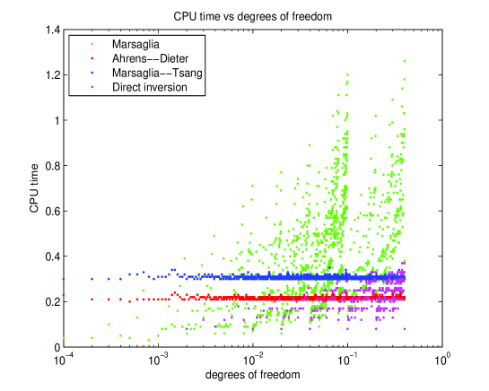
Figure 2: CPU time versus the number of degrees of freedom $\nu$ using the generalized Marsaglia, Ahrens–Dieter and Marsaglia–Tsang acceptance-rejection methods, as well as the direct inversion method. The ordinate shows the CPU time needed to generate $10^{5}$ samples, simultaneously for two sets of $\nu$ abscissa values given to three significant figures, namely $\nu=(1+m)\cdot 10^{-4}$ for $m=0,1,\ldots,1000$ and $\nu=0.101+m\cdot 10^{-3}$ for $m=0,1,\ldots,299$. We have omitted CPU times for the direct inversion method involving the fourth decimal place.

Remark 5

We could equivalently construct analogous Padé and polynomial approximations for the inverse $\chi^{2}_{\nu}$ distribution function. Indeed we could generate tables analogous to those in Appendix B for values of $\nu=0.4,0.2,0.1,0.04,0.02,0.01,\ldots$ and so forth. We chose to base our method on the generalized Gaussian distribution as: (i) we could use it to sample from both the generalized Gaussian and central chi-square distributions simultaneously and we thus afforded greater flexibility; (ii) we used the robust and highly effective Beasley–Springer–Moro method for the inverse Gaussian distribution as a starting point, and (iii) the behaviour of the generalized Gaussian distribution in the limit of large $q$—to a uniform $\text{U}(-1,1)$ distribution—was qualitatively and quantitatively appealing. However, suppose one knew beforehand that for a known fixed number of degrees of freedom $\nu$ many $\chi^{2}_{\nu}$ samples would be required. In such a scenario it may be worth expending preparation effort to generate Padé and polynomial approximations for that value of $\nu$, as one could then relatively efficiently sample using the inverse $\chi^{2}_{\nu}$ distribution function approximation.

Remark 6

Since the direct inversion method computes the inverse generalized Gaussian distribution function to very high accuracy (and in principle to machine error), it can be combined with variance-reducing Monte Carlo techniques, e.g. antithetic variates or conditional Monte Carlo where appropriate for the problem under consideration. A further advantage of direct inversion methods for the use of quasi-Monte Carlo simulation is that exactly one random input variable is required to generate one sample of the target distribution. See Chapter 2 in Glasserman Glass for a more detailed discussion.

3.4 Non-central chi-square sampling

We can generate non-central chi-square samples from central chi-square samples as follows. Following Johnson Jo1959 and Siegel Siegel any $\chi_{\nu}^{2}(\lambda)$ random variable can be decomposed as $\chi_{\nu}^{2}(\lambda)\sim\chi_{0}^{2}(\lambda)+\chi_{\nu}^{2}$. Here $\chi_{0}^{2}(\lambda)$ random variable can be generated by choosing a random variable $N$ from a Poisson distribution with mean $\lambda/2$, and then generating a central $\chi_{2N}^{2}$ sample. Also see Broadie and Kaya BK for more details. Hence we are left with the problem of how to sample from a $\chi_{2N}^{2}$ distribution—we use either of the two methods of the last section to sample from the $\chi_{\nu}^{2}$ distribution. The following algorithm produces a $\chi_{\nu}^{2}(\lambda)$ sample.

Algorithm 3 (Non-central chi-square samples)

1. Use Algorithm 1 or 2 to generate a $\chi_{\nu}^{2}$ random variable $Z$.

2. Generate a Poisson distributed random variable $N$ with mean $\lambda/2$.

3. Generate $N$ independent uniform $\text{U}(0,1)$ random variables $U_{1},\ldots,U_{N}$.

4. Compute $-2\bigl{(}\log(U_{1})+\cdots+\log(U_{N})\bigr{)}+Z\sim\chi_{\nu}^{2}(\lambda)$.

For small non-centrality $\lambda\leqslant 10$, we generate the Poisson random variable using the exact direct inversion method (inverse transform method) in Glasserman (Glass, , p. 128). (An alternative method for small non-centrality is the acceptance-rejection method found in Knuth (Knuth, , p. 137).) When the non-centrality parameter $\lambda>10$ we could use the Normal approximation from Fishman (Fish, , p. 212, paragraph 3): $\max\{0,\text{floor}(\lambda+1/2+\sqrt{\lambda}\,Y)\}$, where $Y$ is a standard Normal random variable. However we are endeavouring to retain accuracy as far as possible and prefer to avoid such approximations. There are several other notable methods for generating Poisson random variables in this parameter regime, in particular that of Ahrens and Dieter AD and the PRUA^∗ method found in Fishman (Fish, , p. 214); but these are acceptance-rejection methods.

Large non-centrality $\lambda>10$ is relevant to our applications to the Heston model: the Poisson mean is inversely proportional to the discretization stepsize, which is required to be small when for example one wishes to price path-dependent derivatives. We thus propose the following approach to chi-square sampling when the non-centrality parameter $\lambda$ is large, say larger than a critical value $\bar{\lambda}$, modifying Algorithm 3 as follows. The Poisson variable $N$ can be written as a sum of two independent Poisson random variables $\bar{N}$ and $P$ with mean $\bar{\lambda}/2$ and mean $\lambda/2-\bar{\lambda}/2$, respectively. The chi-square distribution can be represented as

$$\chi^{2}_{\nu}(\lambda)\sim\chi_{\nu+2N}^{2}\sim\chi_{\nu+2\bar{N}+2P}^{2}\sim\chi^{2}_{\nu+2\bar{N}}(\lambda-\bar{\lambda}).$$

We sample $\bar{N}$ from the Poisson distribution with parameter $\bar{\lambda}/2$ using the direct inversion method in Glasserman (Glass, , p. 128) (mentioned above for small non-centrality). If $\bar{N}\not=0$, then the $\chi^{2}_{\nu+2\bar{N}}(\lambda-\bar{\lambda})$ variable can be represented as a sum of a $\chi^{2}_{\nu}$ variable and an independent $\chi^{2}_{2\bar{N}}(\lambda-\bar{\lambda})$ variable $\chi^{2}_{\nu+2\bar{N}}(\lambda-\bar{\lambda})\sim\chi^{2}_{\nu}+\chi^{2}_{2\bar{N}}(\lambda-\bar{\lambda})$. A sample from this distribution can be generated efficiently by sampling $\bar{N}-1$ independent uniform $\text{U}(0,1)$ random variables, say $U_{1},\ldots,U_{\bar{N}-1}$, two independent standard normal random variables, say $V_{1}$ and $V_{2}$, and an independent $\chi_{\nu}^{2}$ random variable, say $Z$, using Algorithm 1. Then $-2(\log U_{1}+\cdots+\log U_{\bar{N}-1})+V_{1}^{2}+\bigl{(}V_{2}+\sqrt{\lambda-\bar{\lambda}}\bigr{)}^{2}+Z\sim\chi_{\nu+2\bar{N}}(\lambda-\bar{\lambda})$. If $\bar{N}=0$, then we have to sample a $\chi^{2}_{\nu}(\lambda-\bar{\lambda})$ random variable, but now with a non-centrality parameter $\lambda-\bar{\lambda}<\lambda$. If $\lambda-\bar{\lambda}\leqslant\bar{\lambda}$, then the direct inversion method in Glasserman (Glass, , p. 128) is an efficient method to sample from this distribution. If $\lambda-\bar{\lambda}$ is larger than $\bar{\lambda}$, then we repeat this process until the sample of the Poisson random variable with mean $\bar{\lambda}$ returns a non-zero value or until the non-centrality parameter is smaller than $\bar{\lambda}$, whichever comes first. To summarize, the algorithm is as follows.

Algorithm 4 (Chi-square samples for large non-centrality parameter)

1. If $\lambda>\bar{\lambda}$, generate a Poisson random variable $\bar{N}$ with mean $\bar{\lambda}/2$ using direct inversion or the method in Knuth.

2. 1. If $\bar{N}\not=0$

      1. generate $\bar{N}-1$ independent uniform $\text{U}(0,1)$ random variables, say $U_{1},\ldots$, $U_{\bar{N}-1}$, two independent standard normal random variables, say $V_{1}$ and $V_{2}$, and use Algorithm 1 to generate an independent $\chi^{2}_{\nu}$ random variable $Z$.

      2. Compute $-2(\log U_{1}+\cdots+\log U_{\bar{N}-1})+V_{1}^{2}+\bigl{(}V_{2}+\sqrt{\lambda-\bar{\lambda}}\bigr{)}^{2}+Z\sim\chi_{\nu}^{2}(\lambda)$.

   2. If $\bar{N}=0$, set $\lambda\leftarrow\lambda-\bar{\lambda}$.

      1. If $\lambda>\bar{\lambda}$, repeat from Step 1.

      2. If $\lambda\leqslant\bar{\lambda}$, use Algorithm 3 to generate an independent $\chi^{2}_{\nu}(\lambda)$ random variable.

Algorithm 4 provides an exact method to sample a $\chi_{\nu}^{2}(\lambda)$ random variable for a large non-centrality parameter. Note that $P\{\bar{N}\not=0\}=1-\exp(-\bar{\lambda}/2)$. The expected number of iterations to generate a chi-square sample is thus the minimum of $1/\bigl{(}1-\exp(-\bar{\lambda}/2)\bigr{)}$ and $\lfloor\lambda/\bar{\lambda}\rfloor$. However more importantly, note that the number of steps is bounded above by $\lfloor\lambda/\bar{\lambda}\rfloor$. In our applications, we set $\bar{\lambda}=20$. Thus the probability of performing Step 2(b) in Algorithm 4 is $P\{\bar{N}=0\}\approx 10^{-5}$, the probability of repeating Step 2(b) is of order $10^{-9}$. The probability of repeating Step 2(b) once more is of order $10^{-13}$. In most applications this can be considered negligibly small. Thus practically, Algorithm 4 can be stopped after a maximum of 2 iterations (beyond that a positive value could by arbitrarily assigned if required). Alternatively, we could enforce an upper bound on the total number of random variables required here, by using the Andersen–Patnaik matched normal squared approximation for non-centrality values $\lambda$ that are very large, i.e. large enough so as not to compromise the accuracy of the direct inversion method we have carried thus far.

Remark 7

When the number of degrees of freedom $\nu$ is one or greater, the decomposition $\chi_{\nu}^{2}(\lambda)\sim\chi_{1}^{2}(\lambda)+\chi_{\nu-1}^{2}$ radically simplifies the non-central chi-square simulation process. A $\chi_{1}^{2}(\lambda)$ random variable is straightforwardly generated by squaring an appropriately mean-shifted standard Normal random variable. If $\nu-1<1$ then a central $\chi_{\nu-1}^{2}$ random variable can be generated using the methods described above. Whilst if $\nu-1\geqslant 1$, then we can decompose $\chi_{\nu-1}^{2}\sim\chi_{\lfloor\nu-1\rfloor}^{2}+\chi_{\nu-1-\lfloor\nu-1\rfloor}^{2}$. The component involving the integer part of $\nu-1$, i.e. $\lfloor\nu-1\rfloor$, can be simulated by taking the sum of the logarithms of $\lfloor\nu-1\rfloor$ uniform random variables (by analogy with Step 4 in the Algorithm 3 above). The component involving the remaining fractional degrees of freedom $\nu-1-\lfloor\nu-1\rfloor$ can again be simulated using the methods described above.

4 Application: the Cox-Ingersoll-Ross process and Heston model

We illustrate the accuracy of our new methods for chi-square sampling of the CIR process applied to the Heston model.

4.1 The CIR process

The mean-reverting square-root process or Cox-Ingersoll–Ross (CIR) process was first used in a financial context by Cox, Ingersoll and Ross CIR to model the short rate of interest and has been applied in numerous financial applications since. It can be expressed in the form

$$\mathrm{d}V_{t}= \;\kappa(\theta-V_{t})\,\mathrm{d}t+\varepsilon\sqrt{V_{t}}\,\mathrm{d}W^{1}_{t},$$

where $W^{1}$ is a Wiener process and $\kappa$, $\theta$ and $\varepsilon$ are positive constants. It is a mean-reverting process with mean $\theta$, rate of convergence $\kappa$ and square root diffusion scaled by $\varepsilon$. By the Yamada condition this model has a unique strong solution. Interestingly, though the explicit form of the solution as a function of the driving Wiener process $W^{1}$ is not known, its transition probability is explicitly given as a scaled non-central chi-square distribution. We define the degrees of freedom for this process to be $\nu\coloneqq 4\kappa\theta/\varepsilon^{2}$. When $\nu\in\mathbb{N}$ the process $V_{t}$ can be reconstructed from the sum of squares of $\nu$ Ornstein–Uhlenbeck processes; hence the label of degrees of freedom. When $\nu<2$ the zero boundary is attracting and attainable, while when $\nu\geqslant 2$, the zero boundary is non-attracting. In particular, the CIR process is non-negative. These properties are immediate from the Feller boundary criteria, see Feller Feller . These are based on inverting the associated stationary elliptic Fokker–Planck operator, with boundary conditions, and can be found for example in Karlin and Taylor KT .

Here we focus on the challenge of $\nu<2$ and in particular cases when $\nu\ll\,1$. Importantly, though the zero boundary is attracting and attainable, it is strongly reflecting—if the process reaches zero it leaves it immediately and bounces back into the positive domain—see Revuz and Yor (RY, , p. 412). We detailed in the introduction how this case is a major obstacle, particularly for direct discretization methods. A comprehensive account of direct discretization methods can be found in Lord, Koekkoek and Van Dijk LKVD . The full truncation method proposed by Lord, Koekkoek and Van Dijk allows the variance process to be negative over successive timesteps—when the variance evolves deterministically with an upward drift of $\kappa\theta$ and the volatility of the price process is taken to be zero. Andersen An and Haastrecht and Pelsser HP complete thorough comparisons with full truncation method of Lord, Koekkoek and Van Dijk.

The method we propose follows the lead of Broadie and Kaya BK and is based on simulating the known transition probability density for the Cox–Ingersoll–Ross process. We quote the following form for this transition density, that can be found in Cox, Ingersoll and Ross CIR , from a proposition in Andersen An .

Proposition 1

Let $F_{\chi_{\nu}^{2}(\lambda)}(z)$ be the cumulative distribution function for the non-central chi-squared distribution with $\nu$ degrees of freedom and non-centrality parameter $\lambda$:

$$F_{\chi_{\nu}^{2}(\lambda)}(z)=\frac{\exp(-\lambda/2)}{2^{\nu/2}}\sum_{j=0}^{\infty}\frac{(\lambda/2)^{j}}{j!2^{j}\Gamma(\nu/2+j)}\int_{0}^{z}\xi^{\nu/2+j-1}\exp(-\xi/2)\,\mathrm{d}\xi.$$

Set $\nu\coloneqq 4\kappa\theta/\varepsilon^{2}$ and define $\eta(h)\coloneqq 4\kappa\,\exp(-\kappa h)/\varepsilon^{2}\bigl{(}1-\exp(-\kappa h)\bigr{)}$, where $h=t_{n+1}-t_{n}$ for distinct times $t_{n+1}>t_{n}$. Set $\lambda\coloneqq V_{t_{n}}\cdot\eta(h)$. Then conditional on $V_{t_{n}}$, $V_{t_{n+1}}$ is distributed as $\exp(-\kappa h)/\eta(h)$ times a non-central chi-squared distribution with $\nu$ degrees of freedom and and non-centrality parameter $\lambda$, i.e.

$$\mathbb{P}\bigl{(}V_{t_{n+1}}<x~{}\big{|}~{}V_{t_{n}}\bigr{)}=F_{\chi_{\nu}^{2}(\lambda)}\bigl{(}x\cdot\eta(h)/\exp(-\kappa h)\bigr{)}.$$

Hence for Cox–Ingersoll–Ross sampling from timestep $t_{n}$ to $t_{n+1}$, we set $\lambda=V_{t_{n}}\cdot\eta(h)$ and compute/approximate $V_{t_{n+1}}=\chi_{\nu}^{2}(\lambda)\cdot\exp(-\kappa h)/\eta(h)$.

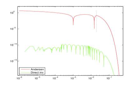
Figure 3: The absolute error in the direct inversion and Andersen approximations of the inverse chi-square $\chi_{\nu}^{2}$ distribution function for $\nu=0.02$. To the right of the vertical dotted line the Andersen approximation is identically zero and the curve shown represents the absolute difference between zero and the exact inverse distribution function.

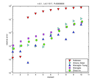
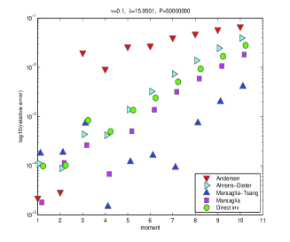
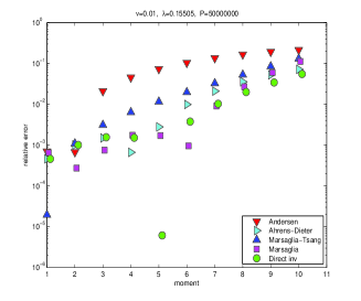
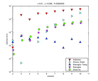
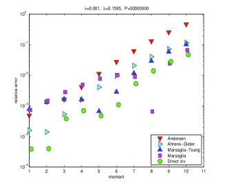
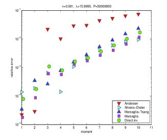
Figure 4: The relative error in the first through tenth moments of the non-central chi-square sampling methods shown. The six panels correspond to the three values of the degrees of freedom $\nu=0.1,0.01,0.001$ (top to bottom), and the values for the non-centrality $\lambda=0.11517,15.9501,0.15505,15.995,0.1595,15.9995$ (left to right, then top to bottom). The number of samples used in each case is $5\times 10^{7}$.

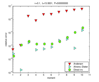
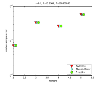
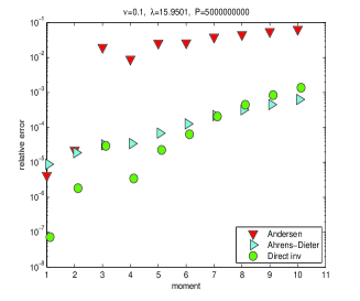
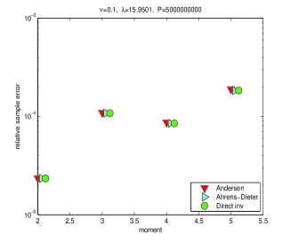
Figure 5: The left panels show the relative error in the first through tenth moments of the non-central chi-square sampling methods shown, for the case $\nu=0.1$, $\lambda=15.9501$ (corresponding to the upper right panel of Figure 4). In the top left panel we used $5\times 10^{8}$ samples, while in the lower left panel we used $5\times 10^{9}$ samples. The panels on the right show the corresponding relative sample errors for the second through fifth moments.

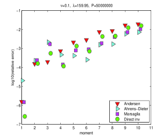
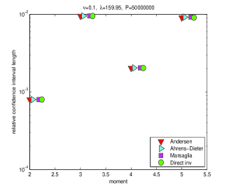
Figure 6: The left panels show the relative error in the first through tenth moments of the non-central chi-square sampling methods shown, for the case $\nu=0.1$, $\lambda=159.95$. We used $5\times 10^{7}$ samples. The panel on the right shows the corresponding relative sample errors for the second through fifth moments.

We illustrate in Figures 3, 4, 5 and 6 the performance in terms of accuracy of our direct inversion and generalized Marsaglia methods for a representative set of different parameter values for $\nu$ and $\lambda$. In Figure 3 the absolute error in the inverse distribution function for the direct inversion method compared with the leading approximation method of Andersen (more on this presently) is shown in the case of the central chi-square distribution with $\nu=0.02$ degrees of freedom. In Figure 4 the relative errors in the first ten sample central moments are displayed for simulating the non-central chi-square distribution using our methods. As comparison methods we chose Andersen’s approximation method, whose underlying parameters are fixed to match the first two central moments, and the exact acceptance-rejection methods of Ahrens–Dieter and Marsaglia–Tsang. The six panels shown therein correspond to the three values of the degrees of freedom $\nu=0.1,0.01,0.001$ (top to bottom), and the values for the non-centrality $\lambda=0.11517,15.9501,0.15505,15.995,0.1595,15.9995$ (left to right, then top to bottom). The number of samples used in each case was $5\times 10^{7}$. We observe that the relative errors in all three exact acceptance-rejection methods as well as the direct inversion method achieve the same high accuracy in all ten moments across all the parameter values. Indeed their accuracy is essentially limited by the Monte Carlo error which scales as the reciprocal of the square root of the sample size. Indeed to confirm this, we see in Figure 5 how their relative errors and relative sample errors decrease when the sample size is increased by a factor of $10$ and then $10^{2}$. Any variation in the relative errors between these four methods across all the plots in Figures 4 and 5 are within the corresponding sample errors. For the Andersen approximation method, we note that in the top left panel and all three right-hand panels in Figure 4, that the first two moments are indeed matched, while the accuracy in all the other moments is larger by several orders of magnitude. Further we observe in Figure 5 that the error in this approximation is invariant to increasing the sample size, thus exhibiting the bias in this method.

However we note in the two lower left panels in Figure 4 that as the number of degrees of freedom $\nu$ is decreased for small non-centrality, the performance of Andersen’s approximation improves and indeed matches that of the other methods in the case $\nu=0.001$ and $\lambda=0.1595$. This can be heuristically explained as follows. For small non-centrality, the Andersen approximation uses a weighted density function approximation given by $p\,\delta(0)+(1-p)\,\beta\exp(-\beta x)$, where the parameter $p=(s^{2}-m^{2})/(s^{2}+m^{2})$ characterizes the distribution between a mass density at the origin and a decaying exponential approximation scaled by the parameter $\beta=(1-p)/m$. Here $m$ and $s^{2}$ represent the sample mean and variance, respectively, and this weighted approximation is invoked when $s^{2}/m^{2}>1.5$. In Figure 4 to decrease $\nu$, we decreased $\kappa$; and note that we set $V(0)=\theta$, $\varepsilon=1$ and $h=1$. A straightforward calculation using the explicit values for $m$ and $s^{2}$ given in Andersen An , reveals that $s^{2}/m^{2}\sim 1/2\theta$ and thus $p\sim(1-2\theta)/(1+2\theta)$ for $\kappa\ll 1$. For small $\theta$, we see $p\to 1^{-}$. Note that $\theta=0.04$ in Figure 4. Since for small non-centrality the non-central chi-square distribution approaches the central chi-square distribution, and then for small degrees of freedom the central-square distribution shifts to concentrate high probability of occurrence to the origin where there is an integrable singularity, that the Andersen approximation shifts more weight to the point mass at the origin in this limit naturally shadows this phenomenon. Thus in this limit we might expect the Andersen approximation to perform better, as indicated in Figure 4.

The opposite extreme of the parameter space to this last case is that of very large non-centrality. We show in Figure 6 the the relative errors in the first ten sample central moments for the case when $\nu=0.1$ and $\lambda=159.95$. We see that all the methods perform roughly equally well in terms of accuracy across all the moments (we have not plotted the Marsaglia–Tsang case as this is in practice for the parameter regime $\nu<1$ of interest here slightly slower than the Ahrens–Dieter method as we discuss below, though this may not be the case for parameter values $\nu>1$). In particular the Andersen method performs equally well. This is not too surprising. It reflects the fact that for large centrality the Andersen method utilizes an observation by Patnaik Patnaik that a very effective approximation to the non-central chi-square distribution function is generated by the square of a matched normal random variable.

The improved accuracy requires a higher computational effort. In Table 1 we list the CPU times for each method relative to the CPU times of the Andersen method for each of the cases considered in Figures 4 and 6. For all the cases considered in Figure 4 the generalized Marsaglia and direct inversion methods require on average 1.41 and 1.46 times respectively more effort. The methods of Marsaglia–Tsang and Ahrens–Dieter are on average 2.8 and 2.55 times respectively slower (and thus hereafter we use the method of Ahrens–Dieter in preference for comparison). For the case in Figure 6 the generalized Marsaglia, direct inversion and Ahrens–Dieter methods require 5.25, 5.90 and 6.69 times respectively more effort. This is because for high non-centrality more effort is required to sum the larger number (a Poisson random variable with mean $\lambda/2$) of exponential random variables that are used to simulate the non-central component $\chi^{2}_{0}(\lambda)$ of the non-central $\chi_{\nu}^{2}(\lambda)$ random variable.

To be exhausting comprehensive, we also calculated relative CPU times when $\nu=0.777$ and $\lambda=15.6164$. This parameter value belongs to the computationally most expensive parameter cases for the direct inversion method. This due to the unfavourable decomposition of $\nu=0.777$ in our fractional basis $1/5,\,1/10,\,1/20,\,1/50,\,\ldots$, and the requirement to add powers of multiple generalized Gaussian variables, see Section 3.2. This could be alleviated by using a finer decomposition. As expected the Ahrens–Dieter method performance was unaffected (2.6803) while the direct inversion method was slower (3.1916). We emphasize that all our calculations were performed using compiled Matlab code. We endeavoured to optimize the performance of all the methods, for example using the Beasley–Springer–Moro methods for the Gaussian inversion required in the method of Andersen, and so forth.

$(\nu,\lambda)$	Marsaglia–Tsang	Ahrens–Dieter	Gen. Marsaglia	Direct inv.
$(0.1,0.11517)$	2.7855	2.5689	1.4479	1.3718
$(0.1,15.9501)$	2.8185	2.5683	1.6986	1.6135
$(0.01,0.1595)$	2.7953	2.5665	1.2207	1.4044
$(0.01,15.9995)$	2.8137	2.5554	1.4813	1.5990
$(0.001,0.1595)$	2.8300	2.5451	1.1640	1.3635
$(0.001,15.9995)$	2.7525	2.5326	1.3472	1.4918
$(0.1,159.95)$	$\cdots$	6.6921	5.2517	5.9027

Table 1: CPU times relative to the Andersen method to compute the moments in Figures 4 and 6 for the methods and parameters shown.

4.2 The Heston Model

The CIR process is a main ingredient in the Heston model (Heston H ). The Heston model is a two-factor model, in which one component $S$ describes the evolution of a financial variable such as a stock index or exchange rate, and the second component $V$ is a CIR process that describes the stochastic variance of its returns. It is given by

$$\mathrm{d}S_{t}= \;\mu S_{t}\,\mathrm{d}t+\sqrt{V_{t}}\,S_{t}\,\bigl{(}\rho\,\mathrm{d}W^{1}_{t}+\sqrt{1-\rho^{2}}\,\mathrm{d}W^{2}_{t}\bigr{)},$$

$$\mathrm{d}V_{t}= \;\kappa(\theta-V_{t})\,\mathrm{d}t+\varepsilon\sqrt{V_{t}}\,\mathrm{d}W^{1}_{t},$$

where $W^{1}_{t}$ and $W^{2}_{t}$ are independent scalar Wiener processes. The parameters $\mu$, $\kappa$, $\theta$ and $\varepsilon$ are all positive and $\rho\in(-1,1)$. In the context of option pricing, a pricing measure must be specified. We assume here that the dynamics of $S$ and $V$ as specified above are given under the pricing measure. For a discussion and derivation of various equivalent martingale measures in the Heston model see for example Hobson Ho . As noted above, the variance $V$ is non-negative, and the stock price $S$, as a pure exponential process, is positive. Without loss of generality we suppose $\mu=0$.

To estimate the asset price we follow the lead of Broadie and Kaya BK and Andersen An (also see Willard Willard and Romano and Touzi RT ). In the following proposition we assume we have simulated $V_{t_{n+1}}$ from $V_{t_{n}}$ exactly—for example using the non-central chi-square simulation scheme based on the generalized Marsaglia approach.

Proposition 2

Across the time step $[t_{n},t_{n+1}]$, assume $V_{t_{n}}$ and $V_{t_{n+1}}$ are given. Then set $K_{1}=h(\kappa\rho/{\varepsilon}-1/2)/2-\rho/{\varepsilon}$, $K_{2}=h(\kappa\rho/{\varepsilon}-1/2)/2+\rho/{\varepsilon}$, $K_{3}=h(1-\rho^{2})/2$, $s=K_{2}+K_{3}/2$, $\hat{s}=s\cdot\exp(-\kappa h)/\eta(h)$ and for $\hat{s}<1/2$,

$$K_{0}^{\ast}=-\frac{\lambda\hat{s}}{1-2\hat{s}}+(\nu/2)\cdot\ln(1-2\hat{s})-(K_{1}+K_{3}/2)V_{t_{n}}.$$

Then the approximate price process computed as follows is a martingale:

$$S_{t_{n+1}}=S_{t_{n}}\exp\Bigl{(}K_{0}^{\ast}+K_{1}V_{t_{n}}+K_{2}V_{t_{n+1}}+\sqrt{K_{3}(V_{t_{n}}+V_{t_{n+1}})}\cdot Z\Bigr{)},$$

where $Z\sim\mathrm{N}(0,1)$.

Proof

With $V_{t_{n}}$ and $V_{t_{n+1}}$ as given, conditioned on the time integrated variance across $[t_{n},t_{n+1}]$, we know that $\ln S_{t_{n+1}}-\ln S_{t_{n}}$ is Normally distributed. As suggested by Andersen, we approximate the time integrated variance across $[t_{n},t_{n+1}]$ by the trapezoidal rule. Exponentiating we arrive at the scheme from Andersen (An, , p. 21):

$$S_{t_{n+1}}=S_{t_{n}}\exp\Bigl{(}K_{0}+K_{1}V_{t_{n}}+K_{2}V_{t_{n+1}}+\sqrt{K_{3}(V_{t_{n}}+V_{t_{n+1}})}\cdot Z\Bigr{)},$$

where $Z\sim\mathrm{N}(0,1)$ and $K_{0}=-h\rho\kappa\theta/{\varepsilon}$. Then as suggested in Proposition 7 of Andersen (An, , p. 21), if we set $M\coloneqq\mathbb{E}\bigl{[}\exp(sV_{t_{n+1}})|V_{t_{n}}\bigr{]}$ and $K_{0}^{\ast}\coloneqq-\ln M-(K_{1}+K_{3}/2)V_{t_{n}}$, and replace $K_{0}$ by $K_{0}^{\ast}$ in the scheme for $S_{t_{n+1}}$ above, then $\mathbb{E}[S_{t_{n+1}}|S_{t_{n}}]=S_{t_{n}}$. Hence our task is to compute $M$. Since we simulate $V_{t_{n+1}}$ exactly we know $M=\mathbb{E}\bigl{[}\exp(\hat{s}\cdot z)|V_{t_{n}}\bigr{]}$, where $z\sim\chi_{\nu}^{2}(\lambda)$, with $\nu$ and $\lambda$ defined for the Heston model. Hence provided $\hat{s}<1/2$ we have $M=\exp\bigl{(}\lambda\hat{s}/(1-2\hat{s})\bigr{)}/(1-2\hat{s})^{\nu/2}$, giving the result. ∎

Remark 8

The requirement $\hat{s}<1/2$ translates to a mild restriction on the stepsize $h$, which in practice is not a problem (see Andersen (An, , p. 24)).

We test all the methods we have considered, Andersen, Ahrens–Dieter, generalized Marsaglia and direct inversion for pricing five practical and challenging options. We use Andersen’s test cases I–III for pricing long-dated European call options (maturing at time $T$). Andersen describes case I as typical for FX markets, case II as typical for long-dated interest rate markets and case III as possible in equity option markets. We also considered Smith’s test case for an Asian option (see Smith Smith and Haastrecht and Pelsser HP ) and Lord, Koekkoek and Van Dijk’s test case for a digital double no touch barrier option. The parameter values for all five cases are shown in Table 2. Note that in case III, we have assumed the risk-free rate of interest $r=0.05$, as in Haastrecht and Pelsser HP . Let the exact option price at maturity be $C$. The error of the approximation is $E=C-\hat{C}$, where $\hat{C}$ is the sample average of the simulated option payout at maturity. In our examples, we use a sample size of $10^{6}$ (except for the barrier option case). The performance of the method of Haastrecht and Pelsser HP is similar to Andersen’s; the reader interested in the actual comparisons is referred to their paper. In Table 3 we show, for the test cases I–III, the relative CPU times to required to compute the option prices compared to Andersen’s method. The errors at three different strikes $100,140,60$, which are dominated by the trapezoidal rule approximation in the price process, are all comparable to Andersen’s method and so we omit them. We did not implement any postprocessing such as variance reduction here. We see from Table 3 that for these plain vanilla option cases, Andersen’s method is in fact the slowest.

We show in Table 4 the simulation results for the Asian option with yearly fixings, with very similar conclusions in terms of accuracy. The generalized Marsaglia and direct inverse methods are now almost two times slower than Andersen’s method in this case due to the slightly unfavourable form of the degrees of freedom $\nu=0.904$ (in these two cases we rounded off the exact degrees of freedom $\nu=0.9035$). However the accuracy they deliver for the variance process far outweighs their relative speed.

We also apply the four methods to pricing a digital double no touch barrier option—such an option pays one unit of currency if neither barrier is touched and zero if one is. We monitor at each timestep to determine if either of the barriers had been crossed. Indeed, we show in Table 5 our simulation results. In terms of accuracy for the stepsizes shown, all the methods perform equally well. In terms of CPU time, all the methods are faster or roughly the same speed as Andersen’s method, though the form of the number of degrees of freedom in this case $\nu=0.08$ favours the generalized Marsaglia and direct inversion methods. Note that small timesteps are considered in this test case. This means that the non-centrality parameter $\lambda$ can be large for some time intervals; in which case we use Algorithm 4 to generate chi-square samples.

Parameters	Case I	Case II	Case III	Case Asian	Case DDNT
${\varepsilon}$	1.0	0.9	1.0	0.5196	1.0
$\kappa$	0.5	0.3	1.0	1.0407	0.5
$\rho$	-0.9	-0.5	-0.3	-0.6747	0.0
$T$	10	15	5	4	1
$\theta$	0.04	0.04	0.09	0.0586	0.04
$S(0)$	100	100	100	100	100
$V(0)$	0.04	0.04	0.09	0.0194	0.04
$r$	0.0	0.0	0.05	0.0	0.0

Table 2: Cases I—III are from Andersen, while Case Asian is from Smith and Case DDNT (digital double no touch barrier option) is from Lord, Koekkoek and Van Dijk. Here $r$ is the risk-free rate of interest.

Case	Ahrens–Dieter	Marsaglia	Direct inv.
I	0.62	0.27	0.26
II	0.59	0.80	0.55
III	0.57	1.04	0.39

Table 3: Cases I—III from Andersen: we show the relative CPU times (to the method of Andersen) for pricing the options concerned using $10^{6}$ paths. The values shown are averaged across stepsizes $1/4$, $1/8$, $1/16$ and $1/32$—there was hardly any variation for different stepsizes.

Stepsize	Andersen	Ahrens–Dieter	Marsaglia	Direct inv.
1/4	[-0.0113,1]	[-0.0090,1.41]	[-0.0287,2.20]	[0.0719,2.19]
1/8	[-0.0166,1]	[-0.0151,1.30]	[-0.0073,2.02]	[0.0519,1.99]
1/16	[-0.0175,1]	[-0.0082,1.26]	[0.0240,1.95]	[0.0628,1.90]
1/32	[-0.0287,1]	[-0.0376,1.24]	[-0.0393,1.90]	[0.0604,1.86]

Table 4: Case Asian from Smith: Estimated error using $10^{6}$ paths for at the money Asian option (strike $100$) with yearly fixings. In each case the two-tuple shown is the estimated error and relative CPU time required to compute the option price. In all cases the sample standard deviation was $0.014$. All estimated errors are not statistically significant at the level of three sample standard deviations.

$h$	Andersen	Ahrens–Dieter	Marsaglia	Direct inv.
1/250	[0.5266,2.00,1]	[0.5300,0.63,0.76]	[0.5238,2.00,0.81]	[0.5300,2.00,0.96]
1/500	[0.5205,1.00,1]	[0.5208,0.32,0.77]	[0.5191,1.00,0.83]	[0.5194,1.00,0.99]
1/1000	[0.5154,0.50,1]	[0.5150,0.16,0.78]	[0.5147,0.50,0.87]	[0.5148,0.50,1.03]
1/2000	[0.5111,0.25,1]	[0.5105,0.08,0.86]	[0.5109,0.25,0.87]	[0.5108,0.25,1.02]

Table 5: Case DDNT from Lord, Koekkoek and Van Dijk: Estimated option price for the digital double no touch barrier option, using $1/h^{2}$ paths where $h$ is the stepsize. The barriers are 110 and 90. In each case the triple shown is the estimated price, the sample standard deviation (inflated by $10^{3}$) and relative CPU time required to compute the option price.

Remark 9

Note that for cases I–III we could improve the efficiency of the algorithm we have implemented as follows (and with mild modification to the Asian option with yearly fixings as well). We decompose $\int{V_{\tau}}\,\mathrm{d}\tau$ on $[0,T]$ into subintervals $[t_{n},t_{n+1}]$, use a simple quadrature to approximate $\int{V_{\tau}}\,\mathrm{d}\tau$ on these subintervals much like Andersen, and simulate the transition densities required using the generalized Marsaglia method. We then only exponentiate at the final time $T$ to generate an approximation for $S_{T}$ (since we do not compute the price process at each timestep, this will be more efficient). However, one advantage of the approach we have taken in this paper for simulating the price process based on the method proposed by Andersen, is that it is more flexible. For example, it allows us to consider pricing path-dependent options.

Remark 10

Glasserman and Kim GK have recently introduced a novel method for simulating the time integrated variance process in the Heston model (also see Chan and Joshi CJ ). As we can see from our analysis above, to compute the price process at the end-time $T$, we in essence need to sample from the distribution for $\int{V_{\tau}}\,\mathrm{d}\tau$ on the interval $[0,T]$. The transition density for this integral process over the whole interval $[0,T]$, given $V_{0}$ and $V_{T}$, is well known and given in Pitman and Yor PY . Its Laplace or Fourier transform has a closed form. Broadie and Kaya BK use Fourier inversion techniques to sample from this transition density for $\int{V_{\tau}}\,\mathrm{d}\tau$. Glasserman and Kim instead separate the Laplace transform of this transition density into constituent factors, each of which can be interpreted as the Laplace transforms of probability densities, samples of which can be generated by series of particular gamma random variables. The advantage of this method is that $\int{V_{\tau}}\,\mathrm{d}\tau$ is simulated directly on the interval $[0,T]$. Glasserman and Kim have demonstrated that this is an efficient alternative to the quadrature approximation of the time integrated variance suggested by Andersen, if one is interested in the pricing non-path-dependent derivatives, which does not require the simulation of any intermediate values of the asset process $S$. They also note that when pricing path-dependent options, quadrature approximation of the time integral of the variance process will be more efficient (see end of their Section 5).

5 Concluding remarks

We have introduced two new methods for sampling the CIR non-central chi-square process. The first is the generalized Marsaglia method which is an exact acceptance-rejection method. The second is a direct inversion method based on the Beasley–Springer–Moro method which delivers very high accuracy, and which in principle can be extended to machine accuracy (double precision). This method has the advantage of being amenable to implementation and simulation using quasi-Monte Carlo sequences as well as for sensitivity analysis. Both methods are easy to implement and flexible as the CIR process, which serves as a fundamental building block in many financial models, can be immediately simulated for any value of degrees of freedom. We illustrated their accuracy and their efficiency for an extensive range of parameter values. The efficiency performance of both methods are similar and compare well with other leading chi-square sampling methods. We illustrated the use of our new methods for the simulation of the Heston model. In terms of simulating the Heston model the accuracy delivered for the variance process is somewhat overridden by the error associated with the trapezoidal rule approximation used in the price process simulation. We expect that if the new more accurate approximation method of Glasserman and Kim for the integrated variance process is used instead, the accuracy available for the variance process will become more prevalent. Lastly, another additional direction of interest would be to consider how to optimize both our methods for use in general processing units (GPUs); see for example Giles Giles who considers an efficient approximation of the inverse error function for GPU execution.

Appendix A Generalized Gaussian direct inversion algorithm

Here we have assumed $(3,4)$ Padé approximants in both the central and middle regions and a degree $10$ Chebychev approximant in the tail region. Adapting the algorithm to other degree approximants is straightforward. We assume $q$ is given and the parameters $\gamma_{q}$, $C_{q}$, $\Phi_{\pm}$, $\eta_{*}$, $k_{1}$ and $k_{2}$ defined in Section 2.2 have been calculated as well. In the algorithm below these parameters are: gamma_q, C_q, Phi_minus, Phi_plus, eta_star, k_1 and k_2. Further the coefficients $a_{0},a_{1},a_{2},a_{3},c_{0},c_{1},c_{2},c_{3}$ are stored as the vectors a and c with index starting at 1, so $a_{0}$ corresponds to a(1), $a_{1}$ to a(2), etc., whereas the coefficients $b_{1},b_{2},b_{3},b_{4},d_{1},d_{2},d_{3},d_{4}$ are stored as the vectors b and d with exact indexing correspondence. The coefficients $\hat{c}_{0},\ldots,\hat{c}_{10}$ are stored as the vector c_ hat with index running from 1 to 11. The input U is a $\text{U}(0,1)$ uniform random variable and the output X is a generalized Gaussian random variable.

Listing 1: Generalized Gaussian direct inversion

⬇

Y=(U-0.5)/gamma_q;

if (abs(Y)<(Phi_minus-0.5)/gamma_q)

R=Y^q;

X=Y*(((a(4)*R+a(3))*R+a(2))*R+a(1)) ...

/((((b(4)*R+b(3))*R+b(2))*R+b(1))*R+1.0);

else

R=1-U;

if (Y<0)

R=U;

end

if (abs(U-0.5)<Phi_plus-0.5)

R=-log(R)-eta_star;

X=(((c(4)*R+c(3))*R+c(2))*R+c(0)) ...

/((((d(4)*R+d(3))*R+d(2))*R+d(1))*R+1.0);

else

R=k_1*log(-log(R/C_q))+k_2;

D2=0;

D1=0;

for j=10:-1:1

D=2*R*D1-D2+c_hat(j+1);

D2=D1;

D1=D;

end

X=R*D1-D2+0.5*c_hat(1);

end

if (Y<0)

X=-X;

end

end

Appendix B Direct inversion coefficients

$q=10$
n	$a_{n}$	$c_{n}$	$n$	$\hat{c}_{n}$
0	0.999999999999651	1.060540481693800	0	2.622284617034058
1	-1.429881128897603	0.796155091482938	1	0.1449805130767122
2	0.601262815177118	0.206235219404016	2	0.003259370325482870
3	-0.068206095200774	0.020226513592948	3	-0.0003397434921419157
4		0.000479843137311	4	0.00007014928432054771
			5	-0.000003586305447050563
	$b_{n}$	$d_{n}$	6	-7.631531772738493$*10^{-7}$
1	-1.475335674435254	0.683564944492548	7	1.840112411709724$*10^{-7}$
2	0.651548639035629	0.161851250036749	8	-1.217436540241387$*10^{-8}$
3	-0.081616351333977	0.014123257065970	9	-2.007039183742053$*10^{-9}$
4	0.000391957158842	0.000270655354670	10	5.694689247537491$*10^{-10}$
	$\Phi_{-}$	$\Phi_{+}$		$\eta_{*}$
	0.954178994865017	0.998325461835062		4.254756463685820
	$k_{1}$	$k_{2}$
	1.015803736413048	-2.256872281479897
$q=100$
n	$a_{n}$	$c_{n}$	$n$	$\hat{c}_{n}$
0	0.999999999999675	1.006854352727258	0	2.053881658435666
1	-1.582783912975250	0.731099829867281	1	0.01034073560906051
2	0.745662878312873	0.195140887172246	2	-0.00002227561625609034
3	-0.097011209317889	0.021377534151187	3	-0.00002539481838124709
4		0.000693785524959	4	0.000005279864625853940
			5	-3.805077742014832$*10^{-7}$
	$b_{n}$	$d_{n}$	6	-3.298923929556226$*10^{-8}$
1	-1.587734408086399	0.720091560042297	7	1.114785567355588$*10^{-8}$
2	0.751669594595948	0.190684456942316	8	-9.757310866073955$*10^{-10}$
3	-0.098779495517049	0.020677157072949	9	-6.769928792613323$*10^{-11}$
4	0.000055151948082	0.000659853425082	10	2.803447160471445$*10^{-11}$
5		-0.000000097154009
	$\Phi_{-}$	$\Phi_{+}$		$\eta_{*}$
	0.996245001605534	0.999888263643581		6.788371878124332
	$k_{1}$	$k_{2}$
	1.130241473667677	-2.510876893558557
$q=1000$
n	$a_{n}$	$c_{n}$	$n$	$\hat{c}_{n}$
0	0.999999999996602	1.000692386269727	0	2.005202593715361
1	-2.214484997909744	0.641334743798204	1	0.0009445439483225688
2	1.455225242281931	0.146036839714129	2	-0.000003302159950131867
3	-0.270311067182453	0.012706381032885	3	-0.000002214168006581846
		0.000254873053744	4	4.226488352359718$*10^{-7}$
			5	-2.701556647692559$*10^{-8}$
	$b_{n}$	$d_{n}$	6	-2.660957832417678$*10^{-9}$
1	-2.214984498880292	0.640293981966015	7	7.589961583952764$*10^{-10}$
2	1.456144357614843	0.145674000937359	8	-5.604691330255176$*10^{-11}$
3	-0.270724201676657	0.012660105958367	9	-5.184165197371945$*10^{-12}$
4	0.000022976139411	0.000253400757973	10	1.626439890027763$*10^{-12}$
	$\Phi_{-}$	$\Phi_{+}$		$\eta_{*}$
	0.999632340672519	0.999989279922375		9.115135573141224
	$k_{1}$	$k_{2}$
	1.211390454015218	-2.630859238259484

$q=5$
n	$a_{n}$	$c_{n}$	$n$	$\hat{c}_{n}$
0	0.999999999999962	1.098560543273500	0	3.446913820849123
1	-1.288113131377250	1.076929115611482	1	0.4032831311503550
2	0.481578771462415	0.374009830584217	2	0.02171691866430493
3	-0.047325498551885	0.052979687032815	3	-0.0003693910171288154
4		0.002320423236613	4	0.0001643478336907373
			5	-9.968595138386470$*10^{-7}$
	$b_{n}$	$d_{n}$	6	-0.000002678275851276468
1	-1.371446464722253	0.826900637356423	7	4.340978214450863$*10^{-7}$
2	0.565562947138128	0.243236630017604	8	-8.359190851308088$*10^{-9}$
3	-0.067614258837771	0.028035297860946	9	-8.345847144867538$*10^{-9}$
4	0.000560269685859	0.000866824877085	10	1.501644408119446$*10^{-9}$
5		-0.000003203247416
	$\Phi_{-}$	$\Phi_{+}$		$\eta_{*}$
	0.888435024173769	0.994853658080896		3.327051730489134
	$k_{1}$	$k_{2}$
	0.9436583821081551	-2.053011104657458
$q=50$
n	$a_{n}$	$c_{n}$	$n$	$\hat{c}_{n}$
0	0.999999999999476	1.013549868031473	0	2.109911415053862
1	-1.564458809116706	0.667930936229205	1	0.02170729783674736
2	0.727524267692390	0.155499481214690	2	0.000005070046142588313
3	-0.093190467403288	0.013822381509740	3	-0.00005423065778776348
4		0.000286136307044	4	0.00001132985142947280
			5	-8.168939038096652$*10^{-7}$
	$b_{n}$	$d_{n}$	6	-7.483150884891461$*10^{-8}$
1	-1.574262730786144	0.646800829595665	7	2.519301860662225$*10^{-8}$
2	0.739293882226217	0.147982563681919	8	-2.231412272701264$*10^{-9}$
3	-0.096615964501066	0.012852173023820	9	-1.581249637852744$*10^{-10}$
4	0.000106012694153	0.000254893106908	10	6.651970666939820$*10^{-11}$
	$\Phi_{-}$	$\Phi_{+}$		$\eta_{*}$
	0.992313833379312	0.999766047505894		6.068592841104139
	$k_{1}$	$k_{2}$
	1.104377984691796	-2.464549291690036
$q=500$
n	$a_{n}$	$c_{n}$	$n$	$\hat{c}_{n}$
0	1.000000000001737	1.001383246165305	0	2.010495391375142
1	-1.391636943669522	0.643915677152308	1	0.001933087453438041
2	0.529242181140450	0.147299234948298	2	-0.000006861856172820585
3	-0.043796708347591	0.012900083582821	3	-0.000004593728077441438
4		0.000260965296708	4	9.054993169060948$*10^{-7}$
			5	-6.064260759136934$*10^{-8}$
	$b_{n}$	$d_{n}$	6	-5.622897885014598$*10^{-9}$
1	-1.392634947413242	0.641830834617498	7	1.709975585729971$*10^{-9}$
2	0.530257903665352	0.146569705446697	8	-1.346040760729119$*10^{-10}$
3	-0.044005529297217	0.012806476344300	9	-1.115867483028221$*10^{-11}$
4		0.000257963030654	10	3.854801783433290$*10^{-12}$
	$\Phi_{-}$	$\Phi_{+}$		$\eta_{*}$
	0.999262947245193	0.999978460704705		8.419292019151525
	$k_{1}$	$k_{2}$
	1.186173840297473	-2.595663671659387

$q=20$
n	$a_{n}$	$c_{n}$	$n$	$\hat{c}_{n}$
0	0.999999999999362	1.032613218276406	0	2.288521173202021
1	-1.511386771163247	0.713123517283527	1	0.06094747962391468
2	0.676248487105209	0.172466963210780	2	0.0004979897167054818
3	-0.082692565611279	0.015897412011461	3	-0.0001543431236869771
4		0.000346782310140	4	0.00003160495474050310
			5	-0.000002097939830730025
	$b_{n}$	$d_{n}$	6	-2.545431143318975$*10^{-7}$
1	-1.535196295102288	0.659013658465100	7	7.644348818405340$*10^{-8}$
2	0.703944802836950	0.152518516830577	8	-6.332863001383525$*10^{-9}$
3	-0.090485340265877	0.013264787335393	9	-5.895856800809525$*10^{-10}$
4	0.000235676079099	0.000260023340056	10	2.181280362294034$*10^{-10}$
	$\Phi_{-}$	$\Phi_{+}$		$\eta_{*}$
	0.979433650152057	0.999329809791150		5.073863838784834
	$k_{1}$	$k_{2}$
	1.062049352492145	-2.373877078913848
$q=200$
n	$a_{n}$	$c_{n}$	$n$	$\hat{c}_{n}$
0	0.999999999999818	1.003446599107830	0	2.026585952893378
1	-1.592059576219168	0.646500675620922	1	0.005000572651842971
2	0.754928347929758	0.147774949658364	2	-0.00001586472529618898
3	-0.098984011870256	0.012900041834309	3	-0.00001209785441132469
4		0.000259966165110	4	0.000002470674959854400
			5	-1.739180236341302$*10^{-7}$
	$b_{n}$	$d_{n}$	6	-1.521404951930557$*10^{-8}$
1	-1.594547138442268	0.641281532007261	7	4.971592453081240$*10^{-9}$
2	0.757962823762529	0.145949090224436	8	-4.195656728956311$*10^{-10}$
3	-0.099882437363767	0.012666874097162	9	-3.074520478566509$*10^{-11}$
4	0.000028130467837	0.000252543685829	10	1.193471454418927$*10^{-11}$
	$\Phi_{-}$	$\Phi_{+}$		$\eta_{*}$
	0.998144331394750	0.999945402061219		7.494926977014854
	$k_{1}$	$k_{2}$
	1.154337013616336	-2.549188505020307
$q=2000$
n	$a_{n}$	$c_{n}$	$n$	$\hat{c}_{n}$
0	0.999999999997019	1.000346383496690	0	2.002579775991956
1	-1.455537231516898	0.688914570824710	1	0.0004617142213663357
2	0.588358222689532	0.174806929040730	2	-0.000001526635305931853
3	-0.053434409210900	0.017594316937225	3	-0.000001066615247993659
4		0.000421430584942	4	1.965467095261218$*10^{-7}$
			5	-1.191943072817269$*10^{-8}$
	$b_{n}$	$d_{n}$	6	-1.255808491556965$*10^{-9}$
1	-1.455787106562329	0.688377683635393	7	3.345974182790842$*10^{-10}$
2	0.588628288218368	0.174601235888502	8	-2.298521347563630$*10^{-11}$
3	-0.053495358024573	0.017563762752719	9	-2.387233298590672$*10^{-12}$
4		0.000420251890153	10	6.789837048813090$*10^{-13}$
	$\Phi_{-}$	$\Phi_{+}$		$\eta_{*}$
	0.999816386904579	0.999994652315274		9.809631850391680
	$k_{1}$	$k_{2}$
	1.238207674406019	-2.667612981028375

References

- (1) J.H. Ahrens and U. Dieter, Computer generation of Poisson deviates from modified normal distributions, ACM Transactions on Mathematical Software, 8(2) (1982), pp. 163–179.
- (2) J.H. Ahrens and U. Dieter, Computer methods for sampling from gamma, beta, Poisson, and binomial distributions, Computing, 12 (1974), pp. 223–246.
- (3) A. Alfonsi, On the discretization schemes for the CIR (and Bessel squared) processes, Monte Carlo Methods and Applications, 11(4) (2005), pp. 355–384.
- (4) A. Alfonsi, High order discretization schemes for the CIR process: application to affine term structure and Heston models, Math. Comp., 79(269) (2010), pp. 209–237.
- (5) L. Andersen, Simple and efficient simulation of the Heston stochastic volatility model, Journal of Computational Finance, 11(3) (2008), pp. 1–42.
- (6) L.B.G. Andersen and V.V. Piterbarg, Moment explosions in stochastic volatility models, Finance and Stochastics, 11(1) (2007), pp. 29–50.
- (7) Beasley and Springer, The percentage points of the normal distribution, Applied Statistics, 26(1) (1977), pp. 118–121.
- (8) A. Berkaoui, M. Bossy and A. Diop, Euler scheme for SDEs with non-Lipschitz diffusion coefficient: strong convergence, ESAIM Probability and Statistics, 12 (2008), pp. 1–11.
- (9) P. Billingsley, Probability and measure, Wiley series in Probability and Mathematical Statistics, John Wiley & Sons, Inc., 1995.
- (10) J.M. Blair, C.A. Edwards and J.H. Johnson, Rational Chebyshev approximations for the inverse of the error function, Math. Comp. 30(136) (1976), pp. 827–830.
- (11) M. Bossy and A. Diop, An efficient discretization scheme for one dimensional SDEs with a diffusion coefficient function of the form , , INRIA Rapport de recherche n∘ 5396, 2007.
- (12) D. Brigo and K. Chourdakis, Counterparty risk for credit default swaps, International Journal of Theoretical and Applied Finance, 12(7) (2009), pp. 1007–1026.
- (13) M. Broadie and Ö. Kaya, Exact simulation of stochastic volatility and other affine jump diffusion processes, Operations Research, 54(2) (2006), pp. 217–231.
- (14) P. Carr and D.B. Madan, Option valuation using the fast Fourier transform, Journal of Computational Finance, 2(4) (1999), pp. 61–73.
- (15) G.D. Chalmers and D.J. Higham, First and second moment reversion for a discretized square root process with jumps, Preprint December 17, 2008.
- (16) J.H. Chan and M. Joshi, Fast and accurate long stepping simulation of the heston stochastic volatility model, SSRN preprint, 2010.
- (17) J.C. Cox, J.E. Ingersoll and S.A. Ross, A theory of the term structure of interest rates, Econometrica, 53(2) (1985), pp. 385–407.
- (18) G. Deelstra and F. Delbaen, Convergence of discretized stochastic (interest rate) processes with stochastic drift term, Appl. Stochastic Models Data Anal., 14 (1998), pp. 77–84.
- (19) S. Dereich, A. Neuenkirch and L. Szpruch, An Euler-type method for the strong approximation of the Cox-Ingersoll-Ross process, Proc R Soc A, 468 (2012), pp. 1105–1115, doi:10.1098/rspa.2011.0505.
- (20) D. Duffie and P. Glynn, Efficient Monte Carlo simulation of security prices, The Annals of Applied Probability, 5(4) (1995), pp. 897–905.
- (21) S. Dyrting, Evaluating the non-central chi-square distribution for the Cox–Ingersoll–Ross process, Computational economics, 24 (2004), pp. 35–50.
- (22) F. Fang and K. Oosterlee, Pricing early-exercise and discrete barrier options by Fourier-cosine series expansions, Numer. Math., 114 (2009), pp.27–62.
- (23) F. Fang and K. Oosterlee, A novel pricing method for European options based on Fourier-cosine series expansions, SIAM J. Sci. Comput., 30(2) (2008), pp. 826–848.
- (24) W. Feller, Two singular diffusion problems, Annals of Mathematics, 54 (1951), pp. 173–182.
- (25) G.S. Fishman, Monte Carlo: concepts, algorithms, and applications, Springer, 1995.
- (26) M. Giles, Approximating the erfinv function, Chapter 10 in GPU Computing Gems, Jade Edition, Editor-in-Chief: Wen-Mei W. Hwu, Morgan Kaufmann’s Applications of GPU Computing Series, 2012.
- (27) P. Glasserman, Monte Carlo methods in financial engineering, Applications of Mathematics, Stochastic Modelling and Applied Probability, 53, Springer, 2003.
- (28) P. Glasserman and K. Kim, Gamma expansion of the Heston stochastic volatility model, Finance Stoch., 15(2) (2011), pp. 267–296, DOI 10.1007/s00780-009-0115-y.
- (29) A.K. Gupta and D. Song, -norm spherical distribution, Journal of Statistical Planning and Inference, 60 (1997), pp. 241–260.
- (30) A. van Haastrecht and A. Pelsser, Efficient, almost exact simulation of the Heston stochastic volatility model, International Journal of Theoretical and Applied Finance, 13(1) (2010), pp. 1–43, DOI 10.1142/SO219024910005668.
- (31) T. Haentjens and K. in ’t Hout, ADI finite difference schemes for the Heston-Hull-White PDE, arXiv:1111.4087v1 (2012).
- (32) R. Harman and V. Lacko, On decompositional algorithms for uniform sampling from -spheres and -balls, Journal of Multivariate Analysis, 101 (2010), pp. 2297–2304.
- (33) S.L. Heston, A closed-form solution for options with stochastic volatility with applications to bond and currency options, Review of Financial Studies, 6(2) (1993), pp. 327–343.
- (34) D. Hobson, Stochastic volatility models, correlation, and the q-optimal measure, Mathematical Finance, 14 (2004), pp. 537-556.
- (35) D.J. Higham and X. Mao, Convergence of Monte–Carlo simulations involving the mean-reverting square root process, Journal of Computational Finance, 8 (2005), pp. 35–61.
- (36) D.J. Higham, X. Mao and A.M. Stuart, Strong Convergence of Numerical Methods for Nonlinear Stochastic Differential Equations, SIAM J. Num. Anal, 40 (2002), pp. 1041–1063.
- (37) K. In ’t Hout and S. Foulin ADI finite difference schemes for option pricing in the Heston model with correlation, International Journal of Numerical Analysis and Modeling, 7(2), pp. 303–320.
- (38) A. Jentzen, P.E. Kloeden and A. Neuenkirch, Pathwise approximation of stochastic differential equations on domains: Higher order convergence rates without global Lipschitz coefficients, Numerische Mathematik, 112(1) (2009), pp 41–64.
- (39) N.L. Johnson, On an extension of the connection between Poisson and distributions, Biometrika, 46 (3/4) (1959), pp. 352–363.
- (40) C. Joy, P.P. Boyle and K.S. Tan, Quasi-Monte Carlo methods in numerical finance, Management Science, 42(6) (1996), pp. 926–938.
- (41) C. Kahl, M. Günther and T. Roßberg, Structure preserving stochastic integration schemes in interest rate derivative modeling, Appl. Numer. Math., 58(3) (2008), pp. 284–295.
- (42) C. Kahl and P. Jäckel, Fast strong approximation Monte Carlo schemes for stochastic volatility models, Quant. Finance, 6(6) (2006), pp. 513–536.
- (43) C. Kahl and P. Jäckel, Not-so-complex logarithms in the Heston Model, Wilmott, September 2005, pp. 94–103.
- (44) C. Kahl and H. Schurz, Balanced Milstein methods for ordinary SDEs, Monte Carlo Methods Appl., 12(2) (2006), pp. 143–170.
- (45) S. Karlin and H.M. Taylor, A second course in stochastic processes, Academic Press, 1981.
- (46) D.E. Knuth, The art of computer programming, vol 2: Seminumerical algorithms, Addison-Wesley, Reading, Mass., Third edition, 1998.
- (47) V. Lacko and R. Harman, A conditional distribution approach to uniform sampling on spheres and balls in spaces, Metrika (2011), DOI: 10.1007/s00184-011-0360-x.
- (48) J. Liang and K.W. Ng, A method for generating uniformly scattered points on the -norm unit sphere and its applications, Metrika, 68(1) (2008), pp. 83–98.
- (49) A. Lipton, Mathematical methods for foreign exchange: A financial engineer’s approach, World Scientific, 2001.
- (50) A. Lipton and A. Sepp, Stochastic volatility models and Kelvin waves, J. Phys. A: Math. Theor., 41 (2008), pp. 1–23.
- (51) G. Lord, S. J. A. Malham and A. Wiese, Efficient strong integrators for linear stochastic systems, SIAM J, Numer. Anal., 46(6) (2008), pp. 2892–2919.
- (52) R. Lord, R. Koekkoek and D. van Dijk, A comparison of biased simulation schemes for stochastic volatility models, Quantitative Finance, 10(2) (2010), pp. 177–194.
- (53) S.J.A. Malham and A. Wiese, Stochastic Lie group integrators, SIAM J. Sci. Comput., 30(2) (2008), pp. 597–617.
- (54) S.J.A. Malham and A. Wiese, Stochastic expansions and Hopf algebras, Proc. R. Soc. A, 465 (2009), pp. 3729–3749.
- (55) G. Marsaglia, Improving the polar method for generating a pair of random variables, Boeing Sci. Res. Lab., D1-82-0203, 1962.
- (56) G. Marsaglia, The exact-approximation method for generating random variables in a computer, Journal of the American Statistical Association, 79(385) (1984), pp. 218–221.
- (57) G. Marsaglia and W.W. Tsang, A simple method for generating gamma variables, ACM Transactions on Mathematical Software, 26(3) (2000), pp. 363–372.
- (58) C.D. Meyer, Matrix analysis and applied linear algebra, SIAM, 2000.
- (59) B. Moro, The full Monte, Risk, 8(2) (1995), pp. 57–58.
- (60) E. Moro and H. Schurz, Boundary preserving semianalytical numerical algorithms for stochastic differential equations, SIAM J. Sci. Comput., 29(4) (2007), pp. 1525–1549.
- (61) S. Ninomiya and N. Victoir, Weak approximation of stochastic differential equations and application to derivative pricing, Applied Math. Fin., 15 (2008), pp. 107–121.
- (62) M. Ninomiya and S. Ninomiya, A new higher-order weak approximation scheme for stochastic differential equations and the Runge–Kutta method, Finance Stoch., 13 (2009), pp. 415–443, DOI 10.1007/s00780-009-0101-4.
- (63) P.B. Patnaik, The non-central - and -distributions and their applications, Biometrika, 36 (1949), pp. 202–232.
- (64) J. Pitman, and M. Yor, A decomposition of Bessel bridges, Z. Wahrscheinlichkeitstheor. Verw. Geb., 59 (1982), pp. 425–457.
- (65) T.K. Pogány and S. Nadarajah, On the characteristic function of the generalized normal distribution, C. R. Acad. Sci. Paris, Ser. I 348 (2010), pp. 203–-206.
- (66) W.H. Press, S.A. Teukolsky, W.T. Vetterling and B.P. Flannery, Numerical recipes in C: The art of scientific computing, Second Edition, Cambridge University Press, 1992.
- (67) D. Revuz and M. Yor, Continuous Martingales and Brownian motion, Springer-Verlag, 1991.
- (68) M. Romano and N.Touzi, Contingent claims and market completeness in a stochastic volatility model, Mathematical Finance, 7(4) (1997), pp. 399–410.
- (69) H. Schurz, A brief introduction to numerical analysis of (ordinary) stochastic differential equations without tears, in Handbook of Stochastic Analysis and Applications, V. Lakshmikantham and D. Kannan, eds., Marcel Dekker, 2002, pp. 237–359.
- (70) A. Sepp, Pricing options on realized variance in the Heston model with jumps in returns and volatility, The Journal of Computational Finance, 11(4) (2008), pp. 33-70.
- (71) W. Shaw, Refinement of the Normal quantile: A benchmark Normal quantile based on recursion, and an appraisal of Beasley–Springer–Moro, Acklam and Wichura (AS241) methods, Working paper February 20, 2007.
- (72) W. Shaw, Sampling Student’s T distribution—use of the inverse cumulative distribution function, Journal of Computational Finance, 9(4) (2006), pp. 37–73.
- (73) A.F. Siegel, The noncentral chi-squared distribution with zero degrees of freedom and testing for uniformity, Biometrika, 68(2) (1979), pp. 381–386.
- (74) F. Sinz and M. Bethge, How much can orientation selectivity and contrast gain control reduce redundancies in natural images, Max-Planck-Institute für Biologische Kybernetik, Technical Report, March 2008.
- (75) F. Sinz, S. Gerwinn and M. Bethge Characterization of the -generalized normal distribution, Journal of Multivariate Analysis, 100 (2009), pp. 817–820.
- (76) R.D. Smith, An almost exact simulation method for the Heston model, Journal of Computational Finance, 11(1) (2007), pp. 115–125.
- (77) D. Song and A.K. Gupta, -norm uniform distribution, Proceedings of the AMS, 125(2) (1997), pp. 595–601.
- (78) J. Wilkie and Y.M. Wong, Positivity preserving chemical Langevin equations, Chemical Physics, 353 (2008), pp. 132–138.
- (79) G.A. Willard, Calculating prices and sensitivities for path-independent derivatives securities in multifactor models, The Journal of Derivatives, 5(1) (1997), pp. 45–61.
- (80) C.S. Withers and S. Nadarajah, A recurrence relation for moments of the non-central chi-square, The American Statistician, 61(4) (2007), pp. 337–338.