Turbulent transport and its effect on the dead zone in protoplanetary discs

Abstract

Context. Protostellar accretion discs have cool, dense midplanes where externally originating ionisation sources such as X–rays or cosmic rays are unable to penetrate. This suggests that for a wide range of radii, MHD turbulence can only be sustained in the surface layers where the ionisation fraction is sufficiently high. A dead zone is expected to exist near the midplane, such that active accretion only occurs near the upper and lower disc surfaces. Recent work, however, suggests that under suitable conditions the dead zone may be enlivened by turbulent transport of ions from the surface layers into the dense interior.

Aims. In this paper we present a suite of simulations that examine where, and under which conditions, a dead zone can be enlivened by turbulent mixing.

Methods. We use three–dimensional, multifluid shearing box MHD simulations, which include vertical stratification, ionisation chemistry, ohmic resistivity, and ionisation due to X–rays from the central protostar. We compare the results of the MHD simulations with a simple reaction–diffusion model.

Results. The simulations show that in the absence of gas-phase heavy metals, such as magnesium, turbulent mixing has essentially no effect on the dead zone. The addition of a relatively low abundance of magnesium, however, increases the recombination time and allows turbulent mixing of ions to enliven the dead zone completely beyond a distance of 5 AU from the central star, for our particular disc model.

Conclusions. During the late stages of protoplanetary disc evolution, when small grains have been depleted and the disc surface density has decreased below its high initial value, the structure of the dead zone may be significantly altered by the action of turbulent transport. This may have important consequences for ongoing planet formation in these discs.

1 Introduction

Observations of young stars in a broad variety of star forming environments show that they are surrounded by gaseous and dusty circumstellar discs (e.g. Beckwith & Sargeant 1996; O’Dell et al. 1993; Prosser et al 1994; Furlan et al. 2006). These systems usually show signatures of active gas accretion onto the central star with a range of mass flow rates, but with the typical value being $\simeq 10^{-8}$ M_⊙ yr^-1 (e.g. Sicilia–Aguilar et al. 2004). The mechanism by which the disc transports angular momentum internally to cause accretion is not yet fully understood, but is likely to have its origin in disc turbulence. So far only one mechanism has been shown to be robust in generating turbulence in Keplerian discs, namely the magnetorotation instability (MRI) (Balbus & Hawley 1991; Hawley & Balbus 1991). In addition to providing the internal stress required for accretion, turbulence may also have important consequences for planet formation and evolution in protoplanetary discs. It will lead to mixing of the dust, and may prevent settling toward the midplane (Carballido et al. 2005; Johansen & Klahr 2005; Fromang & Papaloizou 2006). It will also cause an increase in planetesimal velocity dispersion, and may prevent runaway growth of planetesimals into planetary embryos (Nelson 2005). It will modify the migration of low mass protoplanets (Nelson & Papaloizou 2004; Nelson 2005), and will provide the effective viscous stress in the disc needed to drive the so–called type II migration of giant planets (Nelson & Papaloizou 2003). It has recently been suggested that it may lead to planetesimal formation through gravitational instability (Johansen et al. 2007).

There are continuing questions, however, about the applicability of the MRI to cool, dense protostellar discs, as the ionisation fraction is expected to be low (Blaes & Balbus 1994). A protostellar disc model has been presented by Gammie (1996) in which the main source of ionisation is Galactic cosmic rays. Such a disc is predicted to have magnetically “active zones” near the disc surface in which turbulence is sustained by the MRI due to cosmic ray ionisation, but with a “dead zone” near the disc midplane where cosmic rays are unable to penetrate. Sano et al. (2000) have examined the effects of a more complex chemical reaction network and the influence of small dust grains. Glassgold et al. (1997) and Igea & Glassgold (1999) examined X–rays emitted by the protostellar corona as a possible source of disc ionisation, since it is doubtful that cosmic rays can penetrate the inner disc regions because of the attenuating effect of the T Tauri wind. Fromang et al. (2002) demonstrated the potential importance of gas phase heavy metals such as magnesium, whose presence in trace quantities can significantly increase the recombination time and decrease the size of the dead zone (at least in a dust free disc). Semenov et al. (2004) examined the disc chemistry and ionisation fraction using a reaction network drawn from the UMIST database, and analysed results using a reduced reaction network.

Nonlinear numerical studies of the effects of ohmic resistivity on MRI–driven MHD turbulence have also been presented. Fleming et al. (2000) performed MHD simulations of resistive discs, and showed that turbulence is not sustained in discs with a magnetic Reynolds number $\rm Re_{m}$ which is below a critical value $\rm Re_{m}^{crit}$. Fleming & Stone (2003) performed simulations where resistivity decreased as a function of height in the disc, as predicted by the Gammie (1996) model, and showed that active zones could indeed coexist with dead zones in the disc. They also showed that a low Reynolds stress can be maintained in the dead zone, such that low levels of accretion are sustained there. A recent study of resistive discs has also been presented by Turner et al. (2007), who presented stratified shearing box simulations of discs in which resistivity varied with height, and a multifluid simulation in which disc chemistry was evolved along with the dynamics. This latter run showed that turbulent mixing can potentially have an important effect in generating stresses in the dead zone. Fromang & Papaloizou (2007) have recently performed a resolution study of shearing box simulations, and showed that the level of turbulent activity reduces as the resolution increases. An analysis of exiting shearing box simulations in the literature by Pessah et al. (2007) led to a similar conclusion. In a companion paper to Fromang & Papaloizou (2007), Fromang et al. (2007) also examined how turbulent activity scales with magnetic Prandtl number (defined by $P_{m}={\rm Re_{m}/Re}$ where $\rm Re$ is the Reynolds number and $\rm Re_{m}$ is the magnetic Reynolds number). They showed that both the Reynolds number and magnetic Prandtl number are the parameters that control the level of turbulent activity in a disc, with $P_{m}\leq 1$ flows showing no sustained turbulent activity for zero net flux magnetic fields. Clearly there is much work to be done in understanding the nature of MHD turbulence in discs.

In a recent set of publications, we have undertaken an extensive study of the chemistry and ionisation fraction in protoplanetary discs. In Ilgner & Nelson (2006a) (hereafter paper I) we examined the dead zone structure in standard $\alpha$–disc models as predicted by a number of different chemical reaction networks, and showed that the simple model of Oppenheimer & Dalgarno (1974) gives good agreement with more complex models based on the UMIST database (Le Teuff et al. 2000). We also demonstrated that grain depletion by factors even lower than $10^{-6}$ are required to reduce significantly the sizes of dead zones. In Ilgner & Nelson (2006b) (hereafter paper II) we constructed a reaction–diffusion model to examine the role of turbulent mixing on dead zone structure. The results showed that turbulent mixing has essentially no effect throughout the disc in the absence of gas phase heavy metals such as magnesium. In the presence of trace quantities of magnesium, however, turbulent mixing was able to enliven the dead zone out beyond a few AU, where the mixing time becomes shorter than the recombination time. In a third paper of the series (Ilgner & Nelson 2006c), we examined the effect of X–ray flares on dead zone structure.

In this paper we present a suite of shearing box simulations of stratified local disc models in which we evolve the disc chemistry along with the magnetohydrodynamic equations. The primary aim is to re–examine the results of paper II using multifluid MHD simulations, and determine whether, and under what conditions, turbulent mixing can enliven a dead zone by mixing ions from the surface layers down toward the midplane. We use the simple reaction scheme of Oppenheimer & Dalgarno (1974), which we incorporate into a multifluid MHD code, and assume that dust grains are absent and ionisation is caused primarily by X–rays from the central star. We examine the effects of mixing as a function of gas phase magnesium abundance and distance from the central star. Our results are in very good agreement with the predictions of paper II. Disc models which contain no gas phase magnesium show that the dead zone structure is essentially unmodified by turbulent mixing. In the presence of magnesium, however, our simulations show that the dead zone can be enlivened completely beyond a distance of 5 AU from the central star.

The paper is organised as follows. In Sect. 2 we present the basic equations and the chemical reaction network that we solve. In Sect. 3 we discuss the reaction–diffusion model, which we use to compare with the MHD simulations. In Sect. 4 we discuss the method used for calculating the X–ray ionisation rate, and in Sect. 5 we discuss previous simulations that have examined dead zone structure. In Sect. 6 we present our simulation results, and finally in Sect. 7 we draw our conclusions.

2 The dynamical and chemical model

In this section we give a detailed description of the chemical model used in our simulations, and present the multifluid MHD equations that we solve.

2.1 Chemical model

For the purposes of simplicity and computational tractability, we have applied the simple kinetic model of Oppenheimer & Dalgarno (1974) to evolve the gas-phase chemistry within the simulations. This reaction network has been described in Ilgner & Nelson (2006a), where it was compared with more complex reaction networks and found to predict electron fractions that were slightly higher on average, due to the lower number of molecular ion species present in the simpler model. The Oppenheimer & Dalgarno reaction network may be written:

$${\rm H}_{2}+h\nu\rightarrow{\rm H}_{2}^{+}+{\rm e}^{-}$$ (1)

$${\rm H}_{2}^{+}+{\rm e}^{-}\rightarrow{\rm H}_{2}$$ (2)

$${\rm H}_{2}^{+}+{\rm Mg}\rightarrow{\rm H}_{2}+{\rm Mg}^{+}$$ (3)

$${\rm Mg}^{+}+{\rm e}^{-}\rightarrow{\rm Mg}+h\nu$$ (4)

This reaction scheme involves five species: molecular hydrogen and its ionised counterpart (which act as a representative molecule and molecular ion), atomic magnesium and its singly ionised counterpart (which act as representative heavy metal and metal ion), and free electrons. The free electrons are treated as a dependent species and their local fractional abundance is calculated assuming local charge neutrality: $x[{\rm e}^{-}]=x[{\rm H}_{2}^{+}]+x[{\rm Mg}^{+}]$. In our model, Eqns. (1) – (4) represent ionisation of ${\rm H}_{2}$ by X–rays, recombination of ${\rm H}_{2}^{+}$, charge transfer between ${\rm H}_{2}^{+}$ and ${\rm Mg}$, and recombination of ${\rm Mg}^{+}$, respectively. The associated reaction rates are given in table 1, with the rate coefficients being denoted by ${\tilde{\zeta}}$, ${\tilde{\alpha}}$, ${\tilde{\beta}}$, ${\tilde{\gamma}}$, respectively. The recombination rate of ${\rm Mg}^{+}$ is five orders of magnitude lower than of ${\rm H_{2}}^{+}$, indicating that a magnesium–abundant gas will sustain a higher ionisation fraction than a metal–poor one because of charge transfer reactions, a point already noted by Fromang et al. (2002) in the context of protostellar discs.

Eqns. (1) – (4) form a set of stiff coupled ordinary differential equations, and we use the Gear method for their solution at each point in the simulation domain and for each simulation time step. The major source of ionisation that we consider is X–rays from the central protostar, and our approach to calculating the ionisation rate is described below in Sect. 4.

Table 1: Rate coefficients for the Oppenheimer & Dalgarno model.

$\tilde{\zeta}$	$\zeta_{\mathrm{eff}}$	$\rm s^{-1}$
$\tilde{\alpha}$	$3\times 10^{-6}/\sqrt{T}$	$\rm cm^{3}\ s^{-1}$
$\tilde{\beta}$	$3\times 10^{-9}$	$\rm cm^{3}\ s^{-1}$
$\tilde{\gamma}$	$3\times 10^{-11}/\sqrt{T}$	$\rm cm^{3}\ s^{-1}$

2.2 Multifluid MHD equations

As the mean–free path for collisions, and the ion gyro–radii, are very much smaller than the length scales we consider in our calculations, we adopt a multifluid MHD approach to incorporating chemical evolution of the gas during the dynamical evolution of our disc models. We use the shearing box representation of a local patch of the protostellar disc (Goldreich & Lynden-Bell 1965), in which the fluid is described using Cartesian coordinates ($x$, $y$, $z$). The origin of this coordinate system rotates with the local Keplerian angular velocity, $\Omega$, and the $x$ coordinate represents the radial direction, the $y$ coordinate the azimuthal direction, and $z$ the vertical direction. The standard shearing box equations for MHD, including ohmic resistivity, are:

$$\frac{\partial\varrho}{\partial t}+{\bf\nabla\cdot}\left(\varrho{\bf v}\right)=0.$$

$$\frac{\partial{\bf v}}{\partial t}+{\bf v}\cdot{\bf\nabla}{\bf v}=-2\Omega{\bf\hat{z}\times v}+3\Omega^{2}x{\bf\hat{x}}$$ (5)

$$-\frac{1}{\varrho}{\bf\nabla}P-\frac{1}{\varrho c}{\bf J\times B}-\Omega^{2}z{\hat{\bf z}}$$

$$\frac{\partial{\bf B}}{\partial t}={\bf\nabla\times}\left({\bf v}{\bf\times B}-\eta{\bf\nabla\times B}\right)$$ (6)

The expressions above represent the continuity, momentum and induction equation, respectively. $\varrho$ represents the gas density, ${\bf v}$ the velocity, $P$ the pressure, ${\bf B}$ the magnetic field, ${\bf J}$ the current density, and $\Omega$ is the local Keplerian angular velocity. The resistivity is denoted by $\eta$.

In our scheme the five species are treated as indivdual but tightly coupled fluids which move with the bulk velocity ${\bf v}$, and so we must solve a continuity equation for each of them. When combined with the possibility that the local abundance of species may change because of chemical evolution as well as advection, then the continuity equation for each species $i$ may be written:

$$\frac{\partial\varrho_{i}}{\partial t}+{\bf\nabla\cdot}\left(\varrho_{i}{\bf v}\right)=m_{i}\sum_{j=1}^{r}\nu_{ij}J_{j}\ \;\;\;\;{\rm with\hskip 14.22636pt}i=1,\dots,n$$ (7)

where $m_{i}$ is the particle mass for species $i$, $J_{j}$ denotes the chemical reaction rate associated with the $j$th chemical reaction, while $\nu_{ij}J_{j}$ is the formation/destruction rate of the $i$th fluid component due to the $j$th chemical reaction. We assume an isothermal equation of state such that

$$P=c_{s}^{2}\varrho$$ (8)

and calculate the resistivity according to (Blaes & Balbus 1994)

$$\eta=\frac{234}{x[{\rm e^{-}}]}T^{1/2}.$$ (9)

The thermal structure of the disc model we use is described in the next section.

2.3 Disc model

The MHD simulations that we performed were calculated using a system of dimensionless variables, as is convenient when performing shearing box simulations. In order to evolve the chemistry, however, whose reaction rates depend on local temperature and density, we need to ascribe physical units to these simulated quantities. We assume that the central star is of solar mass, and we adopt a disc model for which the surface density varies according to $\Sigma=1000\ [R/1\ \rm AU]^{-3/2}\ gcm^{-2}$, and where the volume density varies with disc height as a Gaussian:

$$\varrho(z)\propto\exp\left\{-\frac{1}{2}\left(\frac{z}{H}\right)^{2}\right\}.$$ (10)

We assume that the disc aspect ratio has a constant value $H/r=0.05$, and that the sound speed $c_{s}=H\Omega$. The temperature is then related to the local sound speed according to $c_{s}^{2}={\cal R}T/\mu$, where the mean molecular weight is assumed to be $\mu=2.33$. The local physical parameters for each shearing box simulation are then fully specified once the orbital radius, magnetic field, chemical abundances and the local ionisation rate are defined.

2.4 Numerical method

We use the ZEUS finite difference MHD code (Stone & Norman 1992), modified to allow for the treatment of an arbitrary number of coupled fluids, to perform all our simulations. Time step control was achieved using the standard Courant condition, with the Courant number set to 0.5. As the simulations use explicit time stepping, the time step size is also determined by the ohmic diffusion rate of the magnetic field. The chemical kinetic equations were evolved using the Gear method.

2.5 Initial and boundary conditions

The basic disc model used is described in Sect. 2.3. The initial velocities of the gas in the simulations were taken to be the shearing box equilibrium values ${\bf v}=(0,-3/2\cdot\Omega x,0)$, but with random fluctuations imposed with maximum amplitude equal to $10^{-3}$ of the sound speed. The initial magnetic field is a zero net flux vertical field given by $B_{z}=B_{0}\sin(2\pi x/H)$, where $B_{0}$ is defined by the requirement for the volume averaged plasma parameter $\beta=100$.

At the beginning of each shearing box simulation, the equilibrium particle concentrations $x_{\infty}[Y]$ of species $\rm Y\in\{Mg,Mg^{+},H_{2},H_{2}^{+}\}$ are taken as initial abundances. Note that we use different concentrations of magnesium for our models, and we simulate local patches of the disc at different radii from the central star. In each case we calculate the local equilibrium chemistry prior to initiating the MHD simulations.

We use the same computational set-up as Fromang & Papaloizou (2006). The computational domain is given by $[-H/2,H/2]$, $[0,2\pi H]$, and $[-3H,3H]$ in $x$, $y$, and $z$. We use a grid resolution of $32\times 100\times 192$. Standard periodic boundary conditions apply in $y$ and $z$, while periodic boundary conditions in shearing coordinates are used for $x$. For a detailed description of the shearing box set up and boundary conditions see Hawley, Gammie & Balbus (1995). Following Fromang & Papaloizou (2006) we introduced a vertical length scale $H_{0}=2.4\ H$ which is used to prevent unphysical fluctuations due to the non vanishing vertical component of the gravitational force at the $z$ boundary. By applying Eq. (30) of Fromang & Papaloizou (2006) we ensure that the vertical gravity acts on vertical length scales $L<H_{0}$ only.

3 Reaction–diffusion model

In paper II we calculated the ionisation fraction for conventional $\alpha$–disc models and examined the effect of turbulent mixing by modelling the diffusion of chemical species vertically through the disc. To recap: applying a one dimensional reaction–diffusion model, we assumed that vertical mixing arises because of turbulent diffusion, and adopted the approximation ${\cal D}=\nu_{\rm t}$ using the $\alpha$ prescription to calculate $\nu_{t}$. Here $\nu_{\rm t}$ is the (turbulent) kinematic viscosity that drives the radial diffusion of mass through the protostellar disc, and $\cal D$ denotes the vertical diffusion coefficient.
Instead of just mimicking the effects of turbulent mixing in this way, we now model the turbulent transport of chemical species by solving the corresponding non-ideal MHD equations in a three dimensional shearing box as discussed above. The mixing now is a direct outcome of the MHD turbulence.
One purpose of this paper, however, is to examine whether or not the effects of turbulent mixing on the ionisation fraction described in paper II, can also be observed in shearing box simulations when MHD turbulence operates. Hence, we calculated the ionistion fraction obtained for the kinetic model of Oppenheimer & Dalgarno by applying the reaction–diffusion model at the corresponding cylindrical radius $R$, in order to aid a direct comparison between the results obtained for the reaction–diffusion and the shearing box model. We have good reason to make this comparison because Balbus & Papaloizou (1999) have shown that the mean flow dynamics of the MHD turbulence follows the $\alpha$ prescription.
For the reaction-diffusion model we assume the same vertical density profile we use for the shearing box simulation at $t=0$. The same applies for the gas temperature. We further adopt the approximation ${\cal D}=\nu_{\rm m}$ with

$$\nu_{\rm m}=\alpha_{m}c_{\rm s}^{2}/\Omega.$$ (11)

where $\alpha_{m}$ is a dimensionless number used to quantify the efficiency of vertical mixing of chemical species by the turbulence. A range of $\alpha_{m}$ values are used to examine how the reaction–diffusion model matches the simulations. Since we expect the largest gradients in the electron fraction to be in vertical ($z$) direction, we consider only vertical diffusion in the reaction–diffusion model. The rate of change of the molar density of the $i$th component of the fluid within a given volume due to chemical reactions and diffusion caused by concentration gradients is

$$\frac{\partial n_{i}}{\partial t}=\frac{\ \partial}{\partial z}\left(n{\cal D}\frac{\ \partial}{\partial z}x_{i}\right)+\sum_{j=1}^{r}\nu_{ij}J_{j},\ (i=1,\dots,s)$$ (12)

where $n_{i}$ denotes the molar density of the $i$th component, $\cal D$ the diffusion coefficient, $x_{i}=n_{i}/n$ the fractional abundance of species $i$, and $n=\sum_{i}n_{i}$. $J_{j}$ denotes the chemical reaction rate associated with the $j$th chemical reaction, while $\nu_{ij}J_{j}$ is the formation/destruction rate of the $i$th component due to the $j$th chemical reaction. A detailed discussion of the derivation of Eq. (12) is presented in paper II.
The numerical method applied to solve the reaction–diffusion model is described in paper II, and the same boundary conditions apply. The boundaries are at $[0,+3H]$ such that the computational domain has size $L_{z}=3H$; the number of grid cells is $L_{z}/\Delta z=60$, ensuring that the elements and charge are conserved to high accuracy.
For a given metal elemental abundance, the reaction–diffusion models are initiated with the equilibrium composition obtained for ${\cal D}=0$, exactly as they are for the shearing box simulations.

4 X-ray ionisation rate

As in paper I, we assumed that the ionisation of the disc material arises because of incident X-rays that originate in the corona of the central T Tauri star. We neglect contributions from Galactic cosmic rays as it remains uncertain whether they can penetrate into the inner disc regions we consider due to the stellar wind. The details for determining the effective ionisation rate $\zeta_{\rm eff}$ have been described in paper I. However, here we do not consider standard $\alpha$-disc models as we did in that paper. Instead, we adopted a locally isothermal disc with the same Gaussian vertical profile for the mass density used for the local shearing box model at $t=0$. When calculating the X-ray ionisation rate we assumed that this density profile did not vary with time, an assumption that is confirmed by the shearing box simulations which show that the density profile closely follows its initial Gaussian profile throughout the nonlinear evolution of the MRI, (see top right panel of Fig. 3).
We adopted values $L_{\rm X}=10^{31}\ \rm erg\ s^{-1}$ and $k_{\rm B}T_{\rm X}=5\ \rm keV$ for the total X-ray luminosity $L_{\rm X}$ and the plasma temperature $T_{\rm X}$, respectively. Compared with the values applied in Ilgner & Nelson (2006a,b), (i.e. $L_{\rm X}=10^{30}\ \rm erg\ s^{-1}$ and $k_{\rm B}T_{\rm X}=3\ \rm keV$), the X-ray source considered here is more both harder and more luminous in order to increase the ionisation fraction above a theshold which makes the shearing box simulations feasible (a low ionisation fraction leads to a small time step size). However, the new values are still consistent with the observational constraints (e.g. Favata et al. 2005; Wolk et al. 2005).
The effective ionisation rate (per hydrogen nucleus) $\zeta_{\rm eff}$ is approximated by Eq. (3) in paper I. Calculating the X-ray optical depth $\tau_{\rm X}$ along the line of sight between the X-ray source and the point in question, we derived the effective ionisation rate shown in Fig. 1. In particular, we applied the same data range in order to aid direct comparison with the ionisation rates of our previous $\alpha$-disc models (e.g. compare with Fig. 6 of paper I). The effective ionisation rate shown in Fig.  1 is higher because of the brighter (by one order of magnitude) and harder (more penetrating) X-ray source applied.

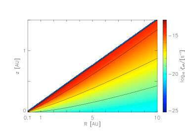
Figure 1: The effective X–ray ionisation rate $\zeta_{\rm eff}$ per hydrogen nucleus. The contour lines refer to values of $\zeta_{\rm eff}$: $10^{-15}$, $10^{-17}$, and $10^{-19}\ \rm s^{-1}$.

Figure 2: Vertical profiles of the magnetic Reynolds numbers $\rm Re_{m}$. The profile drawn with the solid line refers to the profile used by Fleming & Stone (2003) in their model with a small dead zone. The two dashed lines correspond to profiles used by Turner et al. (2007) in their models F1 and F56. The profile drawn with the dotted line refers to our model1, calculated at $R=10\ \rm AU$ and a metal abundance of $x_{\rm Mg}=5\times 10^{-11}$. Details are discussed in the text.

5 Previous simulations of dead zones

As has been well documented in the literature, there remain questions about the applicability of the MRI to protostellar discs because of their high densities and low temperatures, which lead to low levels of ionisation (e.g. Blaes & Balbus 1994; Gammie 1996). The first fully non linear study of the MRI including the effects of resistivity were performed by Fleming et al. (2000), who employed shearing box simulations to examine the conditions under which fully developed turbulence could be sustained. They showed that the important quantity that determines the outcome is the magnetic Reynolds number, $\rm Re_{m}$, defined by:

$${\rm Re}_{\rm m}=\frac{Hc_{s}}{\eta}$$ (13)

where the resistivity, $\eta$, is defined by Eq. (9). Simulations showed that turbulence could only be sustained if the Reynolds number was greater than a critical value, $\rm Re_{m}^{crit}$, where this critical value depends on the magnetic field topology. For zero net flux fields $\rm Re_{m}^{crit}\simeq 10^{4}$, whereas for net vertical fields $\rm Re_{m}^{crit}\simeq 100$. The implication of this study is that protostellar discs, in which the magnetic field is an internally generated zero net flux field, will sustain turbulence in their surface regions where the ionisation degree causes $\rm Re_{m}\ga 10^{4}$, but will remain in a near–laminar state in regions near the midplane, as envisaged by the layered disc model of Gammie (1996).

Shearing box simulations of stratified protostellar discs, with resistivity varying with height, were presented by Fleming & Stone (2003). Calculations were presented with different vertical resistivity and magnetic Reynolds number profiles, and it was shown that layered accretion resulted when the magnetic Reynolds number satisfied $\rm Re_{m}>Re_{m}^{crit}$ in the surface layers, with $\rm Re_{m}<Re_{m}^{crit}$ in the midplane regions. Their results also showed that a low Reynolds stress could be sustained in the dead zones due to the penetration of sound waves excited in the overlying active regions. The magnetic Reynolds number profile assumed in the simulation for a “small dead zone” from Fleming & Stone (2003) is shown by the solid line in Fig. 2. The magnetic Reynolds number varies from 1000 at the midplane, to $9.23\times 10^{5}$, $1.31\times 10^{7}$, and $1.62\times 10^{8}$ at $z/H=1$, $z/H=2$, and $z/H=3$, respectively, resulting in a simulated disc with a dead zone whose vertical height is $\ll H$.

In a recent paper, Turner et al. (2007) have presented a study of dead zones which included shearing box simulations of vertically stratified discs with resistivity varying as a function of height, and also a multifluid simulation in which the resistivity was able to change locally because of chemical evolution of the gas. In this study, Turner et al. (2007) employed the reaction network given by Eqns. (1) – (4) in order to calculate the ionisation fraction and resistivity. For those runs in which the resistivity was kept constant in time, the initial resistivity profile was obtained from the equilibrium solutions to Eqns. (1) – (4). The run in which resistivity varied in time and space employed a multifluid approach, similar to that described in Sect. 2. Ionisation was assumed to be due to cosmic rays, and the underlying disc model was the minimum mass solar nebula model of Hayashi (1981). In Fig. 2 we present two of the resistivity profiles employed by Turner et al. (2007) corresponding to their runs F1 and F56. In run F1 the resistivity was a fixed function of height and corresponded to a radial location $R=1$ AU with the gas–phase abundance of magnesium equal to the solar abundance ($3.39\times 10^{-5}$ magnesium atoms per hydrogen nucleus, corresponding to $x[\rm Mg]\sim 6.8\times 10^{-5}$ in our units). This run led to a layered accretion flow with active surface layers and midplane dead zone, as expected from the steep resistivity profile. It was shown that the boundary between dead and active zones is well described by the criterion that MHD turbulence is sustained by the MRI if the Lundquist number $\rm Lu\equiv v_{A}^{2}/(\Omega\eta)>1$, where $v_{A}$ is the Alfvén speed. Run F56 had a resistivity profile corresponding to a disc at 5 AU with gas phase magnesium abundance equal to $10^{-6}$ below solar abundance (corresponding closely to our model with $x[\rm Mg]=5\times 10^{-11}$). This model led to a fully turbulent disc, as expected from the flat resistivity profile obtained because the disc provides less shielding of cosmic rays at 5 AU.

The multifluid model presented by Turner et al. (2007), in which the chemistry was evolved simultaneously with the dynamics, led to an interesting and somewhat unexpected result. This disc model corresponded to the radial position $R=1$ AU in the disc, and assumed a gas–phase magnesium abundance equal to the solar value. During the early phase of the model, the disc showed the expected layered structure with dead zone near the midplane, and active zone near the disc surface. After about 60 orbits the situation changed after a period of more intense mixing caused by enhanced turbulent activity. The recombination time then exceeded the mixing time, allowing free electrons to mix toward the midplane, where net radial and azimuthal fields had built up due to field of the opposite polarity advecting through the vertical boundaries. The presence of these net magnetic fields leads to an enhance magnetic stress that partially enlivens the dead zone during periods when the ionisation fraction has been increased.

In this paper, we assume that the ionisation of the disc material arises because of X-rays that originate in the corona of the central T Tauri star. We neglect contributions from Galactic cosmic rays, as it remains an open question whether or not they can to penetrate into disc regions we consider. The X–ray ionisation rate decreases with cylindrical radius $R$, because the X-ray optical depth along the line of sight increases as one moves out into the disc.
Our use of strictly periodic boundary conditions in the vertical direction, along with an initial magnetic field that has zero net flux, means that the net flux remains zero throughout the simulations. The expectation then is that turbulence will be sustained only in those regions where the magnetic Reynolds number $\rm Re_{m}\ga 10^{4}$, and we do not expect that large scale net–flux magnetic fields will be able to accumulate in the dead zones of our simulations. As such we do not expect to observe the behaviour shown by simulation V1 of Turner et al. (2007). We now present the results from a series of systematic experiments which examine the effects of chemical evolution and turbulent mixing on the evolution of the MRI.

6 Simulation results

In this section we present the results of our multifluid MHD simulations which examine the role of turbulent mixing on the structure of dead zones. The primary aim of these simulations is to demonstrate that there exists a region of parameter space in which turbulent mixing can enliven a dead zone which is otherwise predicted to exist in models that neglect turbulent transport. A further aim is to demonstrate good agreement between MHD simulations and the predictions of a simple reaction–diffusion scheme. This latter issue is addressed in Sect. 6.3.

When discussing the results of our simulations we will often refer to certain averaged quantities. We use the same averaging procedures presented in recent publications studying vertically stratified disc models (e.g. Stone et al. 1996; Flemming & Stone 2003; Fromang & Papaloizou 2006). The azimuthal and radial average of quantity $f({\bf r},t)$ at a given time $t$ is defined by

$$F^{\ast}(z,t)=\left(f\right)^{\ast} = \frac{\int\!\!\!\int f(x^{\prime},y^{\prime},z,t)\ \mathrm{d}x^{\prime}\ \mathrm{d}y^{\prime}}{\int\!\!\!\int\mathrm{d}x^{\prime}\ \mathrm{d}y^{\prime}}$$

and the volume average is given by

$$F^{\ast\ast}(t)=\left(f\right)^{\ast\ast} = \frac{\int\!\!\!\int\!\!\!\int f(x^{\prime},y^{\prime},z^{\prime},t)\ \mathrm{d}x^{\prime}\ \mathrm{d}y^{\prime}\ \mathrm{d}z^{\prime}}{\int\!\!\!\int\!\!\!\int\mathrm{d}x^{\prime}\ \mathrm{d}y^{\prime}\ \mathrm{d}z^{\prime}}\hskip 28.45274pt.$$

where the symbols $\left(f\right)^{\ast}$ and $\left(f\right)^{\ast\ast}$, denote the corresponding averaging procedures. The time–averaged values are denoted by $\overline{\left(f\right)^{\ast}}$ and $\overline{\left(f\right)^{\ast\ast}}$.

A measure of the effective shear stress generated by the turbulence is given by the parameter $\alpha$, which has contributions from both the Reynolds and Maxwell stresses:

$$\alpha=\alpha_{\rm Rey}+\alpha_{\rm Max}$$ (14)

where

$$\alpha_{\rm Rey}(x,z) = \frac{T_{r\Phi}^{\rm Rey}}{P_{0}}=\frac{1}{P_{0}}\varrho\left(v_{x}-\langle v_{x}\rangle\right)\left(v_{y}-\langle v_{y}\rangle\right)$$ (15)

$$\alpha_{\rm Max}(x,z) = \frac{T_{r\Phi}^{\rm Max}}{P}=\frac{-\langle B_{x}B_{y}\rangle}{4\pi P_{0}}\ ,$$ (16)

and the azimuthal average (over $y$) is denoted by angled brackets, and $P_{0}$ is the initial midplane pressure. We regularly use the volume and time averaged values of $\alpha$ when discussing the simulation results below.

Table 2: List of models considered. Note that the column “recombination process included” specifies whether or not recombination of free electrons occurs along with dynamical evolution.

model	resistivity	recombination process included
model1	$\partial_{t}\eta(t,z)=0$	no
model2	$\partial_{t}\eta(t,z)\neq 0$	yes
model3	$\partial_{t}\eta(t,z)\neq 0$	no

In the following simulations we consider three different treatments of the resistivity and chemistry, and we refer to these models as model1, model2 and model3. We describe each of these below, and each are summarised in table LABEL:table:2.

1) model1: This model assumes a static resistivity profile which varies with height. The resistivity profile at $t=0$ is obtained using the equilibrium solution of the kinetic model presented in Eqns. (1) – (4). During the simulations the local resistivity values are kept fixed. This model corresponds to the single fluid models of Fleming & Stone (2003), and the runs F1, F52, F56, F58 of Turner et al. (2007).
2) model2: This is a multifluid model in which the resistivity varies in both time and space. The chemical reaction network given by Eqns. (1) – (4) is solved simultaneously with the dynamical evolution. The resistivity profile at $t=0$ is obtained from the equilibrium solution of the kinetic model.
3) model3: This is a multifluid model which has a resistivity profile which varies in time and space. The resistivity profile at $t=0$ is obtained using the equilibrium solution of the kinetic model presented in Eqns. (1) – (4). For $t>0$, however, the recombination of free electrons with ions is switched off, as is further ionisation of neutral species by X–rays. Local changes in the resistivity are due only to the turbulent mixing of ions. This model is equivalent to one in which the initial values of resistivity are conserved on fluid elements by being advected with the flow.

We now present our simulation results in detail. We begin by highlighting simulations which show that turbulent mixing can remove the dead zone, before examining disc evolution at different radii and with different magnesium abundances.

6.1 Dead–zone removal through turbulent mixing

Figure 3: model1/model2 - Time averaged vertical profiles of the horizontally averaged density, normalised Maxwell and Reynolds stresses $T_{R\Phi}/P_{0}$, and plasma parameter $\beta$. The profiles on the left refer to the results obtained with the model assuming a fixed resistivity (model1). Results obtained with model2 are shown in the right panels. Both shearing box models are calculated for $R=10\ \rm AU$ and $x_{\rm Mg}=5\times 10^{-11}$. $\alpha_{\rm Max}$ (solid line) and $\alpha_{\rm Rey}$ (dashed - dotted line) refer to a time average taken over [100,200] orbits (for model1) and [0,100] orbits for model2. For all the other quantities, the time averages are taken over 10 orbit intervals, starting from $t=0$ (dashed line). For model1 the solid line denotes averages takenbetween $t=[140,150]$ orbits, and for model2 the solid lines represented averages taken between $t=[90,100]$ orbits. The dotted lines refer to time averages taken over $t=[0,10],\ [10,20],\ \cdots,[80,90]\,{\rm for\ \texttt{model2}},\ \cdots,[130,140]$ for model1.

Figure 4: model1/model2 - Time averaged vertical profiles of the horizontally averaged kinetic energy, $0.5\varrho v^{2}/P_{0}$, and the magnetic energy $B^{2}/(8\pi P_{0})$. The profiles on the left panel show results obtained assuming a fixed resistivity profile (model1), while the results obtained with model2 are shown in the right panels. Both shearing box models are calculated for $R=10\ \rm AU$ and $x_{\rm Mg}=5\times 10^{-11}$. The time average is taken over 10 orbit intervals, starting from $t=0$ (dashed line) toward the interval $t=[90,100]$ (solid line, model2) and $t=[140,150]$ (solid line, model1), respectively. The dotted lines refer to time averages taken over $t=[0,10],\ [10,20],\ \cdots,[80,90]([130,140])$ orbits.

Figure 5: model3: - Time averaged vertical profiles of the horizontally averaged value of normalised Maxwell and Reynolds stresses $T_{R\Phi}/P_{0}$, the plasma parameter $\beta$, the kinetic energy $0.5\varrho v^{2}/P_{0}$, and the magnetic energy $B^{2}/(8\pi P_{0})$. As in the previous figures, the shearing box model is calculated for $R=10\ \rm AU$ and $x_{\rm Mg}=5\times 10^{-11}$. $\alpha_{\rm Max}$ (solid line) and $\alpha_{\rm Rey}$ (dashed - dotted line) refer to a time average taken over [0,100] orbits. For all the other quantities, the time average is taken over 10 orbit intervals, starting from $t=0$ (dashed line) towards $[90,100]$ (solid line). The dotted lines refer to time averages taken over the intervals $t=[0,10],\ [10,20],\ \cdots,[80,90]$ orbits.

In this subsection we present a suite of models which demonstrate that turbulent mixing and continuing chemical evolution of the gas are able to enliven a dead zone. All three models presented in this subsection correspond to a radial location in the disc $R=10$ AU, and have a gas–phase magnesium abundance $x_{\rm Mg}=5\times 10^{-11}$. Because of the identical initial conditions used for these three models, we can identify the specific effects of the chemistry on the evolution of the MRI .
model1
The resistivity in this model is calculated from the equilibrium electron abundance predicted by the chemical model presented in Sect. 2, and is held constant throughout the simulation. The variation of magnetic Reynolds number with height is shown in Fig. 2, which shows that the resistivity profile is intermediate between that applied by Fleming & Stone (2003) in their “small dead zone” model, and the model F56 presented by Turner et al. (2007). Specifically $\rm Re_{m}$ takes the following values: $1.4\times 10^{3}$ at the disc midplane; $6.0\times 10^{3}$ at $z/H=1$; $1.4\times 10^{4}$ at $z/H=2$; $1.3\times 10^{5}$ at $z/H=3$.

In agreeement with our expectations, this simulation resulted in a disc with well-defined dead and active zones, with the boundary between these occuring at $z/H\approx 1$ where $\rm Re_{m}\simeq 6\times 10^{3}$ and $\rm Lu\simeq 1$. This dead zone is larger than that obtained by Fleming & Stone (2003) in their model whose resistivity profile is shown in Fig. 2, for which the dead zone was confined to $z/H\leq 0.4$.

The time and volume averaged sum of the Maxwell and Reynolds stresses was found to be $\overline{\alpha^{\ast\ast}}=4.89\times 10^{-3}$ when the time average was taken over the interval [20,100] orbits. When taken over an interval [100,200] orbits, the stresses were found to decrease to $\overline{\alpha^{\ast\ast}}=8.49\times 10^{-4}$. This occurs because the stresses are higher during the development of the non linear stage of evolution early on in the simulation. We note that a fully active disc is expected to have a value $\overline{\alpha^{\ast\ast}}\ga 10^{-2}$ (see later).

The vertical profiles for the horizontally averaged density $\varrho$, the $\alpha$ values associated with the Maxwell and Reynolds stresses, the plasma parameter $\beta$, the kinetic and magnetic energy are shown in the left hand panels of Figs. 3 and 4. The time averages are taken over 10 orbit intervals, starting from $t=0$ (dashed line) towards $[140,150]$ (solid line). The dotted lines refer to profiles averaged over $t=[0,10],[10,20],\ \cdots[130,140]$. For each of the profiles, the same qualitative behaviour reported in Fleming & Stone (2003) is observed:
(i) The vertical density profile remains unchanged throughout the nonlinear evolution of the MRI.
(ii) A significant decline in the magnetic field energy towards the disc midplane is observed as compared to surface regions; $\beta$ at $z/H=0$ is between 2 and 3 orders of magnitude greater than in the active zones.
(iii) Dominance of the Reynolds stress over the Maxwell stress is observed in dead zones, due to the penetration of sound waves emitted in the overlying active zones, while the Maxwell stress is the dominant mechanism by which transport in active zones occurs. The transition occurs at $z/H\simeq 1$ where the cross-over between active and dead zones occurs.
model2
In this model the initial free electron abundance and resistivity profile is calculated from the equilibrium solution to Eqns. (1) – (4). The full set of multifluid equations, and the chemical network, are evolved together so that the local resistivity can change through turbulent transport of ions and chemical evolution (recombination/ionisation) of the gas. For this model we estimate that the turbulent mixing time corresponding to $\alpha\simeq 0.01$ is shorter than the recombination time, such that chemical mixing should enliven the dead zone. This is indeed what we find, as the simulation results in a turbulent flow which fills the entire volume of the disc, with $\overline{\alpha^{\ast\ast}}=1.31\times 10^{-2}$, where the time average was performed in the interval [20,100] orbits. We plot the vertical profiles of the various physical quantities that we have already described for model1 in Figs. 3 and 4. Comparing the figures for model1 and model2 we can make the following observations:
(i) The mean vertical density profile remains approximately constant in both models.
(ii) Whereas the Reynolds stress dominates near the midplane in model1 and the Maxwell stress dominates in the disc surface layers, we see that the Maxwell stress is dominant throughout in model2.
(iii) The plasma $\beta$ parameter is found to become very high ($\beta\simeq 10^{5}$) in the midplane of the disc in model1 as the magnetic field strength there becomes very low, whereas it remains in the range $10\leq\beta\leq 10^{3}$ for $|z/H|\leq 2$ for model2, indicative of a fully active disc.
(iv) The kinetic energy throughout the disc, but especially near the midplane, is much higher in model2 than in model1 as the turbulent velocity field is driven by the MRI.
(v) The magnetic energy near the disc midplane for model2 is more than two orders of magnitude greater than for model1 due to the continuing dynamo action associated with the MRI.
We conclude that model2 shows unambiguously that the dead zone in the disc can be removed by turbulent mixing and continuing chemical evolution under circumstances where the local mixing time scale is smaller than the recombination time, in basic agreement with the prediction of the reaction–diffusion model presented in paper II.

model3
At $t=0$ the initial resistivity profile is set up in the same way as described for model1 and model2. For $t>0$, the local resistivity is updated after every MHD time step because of the transport of free electrons and ions only. Due to the inhibition of recombination and ionisation in this model, free electrons diffuse and cause the resistivity to become homogeneous on long time scales. In the presence of sufficient numbers of free electrons in the initial ionisation state of the disc, we expect that mixing will lead to a fully active disc, and indeed this is what we find. Instead of the two–layer structure obtained using model1 above, with dead and active zones, the MHD turbulence now fills the full vertical extent of the disc. For $t>40$ orbits, we observe a quasi steady state characterised by small fluctuations around the mean value $\overline{\alpha^{\ast\ast}}=5.75\times 10^{-3}$, where the time average was taken in the interval [20,100] orbits. The vertical profiles of various quantities are shown in Fig. 5. Compared with the results obtained for model1, we see that the volume averaged turbulent stresses in each case are very similar, even though model1 had a dead zone. The reason for this is that the resistivity in model3 is higher near the disc surface because of mixing, and so reduces the strength of the turbulence there. The subsequent enlivening of the midplane in model3 does not lead to a substantial increase in the overall stress because the now–uniform resistivity is sufficient to damp the strength of the turbulence compared to its state in an ideal MHD calculation.

Comparing model3 with model2 we see that higher stresses and more vigorous turbulence are generated by model2. This is because model3 generates a disc without a dead zone, but in which the resisivity is higher than for model2, such that the strength of the resulting turbulence is suppressed somewhat. The results for model3 show that mixing the initial free electron population throughout the disc can cause the dead zone to disappear, but that allowing the chemical evolution of the disc to continue during the turbulent mixing leads to a more active disc. This is because the continuing ionisation of species near the disc surface, followed by mixing toward the midplane, produces a higher ionisation fraction overall.

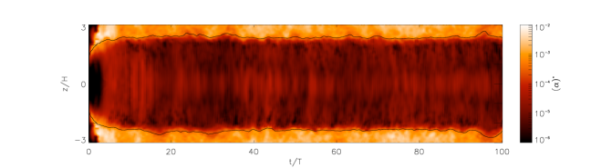
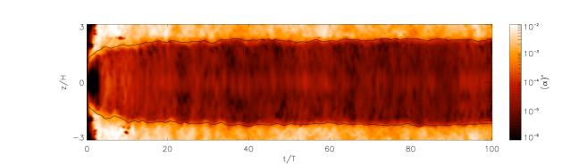
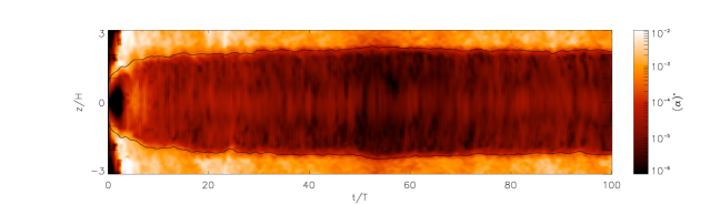
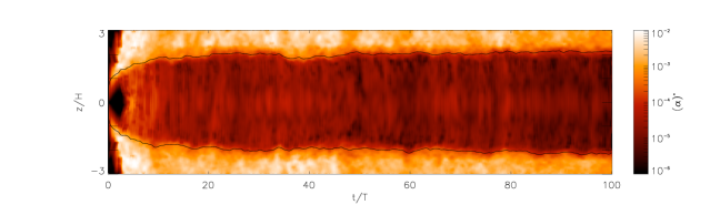
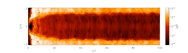
Figure 6: model2: - Space-time plots of the horizontally averaged value of $\alpha$ calculated at different radial positions $R$ and a metal elemental abundance of $x_{\rm Mg}=0$. The cylindrical radius $R$ varies from 1 AU (top panel) to 10 AU (bottom panel) passing through $R\rm=3$, 5, and  7  AU. The solid line drawn at the boundary between the live and dead zones indicates the position where the horizontally averaged Lundquist number $\rm Lu=1$.

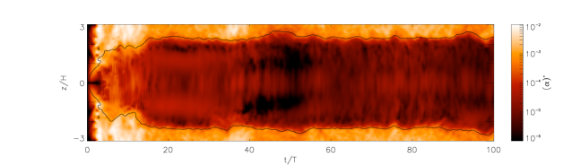
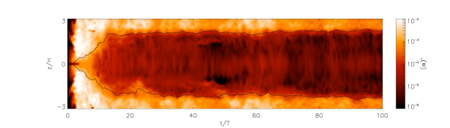
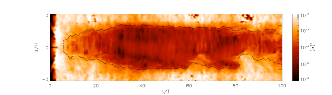
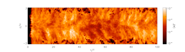
Figure 7: model2: - Space-time plots of the horizontally averaged value of $\alpha$ calculated at different radial positions $R$ and a metal elemental abundance of $x_{\rm Mg}=5\times 10^{-11}$. The cylindrical radius $R$ varies from 1 AU (top panel) to 10 AU (bottom panel) passing through $R\rm=3$, 5, and  7  AU. The solid line drawn at the boundary between the live and dead zones indicates the position where the horizontally averaged Lundquist number $\rm Lu=1$.

6.2 Results as function of $x_{\rm Mg}$ and orbital radius

A primary motivation for this paper was the indication in paper II that dead zones could be enlivened by a combination of turbulent mixing and sufficient abundance of gas–phase magnesium atoms. In that paper we presented calculations of the ionisation fraction in standard $\alpha$-discs using reaction–diffusion models. The main results were that turbulent mixing could only change the structure of a dead zone if: (i) the abundance of magnesium was sufficient (so as to increase the recombination time); (ii) one was considering locations further out in the disc where the lower temperatures and densities increase the recombination time relative to the local turbulent transport time.

The purpose of the simulations presented in the following subsections are to examine how turbulent mixing affects dead zone structure as a function of magnesium abundance and radial position in the disc, as a test of the predictions contained in paper II. We also perform a detailed comparison between some of our MHD simulations and the predictions of the reaction–diffusion model. These simulations solve the full set of multifluid equations in combination with the chemical model described in Sect. 2. We first present shearing box simulations of discs at various locations between 1 and 10 AU with gas–phase magnesium abundance equal to zero, before considering a similar set of models with gas–phase magnesium abundance $x_{\rm Mg}=5\times 10^{-11}$, which is about $10^{-6}$ of the solar value.

6.2.1 Models with $x_{\rm Mg}=0$

We begin our discussion by first examining the dead zone structure after saturation obtained for model2 with $x_{\rm Mg}=0$. We examine the disc evolution at radii $R=$ 1, 3, 5, 7 and 10 AU. In basic agreement with the results obtained in paper II, the dead zone structures obtained when magnesium is absent are very similar for all radii considered. In Fig. 6 we present space-time plots of the horizontally averaged value of $\alpha$, and it is clear that the disc sustains a two–zone structure for all radii and all time, which consists of a large dead zone which extends from the midplane to $|z/H|\simeq 2$ where the magnetic Reynolds number $\rm Re_{m}\ga 4000$ and the Lundquist number $\rm Lu\ga 1$ (shown by the solid lines in Fig. 6). Across the region bounded by $2\leq|z/H|\leq 2.3$ we find that the horizontally averaged $\alpha$ varies by more than two orders of magnitude, and this is maintained for the duration of the simulation (100 orbits).

6.2.2 Models with $x_{\rm Mg}=5\times 10^{-11}$

We now consider the dead zone structures obtained for a magnesium abundance of $x_{\rm Mg}=5\times 10^{-11}$ at radii $R=$ 1, 3, 5, 7, and 10 AU. Space-time plots of the hoizontally averaged value of $\alpha$ are shown in Fig. 7. At $R=1\ \rm AU$ and $3\ \rm AU$, the location of the boundary separating the dead from the active layer matches very well the structure obtained for $x_{\rm Mg}=0$, since the height at which $\rm Re_{m}$ begins to exceed 4000 is $|z/H|\simeq 2$ (which is also the height at which the Lundquist number $\rm Lu>1$, shown by the solid lines in Fig. 7). Significant changes in the dead zone structure start to become evident at $R\geq 5\ \rm AU$. At this radius the recombination time is similar to the turbulent mixing time, allowing the resistivity to be reduced there through the transport of free electrons into the dead zone. Over longer time scales we see that the dead zone that is established early on in the simulation starts to diminish, and between 80–100 orbits there is evidence that the dead zone size has decreased significantly. Nonetheless, at 100 orbits we find that there remains a region in the vicinity of the midplane that retains an average values of $\alpha\simeq 10^{-4}$.

By contrast, the space-time plots of the horizontally averaged value of $\alpha$ at $R=7$ and $10\ \rm AU$ show that the two–layer structure has completely disappeared, because mixing reduces the resistivity, and hence increases the magnetic Reynolds number to values $\ga 4000$. Turbulence now fills the entire computational domain which is confirmed by the time and volume averaged values of $\overline{\alpha^{\ast\ast}}$: $1.07\times 10^{-2}$ for $R=7\ \rm AU$ and $1.31\times 10^{-2}$ for $R=10\ \rm AU$.

Our results indicate that dead zones can be reduced or removed altogether through turbulent mixing. The criteria for sustaining MHD turbulence have already been discussed in the context of reaction–diffusion models in paper II, and also apply to the shearing box models considered here. These criteria are:
(i) There are sufficient metal atoms available in the gas phase so that recombination between metal ions and electrons becomes the dominant process by which the local ionisation fraction is determined.
(ii) The turbulent mixing time scale is shorter than the dominant recombination time on which free electrons are removed.

We now compare in detail the results of some of our MHD simulations with those obtained using the reaction–diffusion model presented in paper II and discussed in Sect. 3.

6.3 Comparing shearing box simulations and reaction–diffusion models

Encouraged by the good qualitative agreement obtained between the MHD simulations and the results presented in paper II, we now examine in detail the level of agreement between the simulations and the reaction–diffusion model. As mentioned in Sect. 3, we assume that the diffusion coefficient, $\cal D$, which governs the rate at which chemical species mix vertically in the disc, is equal to an effective kinematic viscosity generated by the turbulence $\nu_{m}=\alpha_{m}c_{s}^{2}/\Omega$, where $\alpha_{m}$ refers to a dimensionless parameter that measures the rate of vertical mixing (not to be confused with the value of $\alpha$ associated with the radial transport of angular momentum). When solving the reaction–diffusion equations we use a range of $\alpha_{m}$ values to obtain different solutions, which we then compare with the results of the MHD simulations. Previous work on the vertical mixing of dust grains and molecules (Carballido et al. 2005; Johansen & Klahr 2005; Turner et al. 2006; Fromang & Papaloizou 2006) suggests that the ratio of the rate of angular momentum transport to the rate of transport of chemical species by the turbulence should lie in the range $\nu/\nu_{m}\simeq 1$–3, and we examine how well our best–fit value of $\nu_{m}$ agrees with this expectation. Furthermore, the results of Turner et al. (2006) and Fromang & Papaloizou (2006) show that the diffusion coefficient is not constant with height above the midplane, but increases with height because the turbulent velocities increase in proportion to the Alfvén speed. Although we consider only a constant value of ${\cal D}$ for each reaction–diffusion model that we run, we examine the quality of the best–fit that we obtain, and quantify this by stating the error obtained in predicting the magnetic Reynolds number (which is a proxy for the free–electron abundance) at the disc midplane and surface. In general we find that using a uniform diffusion coefficient leads to a slight overestimate of the mixing rate near the midplane, and a slight underestimate near the surface.

Overall we find good agreement between the reaction–diffusion model and the MHD simulation when the value of $\alpha_{m}$ adopted in the former is between a factor of 1–2 times lowerer than the time and volume averaged value of $\alpha$ obtained in the latter. The $\alpha$ values corresponding to each MHD simulation are listed in table LABEL:table:3. The best–fit values of $\alpha_{m}$ are listed in table LABEL:table:4, along with the Schmidt number which measures $\alpha/\alpha_{m}$.

Figure 8: model2: - Comparison between vertical profiles of the magnetic Reynolds number obtained for $R\rm=5\ AU$ and $x_{\rm Mg}=0$ and $x_{\rm Mg}=5\times 10^{-11}$, respectively. Left panels show shearing box simulation results, and right panels reaction–diffusion model results. In the left panels, the time averaged vertical profiles of the magnetic Reynolds number $\overline{\rm Re^{\ast}}$ are shown by taking the time average over 10 orbit intervals, starting from $t=0$ (dashed line) towards $[90,100]$ (solid line). The other profiles (dotted lines) refer to the intervals $t=[0,10],\ [10,20],\ \cdots[80,90]$ orbits. The resistivity profiles of the magnetic Reynolds number $\rm Re_{m}$ shown in the right panels refer to the equilibrium profiles obtained with the reaction–diffusion model assuming different values of $\alpha_{m}$. In particular for $x_{\rm Mg}=0$, the value of the magnetic Reynolds number is not affected by the actual value of $\alpha_{m}$, leading to identical profiles for $\alpha_{m}=0$, $\alpha_{m}=10^{-3}$, and $\alpha_{m}=10^{-2}$. Note that both shearing box simulations and the reaction–diffusion models are initiated with the steady state profile obtained for $\alpha_{m}=0$.

We have compared the results of models located at disc radii $R=5$, 7 and 10 AU, and with magnesium abundances $x_{\rm Mg}=0$ and $x_{\rm Mg}=5\times 10^{-11}$. In each case we examine how the vertical profile of the magnetic Reynolds number $\rm Re_{m}$ evolves with time, and in the case of the reaction–diffusion model we calculate the equilibrium value of $\rm Re_{m}$ from the underlying ionisation fraction. In each case we initiate the calculation assuming that the initial chemical abundance profile is equal to the equilibrium state in the absence of mixing. For each disc radius, we plot the profile of the evolving $\rm Re_{m}$ below. In the left panels we present the results from the MHD simulations, and in the right panels the equilibrium profile from the corresponding reaction–diffusion model assuming different values of $\alpha_{m}$. The values of $\rm Re_{m}$ plotted for shearing box simulations are horizontal and time averages, where each time average was performed over 10 orbit intervals. We plot the initial value of $\rm Re_{m}$ using the dashed line, and subsequent values are plotted using dotted lines starting at $t=[0,10]$ and moving up to $t=[80,90]$. The final values at $t=[90,100]$ are shown using the solid line.

Figure 9: model2: - Comparison between vertical profiles of the magnetic Reynolds number obtained for $R\rm=7\ AU$ and $x_{\rm Mg}=0$ and $x_{\rm Mg}=5\times 10^{-11}$, respectively. Left panels show shearing box simulation results, and right panels reaction–diffusion model results. In the left panels, the time averaged vertical profiles of the magnetic Reynolds number $\overline{\rm Re^{\ast}}$ are shown by taking the time average over 10 orbit intervals, starting from $t=0$ (dashed line) towards $[90,100]$ (solid line). The other profiles (dotted lines) refer to the intervals $t=[0,10],\ [10,20],\ \cdots[80,90]$ orbits. The resistivity profiles of the magnetic Reynolds number $\rm Re_{m}$ shown in the right panels refer to the equilibrium profiles obtained with the reaction–diffusion model assuming different values of $\alpha_{m}$. In particular for $x_{\rm Mg}=0$, the value of the magnetic Reynolds number is not affected by the actual value of $\alpha_{m}$, leading to identical profiles for $\alpha_{m}=0$, $\alpha_{m}=10^{-3}$, and $\alpha_{m}=10^{-2}$. Note that both shearing box simulations and the reaction–diffusion models are initiated with the steady state profile obtained for $\alpha_{m}=0$.

Table 3: Time and volume averaged values of $\overline{\alpha^{\ast\ast}}$ obtained for the models described in the paper. The first column gives the model label and the cylindrical radius considered. The values of $\overline{\alpha^{\ast\ast}}$ are listed in the $2^{\rm nd}$ and $3^{\rm rd}$ column assuming a elemental metal abundance $x_{\rm Mg}$ of 0 and $5\times 10^{-11}$, respectively. Apart from the value denoted with the symbol †, the time average was taken over [20,100] orbits, while ()^† refers to the time average taken over [100,200] orbits.

	$\overline{\alpha^{\ast\ast}}(x_{\rm Mg}=0)$	$\overline{\alpha^{\ast\ast}}(x_{\rm Mg}=5\cdot 10^{-11})$
model1
at $10\ \rm AU$		$4.89\cdot 10^{-3}$
		$(8.49\cdot 10^{-4})^{{\dagger}}$
model3
at $10\ \rm AU$		$5.75\cdot 10^{-3}$
model2
at  $1\ \rm AU$	$2.67\cdot 10^{-4}$	$2.51\cdot 10^{-4}$
at  $3\ \rm AU$	$3.01\cdot 10^{-4}$	$3.46\cdot 10^{-4}$
at  $5\ \rm AU$	$2.84\cdot 10^{-4}$	$1.11\cdot 10^{-3}$
at  $7\ \rm AU$	$5.44\cdot 10^{-4}$	$1.07\cdot 10^{-2}$
at $10\ \rm AU$	$5.10\cdot 10^{-4}$	$1.31\cdot 10^{-2}$

Table 4: Values of the diffusion coefficients applied to the reaction-diffusion model which best matches the corresponding MHD results for model2 with $x_{\rm Mg}=5\cdot 10^{-11}$. The Schmidt number $S_{c}$ is listed in the 3rd column refering to time and volume averaged values of $\overline{\alpha^{\ast\ast}}$ between [20,100] orbits.

R [AU]	$\alpha_{m}$	$S_{C}$
5	$5.89\cdot 10^{-4}$	1.88
7	$8.67\cdot 10^{-3}$	1.23
10	$9.28\cdot 10^{-3}$	1.41

Figure 10: model2: - Comparison between vertical profiles of the magnetic Reynolds number obtained for $R\rm=10\ AU$ and $x_{\rm Mg}=0$ and $x_{\rm Mg}=5\times 10^{-11}$, respectively. Left panels show shearing box simulation results, and right panels reaction–diffusion model results. In the left panels, the time averaged vertical profiles of the magnetic Reynolds number $\overline{\rm Re^{\ast}}$ are shown by taking the time average over 10 orbit intervals, starting from $t=0$ (dashed line) towards $[90,100]$ (solid line). The other profiles (dotted lines) refer to the intervals $t=[0,10],\ [10,20],\ \cdots[80,90]$ orbits. The resistivity profiles of the magnetic Reynolds number $\rm Re_{m}$ shown in the right panels refer to the equilibrium profiles obtained with the reaction–diffusion model assuming different values of $\alpha_{m}$. In particular for $x_{\rm Mg}=0$, the value of the magnetic Reynolds number is not affected by the actual value of $\alpha_{m}$, leading to identical profiles for $\alpha_{m}=0$, $\alpha_{m}=10^{-3}$, and $\alpha_{m}=10^{-2}$. Note that both shearing box simulations and the reaction–diffusion models are initiated with the steady state profile obtained for $\alpha_{m}=0$.

6.3.1 Results at 5 AU

We first discuss the results for $R=5\ \rm AU$ which are shown in Fig. 8. Note that in the upper left panel of Fig. 8, the magnetic Reynolds number shows a well defined minimum, and this arises because this MHD simulation was performed with a ceiling being adopted for the resistivity in the induction equation, corresponding to a minimum value of $\rm Re_{m}=20$. This was done to ensure that the time step constraint arising from the diffusive term in the induction equation was not too severe. The minimum value of $\rm Re_{m}$ that we calculated from the electron fraction during this simulation was $\rm Re_{m}=10.007$.

The upper left panel of Fig. 8 simply shows that the model at 5 AU with $x_{\rm Mg}=0$ maintains a significant dead zone with $|z/H|\leq 2$ (where $\rm Re_{m}\simeq 4000$) throughout, and the magnetic Reynolds number does not change from its initial value. The upper right hand panel shows that the reaction–diffusion equation agrees with this, as the single line plotted is actually three lines overplotted corresponding to $\alpha_{m}=0$, $10^{-3}$ and $10^{-2}$. In the absence of magnesium, the recombination rate is simply too high to allow mixing to modify the dead zone for $\alpha_{m}$ values in this range.

The lower left panel shows the evolution of $\rm Re_{m}$ with $x_{\rm Mg}=5\times 10^{-11}$. It is clear that the $\rm Re_{m}$ profile in this case is non stationary near the midplane, even after 100 orbits, and this appears to be because this particular model is one which maintains a dead zone throughout the run, but whose parameters are close to those which would allow mixing to remove the dead zone. Episodic increases and decreases in turbulent activity modify the ionisation state near the midplane, causing the $\rm Re_{m}$ values to oscillate about a value close to 1000.

The lower right panel shows the results from the reaction–diffusion model agree quite well with the mean $\rm Re_{m}$ profile from the MHD run, in particular when $\alpha_{m}=10^{-3}$. Inspection of table LABEL:table:3 shows that mean value of $\alpha$ obtained from the MHD run was $1.52\times 10^{-3}$. Table LABEL:table:4 shows that the best fit reaction–diffusion model has a value of $\alpha_{m}=5.89\times 10^{-4}$ (such that the Schmidt number equals 1.88). The error in the predicted value of $\rm Re_{m}$ at the midplane was 3 %, while the error at the disc surface was $\simeq 15\%$, showing good overall agreement even when a uniform diffusion coefficient is adopted in the reaction–diffusion models.

6.3.2 Results at 7 AU

The vertical profiles of $\rm Re_{m}$ obtained at $R=7$ AU are shown in Fig. 9. The upper left and right panels show results from the MHD simulation and reaction–diffusion calculation, respectively for magnesium abundance $x_{\rm Mg}=0$. Once again we see that mixing has no effect on the magnetic Reynolds number profile in the absence of magnesium, and a substantial dead zone is maintained throughout both calculations, which show excellent agreement.

The lower left and right panels show models for which $x_{\rm Mg}=5\times 10^{-11}$. Here we see that there is very significant change in the magnetic Reynolds number profile as turbulent mixing ensues. In the MHD simulation we see that the minimum value of $\rm Re_{m}$ changes from 1000 to $\simeq 4000$, which is high enough for the disc midplane to become active. The lower right panel shows good agreement with the MHD simulation when $\alpha=10^{-2}$. We see from table LABEL:table:3 that the average value of $\alpha$ from the MHD run is $1.07\times 10^{-2}$. Table LABEL:table:4 shows that the best fit reaction–diffusion model has a value of $\alpha_{m}=8.67\times 10^{-3}$ (such that the Schmidt number equals 1.23). The error in the predicted value of $\rm Re_{m}$ at the midplane was 2 %, while the error at the disc surface was $\simeq 15\%$.

Figure 11: model3: - Comparison between vertical profiles of the magnetic Reynolds number obtained for $R\rm=10\ AU$ and $x_{\rm Mg}=5\times 10^{-11}$ obtained by the shearing box simulation (left panel) and the reaction–diffusion model (right panel). The results refer to the simulation where recombination and ionisation are switched off (model3). In the left panel, the time averaged vertical profiles of the magnetic Reynolds number $\overline{\rm Re_{m}^{\ast}}$ are shown by taking time averages over 10 orbit intervals, starting from $t=0$ (dashed line) towards $[90,100]$ (solid line). The other profiles (dotted lines) refer to $t=[0,10],\ [10,20],\ \cdots[80,90]$. The resistivity profiles of the magnetic Reynolds number $\rm Re_{m}$ shown in the right panel refer to the equilibrium profiles obtained with the reaction–diffusion model assuming different values of $\alpha_{m}$. In fact, the equilibrium profile obtained for model3 is not affected by the actual value of $\alpha_{m}>0$. Note that both shearing box simulation and the reaction–diffusion model are initiated with the equilibrium profile obtained for $\alpha_{m}=0$.

6.3.3 Results at 10 AU

The profiles obtained at $R=10\ \rm AU$ are shown in Fig. 10. The upper panels are again in good agreement when $x_{\rm Mg}=0$, showing that mixing has no effect on the dead zone structure. The lower panels show that the $\rm Re_{m}$ profile is changed significantly by mixing when $x_{\rm Mg}=5\times 10^{-11}$, such that the dead zone is enlivened completely. In the MHD simulation the minimum value of $\rm Re_{m}$ changes from $\simeq 1000$ to $\simeq 6000$, allowing the dead zone to become MRI–active and the disc to be turbulent throughout its height. Good agreement in the $\rm Re_{m}$ profile is obtained using the reaction–diffusion model when $\alpha_{m}\simeq 10^{-2}$, which as expected is slightly lower than the value $\alpha=1.31\times 10^{-2}$ listed in table LABEL:table:3 as arising from the MHD simulation. Table LABEL:table:4 shows that the actual best fit reaction–diffusion model has a value of $\alpha_{m}=9.28\times 10^{-3}$ (such that the Schmidt number equals 1.41). The error in the predicted value of $\rm Re_{m}$ at the midplane was $<1$ %, while the error at the disc surface was $\simeq 15\%$, which again illustrates the fact that reasonable agreement can be obtained when using a uniform diffusion coefficient.

6.3.4 Reaction-diffusion results for model3

We finally present a comparison between the MHD simulation for model3 and a corresponding reaction–diffusion model. To recap: model3 allows the free electrons and ions to diffuse, but does not include recombination or on–going ionisation. The MHD simulation and reaction-diffusion model were initiated with the equilibrium chemical abundance for the case $x_{\rm Mg}=5\times 10^{-11}$ at $R=10$ AU. The expectation is that turbulent mixing will cause the $\rm Re_{m}$ profiles to change from their initial values to become uniform. Inspection of Fig. 11 confirms that our models agree with this expectation.

7 Conclusions

We have presented the results from a series of shearing box multifluid MHD simulations aimed at examining the evolution and structure of dead zones in protoplanetary discs, in the presence of turbulent transport of ions, on–going chemical evolution of the gas, and ionisation due to X–rays emitted by the central star. We have adopted a number of simplifying assumptions, including the absence of small grains whose presence in even modest numbers would lead to rapid removal of free electrons (Sano et al. 2000; Ilgner & Nelson 2006a). As such, our results are likely to be most applicable to protostellar discs at a fairly late stage of evolution after grains have accumulated to form larger bodies.

A primary objective of this work was to use MHD simulations to re–examine the results of Ilgner & Nelson (2006b), who used a simple reaction–diffusion model to calculate the effects of turbulent mixing on dead zone structure. The simple model predicted that turbulent transport can be effective at enlivening a dead zone provided that: (i) the abundance of gas–phase magnesium is sufficient; (ii) one considers regions of the disc beyond radii $\ga 5$ AU where turbulent mixing occurs on a shorter time scale than recombination. The main conclusions of this paper are that full multifluid MHD simulations are in good agreement with these predictions. Models simulated at radii between 1 – 10 AU, and with no magnesium in the gas–phase, showed a two–layer structure consisting of an actively accreting zone near the disc surface, and a magnetically inactive region near the midplane. The addition of gas–phase magnesium with fractional abundance $x_{\rm Mg}=5\times 10^{-11}$ led to significant dead zones persisting for radii $R\leq 5$ AU, but models at 7 and 10 AU resulted in fully active discs without dead zones. The implications for protoplanetary discs is that at late times, when most of the small submicron sized dust grains have grown to much larger sizes, the dead zone beyond 5 AU may be enlivened because of turbulent transport of ions toward the midplane. Regions interior to 5 AU will, however, retain their dead zones.

A further conclusion of our work is that detailed comparison between the simple reaction–diffusion model and the MHD simulations leads to very good agreement in the vertical profiles of resistivity and magnetic Reynolds number when an appropriate diffusion coefficient is chosen. Typically we find that the best–fit vertical diffusion coefficient corresponds to a ratio in the range 1–2 between the rate at which angular momentum is transported radially and the rate at which diffusion of chemical species occurs vertically. This result is consistent with those presented by Carballido et al. (2005), Johansen & Klahr (2005), Turner et al. (2006) and Fromang & Papaloizou (2006) who showed that turbulent diffusion of dust (and chemical tracers) occurs on a slightly slower time scale than the transport of angular momentum, since it is driven through correlations in the perturbed flow velocities only.

It has traditionally been assumed that MRI-driven MHD turbulence in discs can be sustained against the damping effects provided by ohmic resistivity if magnetic field diffusion over the characteristic wavelength of the instability occurs on a time scale longer than the growth time. Indeed Turner et al. (2007) showed that such a condition provides a good indicator of where the transition between active and dead zones in a disc will occur. They showed that the transition zone occurs where the Lunquist number ${\rm Lu}\equiv v_{A}^{2}/(\eta\Omega)\simeq 1$, and our simulation results are in good agreement with this. Recent work by Fromang & Papaloizou (2007) and Fromang et al. (2007), however, has shown that in the case of non stratified shearing box simulations, turbulence is only sustained in discs where the magnetic Prandtl number $P_{m}\equiv\nu/\eta>1$ (where $\nu$ is the physical (molecular) viscosity), even when ${\rm Lu}>1$ in the initial state. The interpretation is that MRI-driven turbulence cascades the magnetic field down to the smallest scales available, by virtue of the turbulent velocity field twisting the field up. If the characteristic scale on which velocity fluctuations are damped is smaller than the resistive scale, then a zero net flux field will be dissipated and turbulence will die. Interestingly, the magnetic Prandtl number in protostellar discs is expected to be $P_{m}<1$, since resistivity is high and viscosity is low. Fromang & Papaloizou (2007) also show that the intrinsic numerical magnetic Prandtl number of the ZEUS code is $>1$, at least for simulations with resolutions feasible on current computers. This suggests that the results in this paper, and those in other papers that have looked at dead zones, are modelling discs which only fullfil one of the necessary criteria for MHD turbulence to be sustained in a physical way, namely that ${\rm Lu}>1$. The condition for $P_{m}>1$ is satisfied because of the nature of numerical dissipation in the code. We note that the effects observed by Fromang & Papaloizou (2007) and Fromang et al. (2007) occur for the particular case of non stratified shearing box simulations, and that a mechanism for maintaining active MRI turbulence may be the generation of large scale magnetic field through magnetic buoyancy effects and field stretching in vertically stratified discs, such as those we consider in this paper. Nonetheless, it is clearly necessary to examine these issues by including the appropriate viscous as well as resistive transport coefficients in simulations, and we will do this in a future publication.

There are two additional issues that we have not addressed in this paper. The first is that scattering of X–rays toward the disc midplane may increase the ionisation rate in the disc by up to an order of magnitude (Igea & Glassgold 1999), and this can have an obvious effect on the structure of the dead zone. Although we have not undertaken an extensive analysis of the effect of this, we have run a model at 1 AU with $x_{\rm Mg}=5\times 10^{-11}$ with the X–ray luminosity increased by two orders of magnitude. We find only a small change in the dead zone structure in this case. We would expect in general that increases in the X–ray luminosity due to scattering will move the radial boundary of the dead zone inward slightly, but will not completely remove the dead zone. A final issue that we have not addressed in this paper is that of X–ray flares. Observations of T Tauri stars by CHANDRA have shown that they emit regular outbursts of X–rays which may increase the X–ray luminosity by a few orders of magnitude, and also harden the X–ray spectrum (Favata et al 2005; Wolk et al. 2005). This issue was examined by Ilgner & Nelson (2006c), who showed that the flaring could significantly modify dead zones in protoplanetary discs. We will address this issue in a future paper using multifluid MHD simulations with chemistry, so that both the effects of X–ray flaring and chemical mixing on dead zone structure can be examined.

- (1) Balbus, S., Hawley, J., 1991, ApJ, 376, 214
- (2) Balbus, S., Papaloizou, J., 1999, ApJ, 521, 650
- (3) Balbus, S., Terquem, C., 2001, ApJ, 552, 235
- (4) Beckwith, S., Sargent, A., 1996, Nature, 383, 139
- (5) Blaes, O. Balbus, S., 1994, ApJ, 421, 163
- (6) Carballido, A., Stone, J.M., Pringle, J.P., 2005, MNRAS, 358, 1055
- (7) Favata, F., Flaccomio, E., Reale, F., Micela, G., Sciortino, Shang, H., Stassub, K., Feigelson. E. D., 2005, ApJS, 160, 469
- (8) Fleming, T., Stone, J., Hawley, J., 2000, ApJ, 530, 464
- (9) Fleming, T., Stone, J., 2003, ApJ, 585, 908
- (10) Fromang, S., Papaloizou, J., 2006, A&A, 452, 751
- (11) Fromang, S., Papaloizou, J., 2007, A&A, 476, 1113
- (12) Fromang, S., Papaloizou, J., Heinemann, T., Lesur, G., 2007, A&A, 476, 1123
- (13) Furlan, E., Hartmann, L., Calvet, N., D’Alessio, P., Fraco-Hernandez, R. et al., 2006, ApJS, 165, 568
- (14) Gammie, C., 1996, ApJ, 457, 355
- (15) Glassgold, A., Najita, J., Igea, J., 1997, ApJ, 480, 344
- (16) Goldreich, P., Lynden-Bell, D., 1965, MNRAS, 130, 125
- (17) Hawley, J., Balbus, S., 1991, ApJ, 376, 223
- (18) Hawley, J., Gammie, C., Balbus, S., 1995, ApJ, 440, 742
- (19) Hayashi, C., 1981, Prog. Theo. Phys., 70, 35
- (20) Igea, J., Glassgold, A., 1999, ApJ, 518, 848
- (21) Ilgner, M., Nelson, R., 2006a, A&A, 445, 205
- (22) Ilgner, M., Nelson, R., 2006b, A&A, 445, 223
- (23) Ilgner, M., Nelson, R., 2006c, A&A, 455, 731
- (24) Johansen, A., Klahr, H., 2005, ApJ, 634, 1353
- (25) Johansen, A., Oishi, J.S., Low, M.M., Klahr, H., Henning, T., Youdin, A., 2007, Nature, 448, 1022
- (26) Le Teuff, Y., Millar, T., Markwick, A., 2000, A&A, 146, 157
- (27) Nelson, R.P., Papaloizou, J.C.B., 2003, MNRAS, 339, 993
- (28) Nelson, R.P., Papaloizou, J.C.B., 2004, A&A, 350, 849
- (29) Nelson, R.P., 2005, A&A, 443, 1067
- (30) O’Dell, C.R., Wen, Z., Hu, X., 1993, ApJ, 410, 696
- (31) Oppenheimer, M., Dalgarno, A., 1974, ApJ, 192, 29
- (32) Pessah, M.E., Chan, C.K., Psaltis, D., 2007, ApJ, 668L, 51
- (33) Prosser, C., Stauffer, J., Hartmann, L., Soderblom, D., Jones, B., Werner, M., McCaughrean, M., 1994, ApJ, 421, 517
- (34) Sano, T., Miyama, S., Umebayashi, T., Nakano, T., 2000, ApJ, 543, 486
- (35) Semenov, D., Wiebe, D., Henning, Th., 2004, A&A, 417, 93
- (36) Shakura, N., Sunyaev, R., 1973, A&A, 24, 337
- (37) Sicilia–Aguilar, A., Hartmann, L., Briceno, C., Muzerolle, J., Calvet, N., 2004, AJ, 128, 805
- (38) Stone, J., Norman, M., 1992, ApJS, 80, 753
- (39) Stone, J., Hawley, J., Gammie, C., Balbus, S., 1996, ApJ, 463, 656
- (40) Turner, N., Sano, T., Dziourkevitch, N., 2007, ApJ, 659, 729
- (41) Wolk, S.J., Harnden, F.R., Flaccomio, E., Micela, G., Favata, F., Shang, H., Feigelson. E. D., 2005, ApJS, 160, 423