Detailed Transport Investigation of the Magnetic Anisotropy of (Ga,Mn)As

Abstract

This paper discusses transport methods for the investigation of the (Ga,Mn)As magnetic anisotropy. Typical magnetoresistance behaviour for different anisotropy types is discussed, focusing on an in depth discussion of the anisotropy fingerprint technique and extending it to layers with primarily uniaxial magnetic anisotropy.

We find that in all (Ga,Mn)As films studied, three anisotropy components are always present; The primary biaxial along ([100] and [010]) along with both uniaxial components along the [$\overline{1}$10] and [010] crystal direction which are often reported separately. Various fingerprints of typical (Ga,Mn)As transport samples at 4 K are included to illustrate the variation of the relative strength of these anisotropy terms. We further investigate the temperature dependence of the magnetic anisotropy and the domain wall nucleation energy with the help of the fingerprint method.

As the sophistication of spintronic device investigations continues to rapidly grow, a deeper and more detailed characterization of the ferromagnetic semiconductor material used in the elaboration of many of these structures is becoming ever more essential to properly understanding the operation and design of device elements. The spin-orbit mediated coupling of magnetic and semiconductor properties in these materials gives rise to many novel transport-related phenomena which can be harnessed for device applications. For the understanding and reliable functioning of such devices it is important to understand and be able to determine the magnetic anisotropy of the parent layer and of readily structured samples. While FMR [1] and SQUID [2] can effectively measure the main magnetic anisotropy of the parent layer, they are not practical for anisotropy studies on individual small structures which have too little magnetic moment to be detected. Transport measurements, on the other hand provide a very effective means of extensively studying the anisotropy at a fixed temperature. Using a vector field magnet, many magnetic field scans in different in-plane (or even space-) directions can be recorded within a short time frame without remounting the sample. Anisotropic transport properties allow for electrical monitoring of the magnetization. This provides detailed information on the angular dependence of the magnetic behaviour.

A technique for extracting the magnetic anisotropy by transport means was introduced in [3]. In this treatise we discuss investigations of the magnetization behaviour by tranport means in general and in particular the anisotropy fingerprint technique in much greater detail. We present a variety of fingerprints of different (Ga,Mn)As layers at 4 K and discuss the always present three symmetry components of the magnetic anisotropy at 4 K. We then extend the method to the case of a uniaxial material, which is necessary to describe (Ga,Mn)As layers at higher temperatures or structured submicron devices. We investigate the temperature behaviour of the (Ga,Mn)As anisotropy using the fingerprint method. It shows the typical transition from a mainly biaxial system at low temperature to a uniaxial system close to T_C. From these fingerprints we can also extract the temperature dependence of the domain wall nucleation and propagation energy.

1 Anisotropic Transport and Magnetic Anisotropy in (Ga,Mn)As

The ferromagnetic semiconductor (Ga,Mn)As is strongly anisotropic both in transport and in its magnetic properties. It shows a strong anisotropic magnetoresistance effect (AMR): The resistivity for a current flow perpendicular to the magnetization $\rho_{\bot}$ is larger than $\rho_{||}$ parallel to the magnetization[4]. Ohm’s law is best expressed with the electric field E broken up in components parallel and perpendicular to the magnetization M [5, 6]

$$\mathbf{E}=\rho_{||}\mathbf{J_{||}}+\rho_{\bot}\mathbf{J_{\bot}}$$ (1)

with J the current density. The projection onto the current path gives the longitudinal resistivity $\rho_{xx}$ (longitudinal AMR effect):

$$\rho_{xx}=\rho_{\bot}-(\rho_{\bot}-\rho_{||})\cos^{2}(\vartheta),$$ (2)

where $\vartheta$ is the angle between M and J. The dependence of the Hall resistivity $\rho_{xy}$ (transverse AMR or Planar Hall effect PHE) on the magnetization direction follows directly from the electric field component perpendicular to the current path:

$$\rho_{xy}=-\frac{\rho_{\bot}-\rho_{||}}{2}\sin(2\vartheta),$$ (3)

With the help of longitudinal AMR and PHE measurements it is thus possible to monitor the magnetization direction $\vartheta$ and conclude on the magnetic anisotropy of the material.

The cubic anisotropy of the crystal structure is reduced by growth strain. Here we discuss highly doped not annealed (Ga,Mn)As layers grown under compressive strain on GaAs (001) substrates. For standard thickness and experimentally relevant hole densities, the growth strain results in an additional strong hard axis in growth direction that confines the easy axes to the layer plane. This in-plane anisotropy is strongly temperature dependent as will be discussed in section 4. At 4 K the material shows a main biaxial magnetic anisotropy with easy axes along the [100] and [010] crystal direction. The above is well understood, however, in addition to this two uniaxial anisotropy terms have been observed the origin of which is not clear. One additional uniaxial anisotropy term with easy axis along [110] or $[\overline{1}10]$ is typically present and has been seen in many laboratories. A much smaller additional uniaxial anisotropy component with easy axis along [010] or [100] [7] has often been overlooked, because it is typically too small to be visible in standard SQUID measurements. Recently, the anisotropy fingerprint technique [3] allowed us to show that all three, the main biaxial and the two uniaxial, anisotropy components are simultaneously present in typical (Ga,Mn)As layers at 4 K. Section 2.1 explains the details of the method. Fingerprints of typical (Ga,Mn)As layers are shown in section 2.4 to discuss the typical relative strength of the anisotropy components and their variation from layer to layer.

In this context it is helpful to note that for the purpose of calculating the magnetostatic energy in the single domain model, any linear combination of uniaxial anisotropy components with different easy axes can be expressed as a linear combination of a [$\overline{1}$10] and a [010] uniaxial anisotropy term. It is known that:

$$a\sin\alpha+b\cos\alpha=\sqrt{a^{2}+b^{2}}\cdot\sin(\alpha+\beta),$$ (4)

where $\beta$ is given by $\arctan(b/a)$ and $\arctan(b/a)\pm\pi$ if $a\geq 0$ and $a<0$ respectively. This relates two sine functions of the same period but with different phase to a third sine function with the same period and a new phase. Consequently, we can express any combination of two uniaxial anisotropy components in a (Ga,Mn)As layer by an equivalent linear combination of the [$\overline{1}$10] and the [010] uniaxial anisotropy term. The choice of only these two directions is thus fully general and does not exclude other uniaxial anisotropy components, e.g. due to specific strain conditions in a specific sample.

Summing up the three anisotropy terms of different symmetry, we can express the magnetostatic energy E of a magnetic domain with magnetization orientation $\vartheta$ with respect to the [100]-crystal direction:

$$E=\frac{K_{cryst}}{4}\sin^{2}(2\vartheta)+K_{uni[\overline{1}10]}\sin^{2}(\vartheta-135^{\circ})+K_{uni[010]}\sin^{2}(\vartheta-90^{\circ})-MH\cos(\vartheta-\varphi),$$ (5)

where the last term is the Zeeman energy. The anisotropy constants $K_{cryst}$ in the biaxial anisotropy term and $K_{uni[\overline{1}10]}$ and $K_{uni[010]}$ in the two uniaxial terms depend differently on the magnetization M and thus on temperature[2]. This results in a characteristic temperature dependence of the overall magnetic anisotropy of the layer. This typical transition from mainly biaxial behaviour at 4 K to uniaxial behaviour close to the Curie temperature is investigated with the anisotropy fingerprint technique in section 2.1.

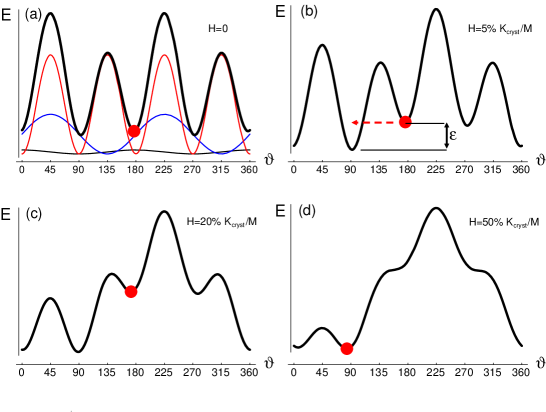
Figure 1: Energy landscape at zero field (a). The symmetry components of the anisotropy are shown with thin lines (biaxial red; uniaxial along $[\overline{1}10]$ blue; uniaxial along [010] black). The energy surface evolves with increasing field along $45^{\circ}$ (b-d) causing magnetization reversal through domain wall nucleation and propagation (b) or through Stoner-Wohlfarth rotation (c and d).

Fig. 1 shows the energy landscape, a plot of the energy of a magnetic domain as a function of the magnetization angle, and how it evolves with magnetic field. Under an applied magnetic field, the magnetization can reverse through two mechanisms. One mechanism is called coherent (Stoner-Wohlfarth [8]) rotation: With increasing magnetic field the magnetization (marked with a red dot in Fig. 1) follows the local minimum of the energy surface until the minimum disappears as illustrated in panel b to d. The dashed arrow in panel b, on the other hand, illustrates the reversal by DW nucleation and propagation. It appears if the energy gained by reorienting the magnetization direction to another local minimum of the energy surface is larger than the DW nucleation/propagation energy $\varepsilon$. A DW is nucleated and a new domain with the new magnetization orientation grows until it extends over the whole structure. As will become evident, the inherent behaviour of (Ga,Mn)As is generally dominated by Stoner-Wohlfarth rotation at high magnetic fields and by DW-nucleation/propagation related events at low fields.

2 Monitoring the Magnetization Behaviour in Transport

The described magnetization behaviour can be observed in direct or indirect magnetization measurements, and leads to a very characteristic two-step reversal process in SQUID and magnetoresistance measurements. Three-jump magnetic switching is also possible in very specific situations[9].

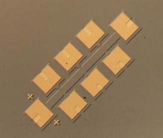
Figure 2: Hall bar structure typical of those used in this study, processed by optical lithography and dry etching. The contacts are established by gold deposition. This bar is 40 $\mu$m wide and 540 $\mu$m long.

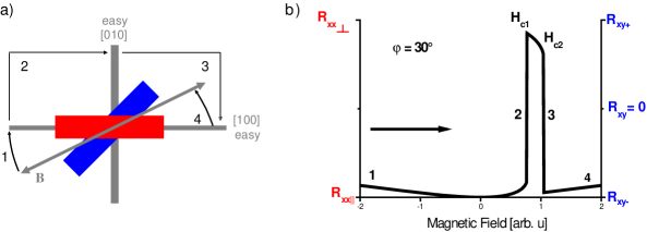
Figure 3: Two-step magnetization reversal. a) Sketch showing the magnetization behaviour in hard (blue) and easy (red) axis Hall bars. b) The corresponding calculated AMR scan for the easy axis Hall bar (left scale), which is equivalent to a Planar Hall scan on the hard axis bar (right scale).

Here we will discuss the characterization of the magnetic anisotropy of typical Ga_1-xMn_xAs transport layers. The layers were grown by low-temperature molecular beam epitaxy (LT-MBE, 270^∘C) on a high-quality GaAs buffer on an epiready semiinsulating GaAs (001) substrate. They contain between x=2% and 5% Mn and show an as-grown T_C around 50 K or above. All layers were patterned into 40 to 60 $\mu$m wide Hall bar structures as shown in Fig. 2 by optical lithography and chlorine assisted dry etching. Contacts are established through metal evaporation and lift off. During the processing care is taken to not expose the samples to any annealing treatment.

Assume a biaxial magnetic anisotropy with easy axes along the in-plane $\langle 100\rangle$ crystal directions (coordinate axes in Fig. 3a) as a first approximation of the 4 K anisotropy of (Ga,Mn)As. Assume further that the longitudinal resistance of a Hall bar with its current along the [100] axis is measured while the external magnetic field is swept from a high negative to a high positive value along a direction 30^∘ away from the [100] axis. Using eq. 5 and 2 we can now calculate the corresponding AMR signal shown in Fig. 3b(left y-axis scale). At high negative fields, the magnetization is forced along the field direction (not shown). (1) As the field is decreased M gradually relaxes through Stoner-Wohlfarth rotation until it is aligned with its closest easy axis. At zero field M is thus parallel to $[\overline{1}00]$ and to the current, yielding the smallest resistance value $R_{||}$. (2) At a small positive field H_c1 a 90^∘-DW is nucleated and propagates through the structure resulting in an abrupt change of the magnetization direction to the [010] direction. M is now perpendicular to the current, yielding the maximum resistance value R_⊥. (3) At the second switching field H_c2, another 90^∘-DW is nucleated and the magnetization jumps close to the [100] easy axis. (4) With increasing magnetic fields M rotates again towards the magnetic field direction. The entire process is of course hysteretically symmetric (not shown).

If another Hall bar is oriented along the [110] crystal direction (blue in Fig. 3a) the easy axes [100] and [010] have an angle of $\pm 45^{\circ}$ with the current path. An abrupt switch of magnetization from one easy axis to the other corresponds according to eq. 3 to a sharp switching event between two extrema of the transverse resistance. The calculated Planar Hall signal is thus up to a constant identical with the previously discussed curve in Fig. 3b, in this case centered around zero transverse resistance (blue/right y-axis). Because of this, transverse resistance measurements are the method of choice for Hall bars oriented along a crystalline hard axis. For Hall bars along an easy axis, longitudinal resistance measurements are the only useful technique. Indeed, if the current direction is rotated by 45^∘, Eq. 3 transforms into Eq. 2 (plus an uninteresting offset).

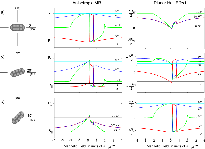
Figure 4: Calculated Anisotropic Magnetoresistance (middle) and Planar Hall effect (right) curves for magnetic field sweeps along several in-plane angles ($\varphi$= 0^∘, 30^∘, 45.1^∘, 60^∘ and 90^∘) for Hall bar orientations as indicated in the sketches on the left, with current along a) 0^∘ b) 20^∘ c) 45^∘. The underlying magnetic anisotropy is biaxial with easy axes along [100] and [010]. All angles with respect to the [100] crystal direction. The domain wall nucleation/propagation energy $\varepsilon$ is exaggerated with 30% of $K_{cryst}$.

Fig. 4 shows AMR (middle) and Planar Hall effect (right) curves for field sweeps along different angles $\varphi$ in the plane calculated using Eq. 5 in combination with Eq. 2 and 3 respectively. The domain wall nucleation energy $\varepsilon$ was exaggerated in these calculations (30% of $K_{cryst}$ instead of 5-10% as would be typical for (Ga,Mn)As)) to illustrate both Stoner-Wohlfarth rotation and DW-related magnetization switching in the same figure. The middle panel of Fig. 4a, shows MR curves for a Hall bar along a biaxial easy axis. If the external magnetic field is swept along the [100] easy axis (0^∘), the magnetization is always parallel to the current direction. The resistance (black line) thus takes its lowest value R_|| throughout the whole field range. If the field is swept along the [010] easy axis (90^∘), the magnetization is always perpendicular to the current resulting in a high resistance value R_⊥ throughout the whole curve (thin cyan). For intermediate magnetic field angles, the magnetization is parallel to the field at high positive and negative fields, yielding intermediate resistance values. At zero field the magnetization relaxes to the closest easy axis, which is [100] for the 30^∘ scan and [010] for the 60^∘ and 45.1^∘ scans, corresponding to the lowest and highest resistance value respectively. The 45.1^∘-scan (green line) can be used to measure the strength of the magnetic anisotropy. We can read out the anisotropy field (-2$K_{cryst}/M$), at the point where the magnetization starts to turn away from the magnetic field direction. A measurement with two possible resistance states at zero field always suggests a biaxial magnetic anisotropy. However, note that these two states can correspond to the same resistance value as, e.g., if the easy axis and the current include an angle of 45^∘ (left panel of Fig. 4c), where the 0^∘(black) and $90^{\circ}$(cyan) curve fall on top of each other. The panels on the right show the calculated Planar Hall resistance curves in the respective configurations. Note, that, the AMR signal in Fig. 4a is identical to the PHE signal in Fig. 4c, as discussed above. The easy axis showing constant resistance throughout the whole scan can easily be identified in any of the configurations, even if current and easy axis include an oblique angle as in Fig. 4b.

The switching fields (H_c1 and H_c2 in Fig. 3b) can be derived analytically from eq. 5 [10] (here for a pure biaxial anisotropy; $K_{uni[\overline{1}10]}=K_{uni[010]}=0$). Typically DW nucleation and propagation dominates the magnetization reversal process, i.e. $\varepsilon$ is much smaller than the crystalline anisotropy. That is why it can be assumed that the magnetostatic energy minima remain to a good approximation along the biaxial easy axes during the double-step switching process. The energy difference between stable magnetization states is thus given by the respective difference in Zeeman energy (Eq. 5). When the energy gained through a $90^{\circ}$ magnetization reorientation is larger than $\varepsilon_{90^{\circ}}$, the nucleation and propagation energy of a $90^{\circ}$-DW, a thermally activated switching event becomes possible. This, on the timescale of our measurement, results in an immediate switching event. For example, to calculate the field required for the magnetization to jump from 0^∘ to 90^∘, the difference in the Zeeman terms is equated with $\varepsilon$

$$\Delta E_{0^{\circ}\rightarrow 90^{\circ}}=-MH[\cos(0^{\circ}-\varphi)-\cos(90^{\circ}-\varphi)]=\varepsilon_{90^{\circ}}>0.$$ (6)

Reorganizing gives the switching field $H_{c}$ as a function of $\varphi$.

$$H_{c}=\frac{-\varepsilon_{90^{\circ}}}{M[\cos\varphi-\sin\varphi]}$$ (7)

This equation is the same for other pairs of angles, except for the signs in front of the sine and cosine functions in the denominator, in the following marked with $\pm$. The switching field equation above describes straight lines if plotted in a polar coordinate system using H as radial and $\varphi$ as angular coordinate. The polar plot in Fig. 5 shows the resulting characteristic square pattern[10].

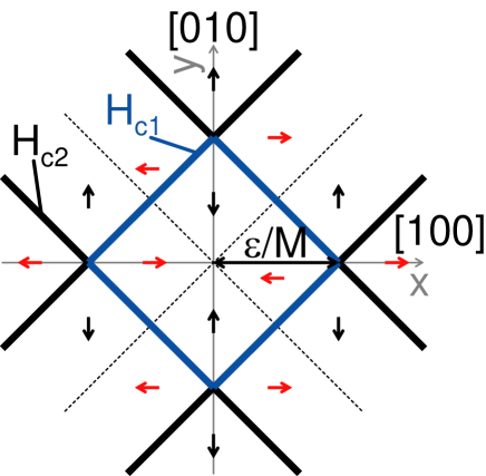
Figure 5: Switching field positions (thick solid lines) in a polar plot for a biaxial material with easy axes along [100] and [010](coordinate axes). The magnetization direction in each region of the plot is indicated by arrows (red/black: high/low resistance) and the hard axes by dashed lines.

We express the switching field positions in this plot (thick lines) in cartesian coordinates using $x=H_{c}\cos\varphi$ and $y=H_{c}\sin\varphi$ to get a better feeling for the switching field behaviour and to extract important parameters.

$$H_{c}\cdot M[\pm\cos\varphi\pm\sin\varphi]$$

(8)

The characteristic polar-plot-pattern for a biaxial material is thus a square with diagonals along the easy axes (the coordinate axes in Fig. 5). The first switching field (thick blue lines) is largest along the easy axes, where H${}_{c1}=\varepsilon/M$. The DW nucleation/propagation energy can be extracted from the diagonal of the square, whose length is equal to $\frac{2\varepsilon_{90^{\circ}}}{M}$. All switching field lines in Fig. 5 have an angle of 45^∘ to the coordinate axes. The dashed lines represent the hard magnetic axes. Arrows illustrate the direction of the magnetization and their color the corresponding resistance state of the respective section in an AMR measurement with current along one of the easy axes.

Neglecting coherent rotation is typically a good model for the first switching fields $H_{c1}$, whereas $H_{c2}$ is influenced by magnetization rotation especially close to the hard axes. Pairs of parallel lines in Fig. 5 do not extend to infinity in practice, they move closer to the hard axes (see the figures and the discussion in section 2.4). The magnetic field needed to force the magnetization parallel to the external field in the hard axis direction is called the anisotropy field $H_{a}$. It is a measure of the anisotropy strength and can be calculated from Eq. 5 using the definition of the anisotropy field: $H_{a}$ is the strength of a field along the hard axis (here 45^∘) needed to suppress the local minima along the easy axes.

$$H_{a}=\frac{2K_{cryst}}{M}$$ (9)

2.1 The Anisotropy Fingerprint Technique

Traditionally the magnetic anisotropy is investigated by direct measurement of the projection of the magnetization onto characteristic directions using SQUID or VSM. The advent of vector field magnets has recently opened up possibilities for acquiring a detailed mapping of the anisotropy. We introduced such a method, which builds on the above discussed angular dependence of the magnetization switching fields, in Ref. [3] and expand upon it here. It is based on summarizing the results of transport measurements into color coded resistance polar plots (RPP) which act as fingerprints for the anisotropy of a given structure. Not only is this method faster than the traditional alternatives, but it is also more sensitive to certain secondary components of the anisotropy, in particular those with easy axes collinear to the primary biaxial anisotropy component[10]. The technique thus often reveals the existence of components which would be missed using standard techniques. Moreover, the technique can be applied to study the anisotropy of layers by using macroscopic transport structures, or applied directly to device elements. It can reveal effects of processing or the influence of small strain fields due to, for example, contacting.

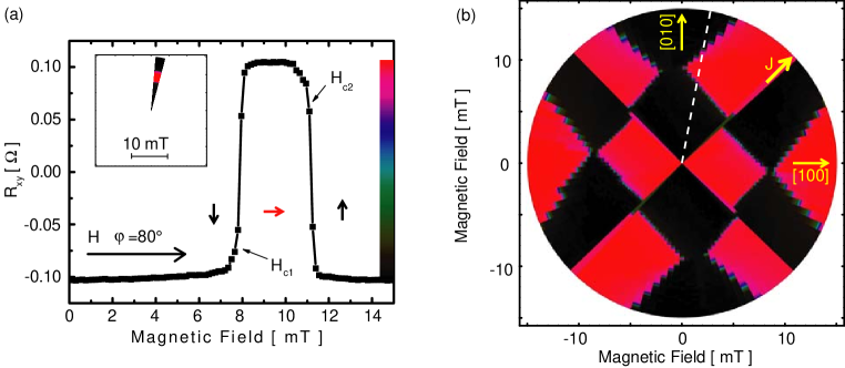
Figure 6: a) Planar Hall Effect measurement along $\varphi=80^{\circ}$ with marked first and second switching field, color scale and the corresponding section of a color coded resistance polar plot(inset). b) Resistance polar plot from a full set of Planar Hall measurements along every $3^{\circ}$. The $80^{\circ}$-section corresponding to (a) is marked by a dashed line.

In the present case the planar Hall effect is used to monitor the magnetization behaviour in a standard Hall bar oriented along the $\langle 110\rangle$ crystal direction. Fig. 6a shows a planar Hall scan along $\varphi=80^{\circ}$. After magnetizing the sample at -300 mT along $80^{\circ}$, the field is brought down to zero. The figure shows the typical double-step switching behaviour as discussed previously in connection with Fig. 3b. The arrows indicate the magnetization direction in the respective field regions with respect to the crystal directions given in Fig. 6b. Abrupt jumps in resistance mark the first and second switching field $H_{c1}$ and $H_{c2}$. The normalized resistance value is color coded according to the scale in Fig. 6a. It is plotted in a polar coordinate system along the magnetic field direction $\varphi$ and with the magnetic field as radial scale. The inset of Fig. 6a shows the polar plot section corresponding to the $80^{\circ}$-scan in this figure. Such Planar Hall scans are recorded along many different in-plane field directions and summarized in the resistance polar plot (RPP) in Fig. 6b. The $80^{\circ}$-segment is marked by a dotted white line.

We can now compare the observed switching field pattern in Fig. 6b with the calculated shape in Fig. 5. While a cursory examination suggests a similar H_c1-pattern, a more detailed comparison reveals significant differences: Focussing on the innermost switching event, the pattern is indeed strongly square-like, confirming that the (Ga,Mn)As has a mainly biaxial magnetic anisotropy at 4 K. The diagonals of this square-like H_c1-pattern are close to the [100] and the [010] crystal direction, the easy axes of the biaxial anisotropy term. However, the inner region is elongated (a rectangle and not a square) - the signature of an additional uniaxial anisotropy term with an easy axis bisecting the biaxial easy axes (Fig. 7c), as will be discussed in section 2.3. Additionally we observe a discontinuity in the middle of the rectangle sides and dark ”open” corners close to the [010] direction. This is characteristic of a uniaxial magnetic anisotropy term collinear with one of the biaxial easy axes (Fig. 7b) and will be discussed in detail in section 2.2.

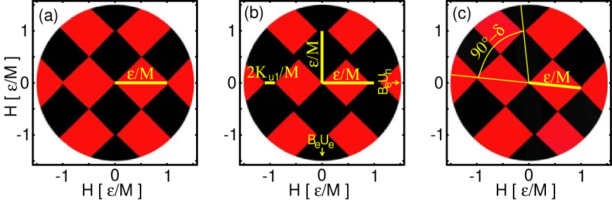
Figure 7: Calculated resistance polar plots for a biaxial material with easy axes along the [100](0^∘) and [010](90^∘) crystal directions(a) and the same material with an additional uniaxial anisotropy along [010](b) or $[1\overline{1}0]$(c). Color scale of the resistance as in Fig. 6. $\varepsilon$ denotes the $90^{\circ}$-DW nucleation/propagation energy.

These qualitative changes in the behaviour of H_c1 are key signatures of the different anisotropy terms of the (Ga,Mn)As layer. A set of high resolution transport measurements compiled into a color coded resistance polar plot thus constitutes a fingerprint of the symmetry components of the anisotropy. It allows for the qualitative and quantitative determination of the different anisotropy terms. It can prove their existence and visualize their respective effects on the magnetization reversal.

2.2 Signature of a $\langle 010\rangle$ Uniaxial Term

The fingerprint of a magnetically biaxial material in Fig. 7a is equivalent to the switching field pattern in Fig. 5. If an additional small uniaxial anisotropy $K_{uni[010]}$ along one of the biaxial easy axes (here along $90^{\circ}$) is present, the square pattern is altered as shown in Fig. 7b. The four-fold symmetry is broken, and the biaxial easy axes correspond to energy minima of slightly different depth, because one of them is parallel (biaxial easy, uniaxial easy; $B_{e}U_{e}$) and one perpendicular (biaxial easy, uniaxial hard; $B_{e}U_{h}$) to the easy axis of the uniaxial anisotropy component.

The angle dependent switching field can be derived as discussed above following [10]: Again it is assumed, that the minima of the energy surface remain at their zero field angles throughout the switching process. In the present case however, the energy minimum along the [010] direction is favored. Its energy is $\Delta E=K_{uni[010]}$ smaller compared with the [100] direction, which results in

$$H_{c}$$

(10)

Magnetization reorientations towards the easier biaxial easy axis $B_{e}U_{e}$ occur now at lower magnetic fields compared to the pure biaxial anisotropy; switches away from $B_{e}U_{e}$ at higher fields. The signs in eq. 10 are chosen appropriately. As a result, the $H_{c1}$- pattern changes as displayed in Fig. 7b. Characteristic features are the steps along the biaxial hard axes, for example along $45^{\circ}$, and the typical ”open corners” along the $B_{e}U_{e}$ axis. These open corners (in black along $90^{\circ}$ in Fig. 7b) arise because a $180^{\circ}$-magnetization reorientation through the nucleation of a $180^{\circ}$-DW is energetically favored in a small angular region around the $B_{e}U_{e}$ axis [10].

Since the isotropic magnetoresistance[11] of typical samples is relatively small compared to the AMR, two magnetization directions differing by $180^{\circ}$ are not distinguishable on the scale considered here, and have nearly the same color in the RPP, creating the characteristic ”open corner”. The strength of the uniaxial anisotropy component can be determined from the separation $\frac{2K_{u1}}{M}$ between $H_{c1}$ and $H_{c2}$ along the $B_{e}U_{h}$ axis.

2.3 Signature of a $\langle\overline{1}10\rangle$ Uniaxial Term

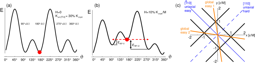
Figure 8: a) A uniaxial $[\overline{1}10]$ anisotropy component flattens the energy surface (eq. 5) and shifts the positions of the energy minima. b) Energy landscape with magnetic field applied along the $-\delta/2$-global easy axis direction. A clockwise and counterclockwise jump of the magnetization (with the respective $\varepsilon$) are equally possible. c) Switching field positions in the polar plot (thick black lines), global easy axes (orange) and easy and hard direction of the $[\overline{1}10]$ anisotropy component (blue).

In this section we describe the effects of a uniaxial anisotropy term $K_{uni[\overline{1}10]}$ with its easy axis (along 135^∘) bisecting the biaxial easy axes. This uniaxial anisotropy component flattens the energy surface (eq. 5) and shifts the positions of the energy minima by (see Fig. 8a)

$$\frac{\delta}{2}=\frac{1}{2}\arcsin(\frac{K_{uni[\overline{1}10]}}{K_{cryst}})$$ (11)

towards the uniaxial easy axis[12]. All four minima have the same energy value. To derive the switching fields we equate the DW nucleation/propagation energy $\varepsilon$ with the difference in Zeeman energy between the initial and final magnetization angle in the respective switching event. As illustrated in Fig. 8a, the magnetization direction can change by 90${}^{\circ}+\delta$ or 90${}^{\circ}-\delta$ depending on whether the magnetization rotates clockwise or counterclockwise. Following [13] we use different DW nucleation/propagation energies $\varepsilon_{90^{\circ}+\delta}$ and $\varepsilon_{90^{\circ}-\delta}$ respectively. The switching field positions in the polar plot given in cartesian coordinates are

$$y_{90^{\circ}+\delta}$$

(12)

Equation 12 describes two parallel sets of lines, as shown in Fig. 8c (thick black lines), whose distance from the origin is determined by the respective $\varepsilon$. MOKE experiments on epitaxial iron films grown on GaAs (with similar anisotropy terms as (Ga,Mn)As) confirm that as expected the sense of the magnetization rotation changes when crossing a global easy axis [12]. The two line sets of eq. 12 represent the clockwise and counterclockwise sense of magnetization rotation. If the field is applied along a global easy axes (minima of Fig. 8a) both rotation directions are energetically equivalent. Consequently the lines must intersect along global easy axes directions. Fig. 8b shows the energy landscape of Fig. 8a when a magnetic field is applied along the $-\delta/2$-global easy axis direction. For both rotation directions, the Zeeman term at the first switching field $H_{c1}$ is equal to the respective $\varepsilon$. We can thus calculate the dependence of $\varepsilon$ on the angle $\Delta\vartheta$ between initial and final magnetization direction:

$$\varepsilon_{90^{\circ}\pm\delta}$$

(13)

which is intuitively reasonable. At the same time we find, that $H_{c1}$ along a global easy axis is $\varepsilon_{90^{\circ}}/M$. Note that this careful treatment of $\varepsilon$ is necessary, the simplified model of a constant $\varepsilon$ independent of the DW angle $\Delta\vartheta$, would lead to the incorrect conclusion, that the rectangle in the polar plot would have its long axis perpendicular to the uniaxial easy direction.

A summary of the above is shown in Fig. 7c. The characteristic pattern of a mainly biaxial anisotropy with a bisecting uniaxial anisotropy component is rectangular. The diagonals of the rectangle are the ”global easy axes”, their length is 2$\varepsilon_{90^{\circ}}/M$. The angle between the global easy axes gives the relative strength of the two anisotropy components (using eq. 11). The easy axis of the uniaxial term is along the median line of the longer edge, for example along 135^∘ in Fig. 7c.

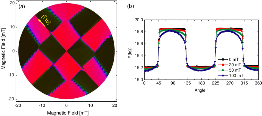
Figure 9: a) Fingerprint of a typical 20 nm thick (Ga,Mn)As Hall bar and b) angle-dependent longitudinal resistance at different fields after magnetizing along $\varphi$.

The presence and sign of the $\langle\overline{1}10\rangle$ anisotropy term can be verified with the help of AMR or PHE measurements at magnetic fields of medium amplitude. For comparison, longitudinal resistance measurements on a Hall bar sample oriented along a (Ga,Mn)As easy axis (0^∘) are converted into the RPP displayed in Fig. 9a. This fingerprint shows an overall biaxial anisotropy with easy axes close to 0^∘ and 90^∘. The central pattern is elongated along 135^∘, suggesting that a uniaxial anisotropy component with easy axis along this direction (the $[\overline{1}10]$ crystal direction) is present.

This is confirmed by the measurements in Fig. 9b. Here the Hall bar sample is first magnetized in a high magnetic field of 300 mT along an angle $\varphi$. The longitudinal resistance is then measured, while the field is slowly stepped down to zero. Fig. 9b shows the resistance values at 100 mT, 50 mT, 20 mT and 0 mT as a function of the field angle. For the interpretation of these curves, imagine for example an energy landscape as shown in Fig. 8, where the strength of the $[\overline{1}10]$ uniaxial anisotropy term is exaggerated. This term describes the width and the height of the ”hills” in the energy surface. The ”hill” in the uniaxial easy axis direction (here 135^∘) is lower than the energy barrier perpendicular to this direction, which is steeper and coincides with the hard magnetic axis of the $[\overline{1}10]$ uniaxial term. At zero field the magnetization is aligned with one of the biaxial easy axes(black curve in Fig. 9b). The steps in this curve mark the peak positions of the ”hills” in the energy landscape - the biaxial hard axes. At medium fields (e.g. 50 mT in Fig. 9b), the magnetization is rotated away from the global easy axes, causing deviations from the step-like behaviour at zero field. These deviations occur at smaller field values along the uniaxial easy direction $[\overline{1}10]$ compared with the uniaxial hard axis [110]. The direction (meaning the sign of $K_{uni[\overline{1}10]}$) of the $[\overline{1}10]$ uniaxial anisotropy is thus the same as in Fig. 9a: the abrupt resistance change at 45^∘ marks the hard and the smoother behaviour at 135^∘ the easy uniaxial axis direction.

2.4 (Ga,Mn)As at 4 K - Typical Fingerprints

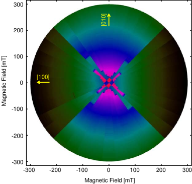
Figure 10: Typical AMR fingerprint measurement of a 100 nm thick (Ga,Mn)As Hall bar. The current direction is along 0^∘.

In the above sections we describe a method which is sensitive enough to detect both, the $[\overline{1}10]$ and the [010] uniaxial anisotropy term. Here we apply the method to our typical (Ga,Mn)As layers and find that all three anisotropy components, the biaxial and the two uniaxial ones, are present in every sample. Various fingerprints show the typical variation of the relative anisotropy terms and the characteristics at low and high fields.

The fingerprints in Figs. 9a, 10 and 11 were compiled from longitudinal AMR measurements on typical (Ga,Mn)As layers of different thickness. All these plots including Fig. 6b show the same general pattern, resembling the four-fold switching field pattern in Fig. 7. The main anisotropy component in all these layers at 4 K is thus biaxial with easy axes along the [100] and [010] direction. The strength of this biaxial term is measured by taking separate high resolution AMR curves along the hard magnetic axes and concluding the anisotropy constant from the anisotropy fields. Typical 2K/M values are of the order of 100 mT…200 mT, as can be seen e.g. in the high field fingerprints in Figs. 10 and  11a and c, where in the sections along the hard axes the magnetization is aligned with the external field at these field values.

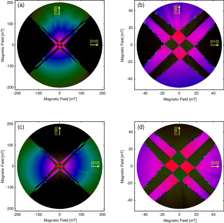
Figure 11: High angular resolution fingerprint measurements (a,b) and close ups of the central region (c,d) for two Hall bars made of the same 70 nm thick material but oriented along orthogonal crystal directions. The current flows along 0^∘ in a and b and along 90^∘ in c and d.

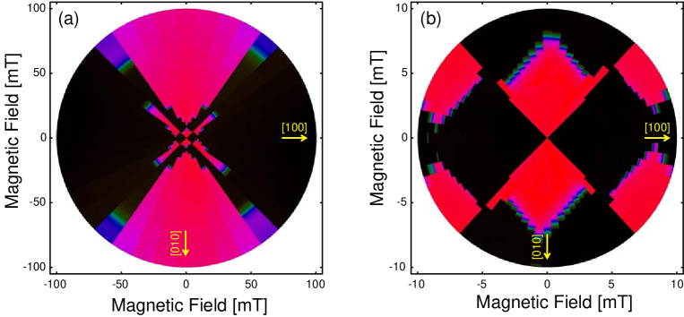
Figure 12: Fingerprint measurement and high resolution RPP at low magnetic field for a 70 nm thick (Ga,Mn)As layer with strongly visible [010] uniaxial anisotropy component but a relatively small $[\overline{1}10]$ term.

The anisotropy components and $\varepsilon$ differ of course from wafer to wafer. The general pattern on the other hand is very similar. All of the RPP show clearly an elongation of the $H_{c1}$-pattern into a rectangle, the signature of the $[\overline{1}10]$ anisotropy component. Steps along the hard axes and the typical open corner are also always present, the typical feature of the [010] anisotropy component. Both uniaxial anisotropy components are thus clearly present in all investigated samples.

The crystal directions are indicated in all fingerprints in yellow. We find, that the elongation of the central pattern, and thus the easy axis of the $[\overline{1}10]$ uniaxial component, points along the $[\overline{1}10]$ crystal direction in all shown typical transport samples. At this point, we would like to note, that the sign of the $[\overline{1}10]$ uniaxial component, i.e. whether the easy axis points along $[\overline{1}10]$ or [110], depends on carrier concentration and Mn doping as shown by [14]. The elongation could thus also be along the [110] direction depending on growth conditions and a possible annealing treatment. In the as grown samples investigated here at 4 K, the typical strength of the $[\overline{1}10]$ uniaxial anisotropy is of the order of 10% of the biaxial anisotropy constant. As examples of the range of values typical for this ratio varies we note a value of 10% from Fig. 12, 15% from Fig. 6b and 20% from Fig. 11.

The open corners of the $H_{c1}$-pattern indicate the direction of the easy axis of the [010] uniaxial term. This easy axis direction is sample dependent and can be along either of the biaxial easy axes of the sample. In the shown polar plots we see this easy axis along [010] in Fig. 6b and along $[100]$ in Figs. 9, 10, 11 and 12. Also the strength of the [010] term is sample dependent. It can dominate the low field switching behaviour as for example in Fig. 12 or be barely visible as in Fig. 9a. In any case, the strength of this anisotropy component is extremely small compared to the main biaxial anisotropy. Even in Fig. 12, where the presence of the [010] uniaxial component has a strong influence on the magnetization behaviour at low fields, its anisotropy field $2K_{uni[010]}/M$ is only 1.6 mT, only 1% of the typical biaxial anisotropy constant.

Figures 11a and c show similar AMR fingerprints on two Hall bars made from the same wafer, but oriented along orthogonal crystal directions. Panels c and d show a close up of the central region. Both fingerprints show virtually the same switching pattern with inverted colors because of the orthogonal current directions. This shows the high homogeneity of the wafer and the robustness of the method. Even on several cool downs, we see virtually the same switching pattern (not shown), although the resistance of the sample changes slightly upon recooling. Note that shape anisotropy in these structures is negligible compared with the crystalline magnetic anisotropy contribution as discussed in Ref. [15]. It is too small to play any significant role in these measurements.

We have neglected coherent rotation to derive simple formulas for the switching fields in the polar plots. This is typically a good model for the first switching fields $H_{c1}$, whereas $H_{c2}$ is influenced by magnetization rotation especially along the hard axes, as mentioned above. The effects of coherent rotation are of course taken into account in the numerical modelling that is based on the energy equation 5.

As discussed previously, the extent of the $H_{c1}$-pattern is determined by $\varepsilon$, while the extent of the $H_{c2}$-features is mainly given by the biaxial anisotropy constant through the anisotropy field (see eq. 9). If the ratio of biaxial anisotropy to $\varepsilon$ is very large, the central pattern is well described by DW-nucleation/propagation-related switching events alone. In the higher field region, the minima of the energy surface move considerably and the $H_{c2}$-switching events approach the hard axes directions.

The typical situation is for example seen in Fig. 10, where AMR curves along every 10^∘ were taken on a Hall bar along 0^∘. The central region shows a rectangular pattern (signature of the $[\overline{1}10]$ uniaxial term) with open corners and steps along the hard axes (signature of the [010] uniaxial term). There is almost no coherent rotation at these low fields. Magnetization reorientations occur through DW nucleation and propagation as seen from the abrupt color changes (between red and blue). The second switching fields along the hard axes (e.g. along 45^∘ at 50 mT) are marked by smooth color transitions proving that coherent rotation is at play. Smooth color transitions at even higher fields (green to black around 0^∘ and red to green around 90^∘) finally are caused by the isotropic MR effect [11].

The fingerprint in Fig. 9 shows a slightly different situation. The ratio of the anisotropy energy to $\varepsilon$ cannot be treated as infinite. For this reason also the $H_{c1}$-pattern shows a considerable influence of coherent rotation. The sides of the rectangle are no longer parallel to each other and the corners do not draw an angle of 90^∘. Still, the elongation is obvious and the difference between switching events towards the two easy axes is observable.

In summary we have shown a variety of fingerprints of typical (Ga,Mn)As transport layers at 4 K. The fingerprint method allowed us to identify the simultaneous presence of the biaxial and two uniaxial anisotropy components. Indeed all (Ga,Mn)As layers investigated show both these uniaxial components, including layers where the [010] component could not be identified in SQUID measurements. As a rule of thumb, the typical relative strength of the anisotropy terms is of the order of $K_{cyst}:K_{uni[\overline{1}10]}:K_{uni[010]}\sim 100:10:1$.

3 Uniaxial Magnetic Anisotropy

This section deals with the magnetization behaviour of magnetically uniaxial materials and how it manifests itself in transport measurements. The latter with two specific applications in mind:

• The (Ga,Mn)As magnetic anisotropy is strongly temperature dependent with the $\langle 110\rangle$ uniaxial anisotropy term being dominant close to the Curie temperature (section 4).

• The fingerprint method can also be used to characterize individual transport structures or even device components. Uniaxial magnetic behaviour was recently achieved by submicron patterning of (Ga,Mn)As and the corresponding anisotropic strain relaxation [15].

We again track the magnetization angle using AMR measurements and finally discuss the color-coded RPP, the anisotropy fingerprint, expected for a material with uniaxial magnetic anisotropy.

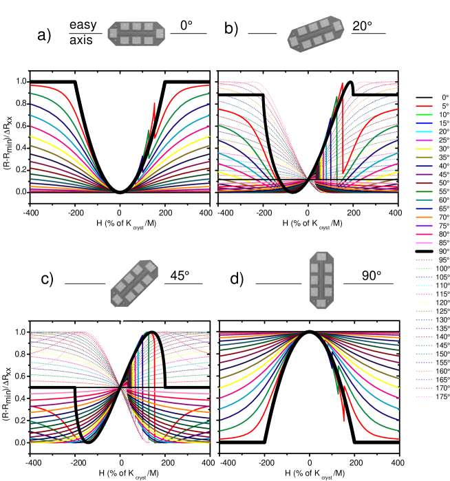
Figure 13: Calculated anisotropic magnetoresistance curves in a magnetically uniaxial material for magnetic field sweeps along many in-plane directions($0^{\circ}..85^{\circ}$ thin solid, $90^{\circ}$ thick, $95^{\circ}..175^{\circ}$ dashed) for Hall bar orientations as in the sketches with current along (a) $0^{\circ}$ , (b) $20^{\circ}$, (c) $45^{\circ}$, and (d) $90^{\circ}$. All angles with respect to the uniaxial easy axis. The field is swept from left to right.

Fig. 13 shows AMR curves calculated for a magnetically uniaxial material using Eq. 5 with $\varepsilon$ =30% $K_{uni}$. The individual panels illustrate how the current direction with respect to the easy axis modifies the overall picture of a set of AMR curves. In all four panels a single zero field resistance state can be identified, corresponding to the easy axis magnetization orientation. The resistance value is given by the angle between current and easy axis through Eq. 2. If the external field is swept along this easy axis direction ($0^{\circ}$, thin black line), the magnetization is aligned with the easy axis throughout the whole scan, yielding a horizontal line through the focal point at zero field. The hard axis scan (thick line) reveals the anisotropy field; (the same as in the biaxial case, Eq. 9)

$$H_{a}=\frac{2K_{uni}}{M}$$ (14)

the external magnetic field perpendicular to the easy axis, where the magnetization starts to deviate from the field direction. The magnetization rotation in panels (a) and (d) yields a parabolic dependence of the resistance on the field amplitude [16]. In all other MR scans the magnetization relaxes to the closest easy axis direction while the field is decreased from high negative values, reaching the focal point at zero field. After zero, the magnetization direction reverses by circa $180^{\circ}$ through DW nucleation and propagation, which is visible as abrupt resistance changes in Fig. 13, for example the spikes around 100% K_uni in panel (a). A back sweep results in a hysteretically symmetric curve with the switching events at negative fields (not shown).

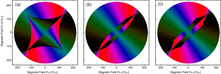
Figure 14: Calculated AMR fingerprints of a magnetically uniaxial material with easy axis along $135^{\circ}$ and current along $0^{\circ}$. Magnetization reversal through (a) coherent rotation only (Stoner-astroid) and (b) DW nucleation and propagation with $\varepsilon$ according to Eq. 13 (c) simplified model assuming a constant $\varepsilon=2\varepsilon_{90^{\circ}}$. ($\varepsilon_{90^{\circ}}$ =30% $K_{uni}$)

Fig. 14 shows the results of similar calculations with high angular resolution plotted in RPP fashion. Here the easy axis is oriented along $135^{\circ}$ and the current flow along $0^{\circ}$. The colors are a function of the the current direction, for example dark color at high magnetic fields along the current, while the switching event pattern is defined by the magnetic properties alone.

If a structure is smaller than the single-domain limit [17, 18] it is energetically unfavourable to nucleate a DW. Instead the magnetization rotates coherently (Stoner-Wohlfarth model  [8]). Fig. 14a shows the well known Stoner-Wohlfarth astroid [8, 19] which describes the switching positions of a uniaxial particle under coherent rotation. Its extent in both the easy and the hard axis direction is given by the anisotropy field.

Allowing for DW nucleation with $\varepsilon$ according to eq. 13 truncates the easy axis corners of the astroid as shown in Fig. 14b. The extent $\varepsilon_{90^{\circ}}/M$ in the easy axis direction is a measure for the DW nucleation/propagation energy. A field sweep along the hard magnetic axis, is still fully described by Stoner-Wohlfarth rotation and the extent in this direction is given by the anisotropy field. The detailed shape of the switching field pattern depends on the model used for the $\varepsilon$-dependence on the DW angle. Fig. 14c shows the RPP calculated assuming a constant $\varepsilon_{\Delta\vartheta}=2\varepsilon_{90^{\circ}}$ independent of the magnetization directions of the domains separated by the DW. While the easy and hard axis extent are the same as in Fig. 14b, the better correspondence of the shape of the features in (b) then (c) to the experimental data is further evidence in support for the above described description of the DW energies.

4 Temperature Dependence of the (Ga,Mn)As Anisotropy

The fingerprint method provides us with the opportunity to investigate the temperature dependence of the magnetic anisotropy. Figures 15 and 16 show AMR fingerprints at various temperatures for the layer investigated in Fig. 11 at 4.2 K. The left column shows results on a Hall bar patterned along 90^∘ (the [100] crystal direction). In the right column the Hall bar is oriented along 0^∘. The layer is, as typical, very homogeneous and the switching patterns in the two columns are virtually identical at all temperatures (except for a trivial inversion of the color scales).

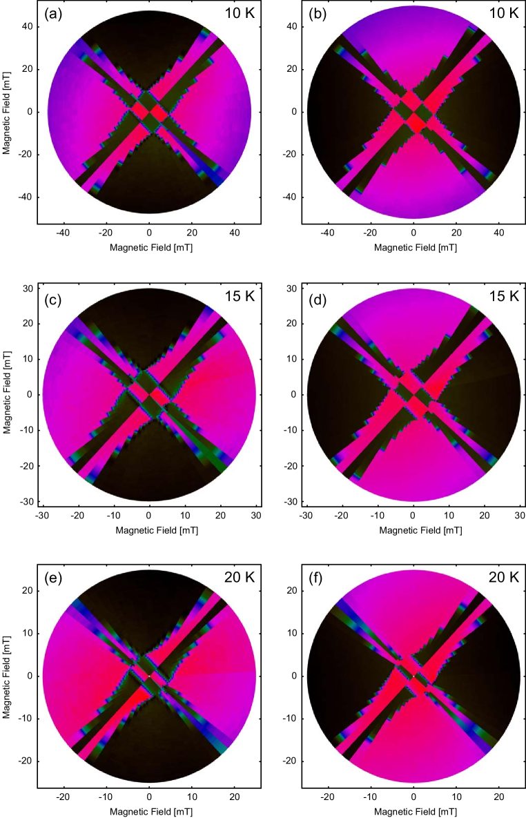
Figure 15: Temperature dependent AMR fingerprint measurements of the sample in Fig. 11a and b (right column) with current along 0^∘ and Fig. 11c and d (left column) with current along 90^∘.

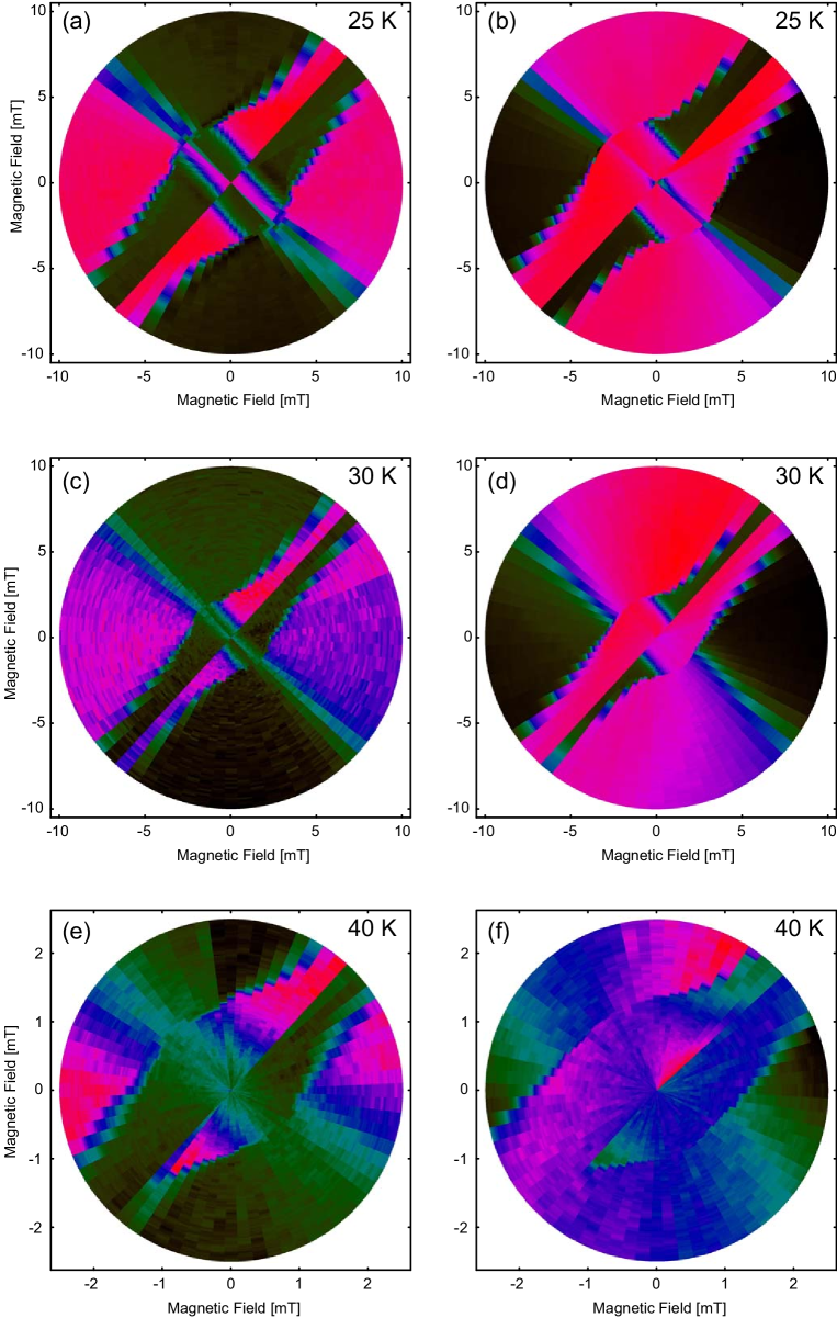
Figure 16: High temperature AMR fingerprint measurements, continuation of Fig. 15.

The mainly biaxial anisotropy is the origin of the nearly four-fold symmetry in the low temperature fingerprints. The uniaxial anisotropy term with easy axis along the $[\overline{1}10]$ crystal direction takes over with increasing temperature and becomes the dominant term close to T_C: already the fingerprints at 30 K exhibit the typical 2-fold symmetry of a uniaxial anisotropy. The short axis of the pattern marks the uniaxial easy axis; the extended feature perpendicular to it the magnetic hard axis (see Sec. 3 for details). The AMR amplitude and the switching fields, i.e. the size of the fingerprint pattern, decrease significantly with temperature (note the different magnetic field scales).

This is consistent with detailed SQUID studies [2, 20]. There the anisotropy constants $K_{cryst}$ and $K_{[\overline{1}10]}$ were extracted from hard axis magnetization measurements vs magnetic field. The two terms exhibited different temperature dependence. In particular it was observed that the temperature dependence of the anisotropy constants originates in their power-law dependence on the volume magnetization $M$. While the uniaxial anisotropy constant is proportional to the square of $M$, the biaxial term depends on $M^{4}$. As a result, the biaxial anisotropy term, which dominates the magnetic behaviour at 4 K, decreases much faster with increasing temperature than the uniaxial term. This is the reason why the magnetic anisotropy undergoes a transition from mainly biaxial to mainly uniaxial when the temperature increases from 4 K to T_C.

Fig. 17a shows SQUID measurements on the sample of Figs. 15 and 16. After magnetizing the sample along a given direction, we measure the projection of the remanent magnetization on the respective axis and its evolution with increasing temperature. Displayed are measurements along the two 4 K hard magnetic axes [110] and $[\overline{1}10]$ and one of the biaxial easy axes $\langle 010\rangle$. They show the same anisotropy transition as the fingerprints above. At 4 K, the $\langle 010\rangle$ crystal direction is close to a global magnetic easy axis and thus shows the largest projection of the remanent magnetic moment. The $[\overline{1}10]$ direction coincides with the easy axis of the uniaxial K${}_{uni[\overline{1}10]}$ anisotropy term. That is why it is closer to a global easy axis than the [110] direction [21] and in consequence shows a larger projection of the remanent moment. As temperature increases, the magnetization decreases and the relative amplitude of the anisotropy terms changes, as described above. This results in a gradual reorientation of the global easy axes with temperature, changing the angle between remanent magnetization (along the global easy axis closest to the sweep direction in Fig. 17a) and the respective sweep direction. The result of both the decreasing volume magnetization and changing relative projections onto the different sweep directions, can be seen in Fig. 17a. The green $[\overline{1}10]$ remanence, e.g., gains relative weight with increasing temperature. This supports the observations of the fingerprint measurements, where the $[\overline{1}10]$ anisotropy term gains in influence at higher temperatures. Given the specific anisotropy behaviour, known from the transport measurements, we can estimate the absolute value of the remanent magnetization from the square root of the sum of the squares of the two magnetization projections along $[\overline{1}10]$ and [110](Pythagorean theorem) [2]. The result is displayed in gray in Fig. 17a. Such a magnetization measurement with SQUID is complementary to transport investigations, since those can only give energy scales in field units, i.e. normalized to the volume magnetization like K/$M$ or $\varepsilon$/$M$.

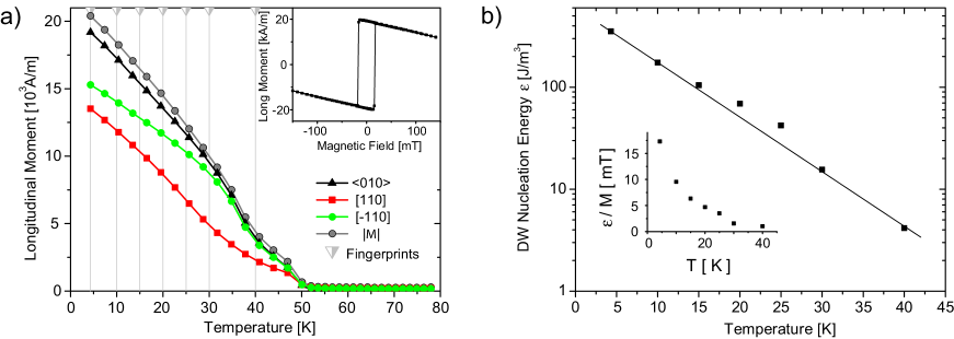
Figure 17: a) Measurement of the projection of the remanent magnetic moment of the sample of Figs. 15 and 16 onto different crystal axes by SQUID magnetometry. Vertical gray lines indicate the temperatures of the fingerprint measurements in Figs. 15 and 16. b) Domain wall nucleation energy $\varepsilon_{90^{\circ}}$ (symbols) versus temperature, derived from $\varepsilon_{90^{\circ}}/M$ (inset) extracted from the fingerprints.

The quantitative determination of the anisotropy constants at higher temperatures is more complex than at 4 K and work is ongoing to find a set of straightforward rules as for the mainly biaxial system at 4 K. Determining the domain wall nucleation/propagation energy $\varepsilon$, however, is possible with the described techniques. Black symbols in Fig. 17b show preliminary results determined from the fingerprints in Figs. 15 and  16. The line is a guide to the eye. The method for the extraction builds on the techniques described in section 2: 2$\varepsilon$/$M$ is basically given by the diagonal of the rectangular first switching field pattern for mainly biaxial samples and by the easy axis direction diameter for purely uniaxial samples. The strength of this method is that we can extract $\varepsilon_{90^{\circ}}$ easily from the plots, because the global easy axes directions are obvious from symmetry considerations. It is not necessary to assume a constant (or known) global easy axis direction and we can thus fully account for the complex temperature dependence of the easy axis behaviour without fitting the data to a complicated model. Both the determination of M and of $\varepsilon$/$M$ are not as accurate in the transition region, where the energy surface at zero field is almost flat over a wide angular range. This is a probable cause of the deviation from perfect exponential behaviour for the data in Fig. 17b at intermediate temperatures.

The square hysteresis loop with abrupt switching events, shown in the inset of Fig. 17a, points to a DW nucleation dominated process, as opposed to a process, where the energy needed for DW propagation is the limiting parameter [22]. Also the temperature dependence of the DW nucleation energy in Fig. 17b fits to the standard exponential behaviour expected for the temperature dependence of the coercivity [23, 24]. We suggest that the above method is one tool that, in combination with, e.g., time dependent and optical investigations [25], can clarify the DW nucleation process in (Ga,Mn)As. It can complement recent optical studies, that identify the nature of pinning centers and visualize the process of DW-related magnetization switching in (Ga,Mn)As [26, 27].

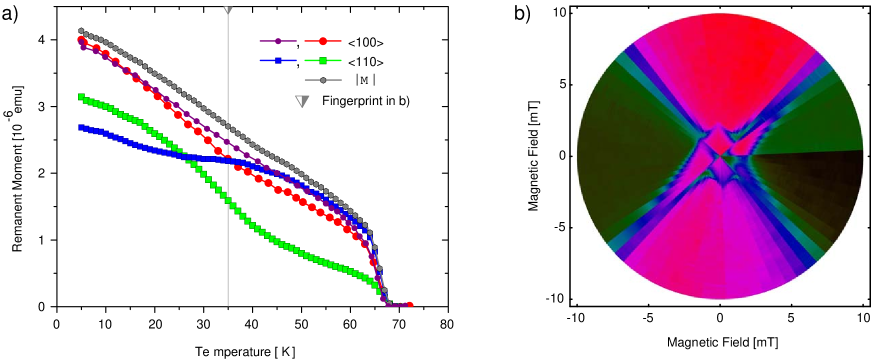
Figure 18: a) Projection of the remanent magnetic moment of a 20 nm thick (Ga,Mn)As layer measured with SQUID along different crystal axes. 35 K, the temperature of the anisotropy fingerprint measurement [28] in b) is indicated by a vertical gray line.

SQUID studies on another sample are shown in Fig. 18a. As in Fig. 17a we plot the projection of the remanent magnetic moment vs temperature. Shown are measurements along the two biaxial easy axes (red and purple) and along the two bisecting directions (green and blue). The absolute value of the volume magnetization is estimated as discussed above (gray). The large difference between the two biaxial easy axes directions (red and purple) at intermediate temperatures (25 to 60 K) points to a symmetry breaking caused by a relatively strong uniaxial [010] anisotropy component. For this reason we investigate this sample at 35 K, where the [010] component should be strongly visible in the symmetry of the fingerprint pattern, and where the transport signal is still large enough to get clean measurements. Fig. 18b shows the resulting fingerprint. The symmetry breaking between the two biaxial easy axes (here along 0^∘ and 90^∘) is apparent from the picture. The relatively strong uniaxial [010] term causes a preference for the magnetization orientation along $90^{\circ}$. The resistance polar plot in turn resembles in parts a typical biaxial fingerprint pattern (between 45^∘ and 135^∘ and the point symmetric region) and in the other quadrants a typical uniaxial fingerprint pattern (between 135^∘ and 225^∘).[28] We can thus conclude, that the relatively small uniaxial term gains in importance at intermediate temperatures in this sample. This is where the two stronger anisotropy terms have approximately equal weight, compensating each other in specific angular regions. A small extra term in the energy equation then plays a huge role: it creates an additional local minimum in the energy surface, causing very different switching behaviour in different quadrants of the polar plot.

In summary, we have shown that the extended anisotropy fingerprint technique is a powerful method to access the fine details of complex anisotropies in ferromagnetic semiconductors. We used this method to show that all transport layers investigated showed three symmetry components of the magnetic anisotropy; the main biaxial term and two uniaxial terms along the $[\overline{1}10]$ and the [010] crystal directions. The relative strength of these anisotropy terms is roughly speaking, of the order of $K_{cyst}:K_{uni[\overline{1}10]}:K_{uni[010]}\sim 100:10:1$ at 4 K. At higher temperatures the relative strength of the $[\overline{1}10]$ anisotropy component increases. The overall behaviour of the anisotropy terms is consistent with SQUID investigations, showing the typical transition from a mainly biaxial to a mainly uniaxial material with increasing temperature. An extraction of the 90^∘-DW nucleation energy and its temperature dependence is also possible. Measurements have shown, that the [010] uniaxial anisotropy term, whose existence is sometimes questioned, can be clearly observed. We show that it can have a particularly strong impact on the switching behaviour for cases where the cooperative effect of the biaxial and the $[\overline{1}10]$ uniaxial anisotropy term lead to a flattened energy surface.

References

References

- [1] X. Liu and J. K. Furdyna, J. Phys. Condens. Matter 18, R245 R279 (2006)
- [2] K.Y Wang, M. Sawicki, K.W. Edmonds, R.P. Campion, S. Maat, C.T. Foxon, B.L. Gallagher, and T. Dietl. Phys. Rev Lett., 95:217204, 2005.
- [3] K. Pappert, S. Hümpfner, J. Wenisch, K. Brunner, C. Gould, G. Schmidt, and L. Molenkamp. Appl. Phys. Lett., Vol. 90, p. 062109, 2007.
- [4] D. V. Baxter, D. Ruzmetov, J. Scherschligt, Y. Sasaki, X. Liu, J. K. Furdyna, and C. H. Mielke.Phys. Rev. B, Vol. 65, p. 212407, 2002.
- [5] J. P. Jan. (Eds: F. Seitz, D. Turnbull), Academic Press Inc. New York, 1957.
- [6] T. R. McGuire and R. I. Potter. IEEE Trans. Magn., Vol. MAG-11, p. 1018, 1975.
- [7] C. Gould, C. Rüster, T. Jungwirth, E. Girgis, G.M. Schott, R. Giraud, K. Brunner, G. Schmidt, and L.W. Molenkamp. Phys. Rev. Lett., 93:117203, 2004.
- [8] E.C. Stoner and E.P. Wohlfarth. Phil. Trans. Roy. Soc. A, 240:599, 1948.
- [9] R.P. Cowburn, S.J. Gray, and J.A.C. Bland. Phys. Rev. Lett., 79:4018, 1997.
- [10] R.P. Cowburn, S. Gray, J. Ferré, J. Bland, and J. Miltat. J. Appl. Phys., 78:7210, 1995.
- [11] F. Matsukura, M. Sawicki, T. Dietl, D. Chiba, and H. Ohno. Physica E, Vol. 21, p. 1032, 2004.
- [12] C. Daboo, R. J. Hicken, D. E. P. Eley, M. Gester, S. J. Gray, A. J. R. Ives, and J. A. C. Bland. J. Appl. Phys., 75:5586, 1994.
- [13] H. X. Tang, R. K. Kawakami, D. D. Awschalom, and M. L. Roukes. Phys. Rev. Lett., 90:107201, 2003.
- [14] M. Sawicki, K.-Y. Wang, K. W. Edmonds, R. P. Campion, C. R. Staddon, N. R. S. Farley, C. T. Foxon, E. Papis, E. Kaminska, A. Piotrowska, T. Dietl, and B. L. Gallagher, Phys. Rev. B 71, 121302(R) (2005) (4 pages)
- [15] S. Hümpfner, K. Pappert, J. Wenisch, K. Brunner, C. Gould, G. Schmidt, and L.W. Molenkamp, Appl. Phys. Lett. 90 102102 (2007).
- [16] F.G. West. Nature, 188:129, 1960.
- [17] W.F. Brown. J. Appl.Phys., 39:993, 1968.
- [18] A. Aharoni. J. Appl. Phys., 63:5879, 1988.
- [19] A. Hubert and R. Schäfer. Springer, Heidelberg, 2000.
- [20] M. Sawicki, K. Y. Wang, K.W. Edmonds, R.P. Campion, C.R. Staddon, N.R.S. Farley, C.T. Foxon, E. Papis, E. Kamiska, A. Piotrowska, T. Dietl, and B.L. Gallagher. Phys. Rev. B, 71:R121302, 2005.
- [21] See Fig. 8, where [110] is along and along .
- [22] J. Ferré. Spin Dynamics in Confined Magnetic Structures I, pages 127–165. (Eds: . Hillebrands and K. Ounadjela), Springer, 2002.
- [23] The extraction method already accounts for the correction of the temperature dependence of the anisotropy and the understanding of the respective fingerprint pattern guaranties that only switching events due to DW nucleation are analyzed, as distinct from switching events that are caused by Stoner-Wohlfarth rotation. The ”constant anisotropy” criterion for the exponential behaviour is thus satisfied.
- [24] Vertesy and Tomas. J. Appl. Phys., 77:6425, 1995.
- [25] L. Thevenard, L. Largeau, O. Mauguin, G. Patriarche, and A. Lemaître, N. Vernier and J. Ferré, Phys. Rev. B 73, 195331 (2006).
- [26] K. Y. Wang, A. W. Rushforth, V. A. Grant, R. P. Campion, K. W. Edmonds, C. R. Staddon, C. T. Foxon, B. L. Gallagher, J. Wunderlich, and D. A. Williams. to be published in J. Appl. Phys.; arXiv:0705.0474 2007.
- [27] A. Dourlat, C. Gourdon, V. Jeudy, C. Testelin, L. Thevenard, and A. Lemaître, phys. stat. sol. (c) 3, 4074 4077 (2006).
- [28] The small resistance deviation of % in the last quadrant is caused by temperature drift. The temperature decreased by during the measurement between and , changing the relative weight of the biaxial and the uniaxial anisotropy components, slightly modifying the fingerprint pattern in this section.