Optimal experimental design
and some related control problems

Abstract

This paper traces the strong relations between experimental design and control, such as the use of optimal inputs to obtain precise parameter estimation in dynamical systems and the introduction of suitably designed perturbations in adaptive control. The mathematical background of optimal experimental design is briefly presented, and the role of experimental design in the asymptotic properties of estimators is emphasized. Although most of the paper concerns parametric models, some results are also presented for statistical learning and prediction with nonparametric models.

,

1 Introduction

The design of experiments (DOE) is a well developed methodology in statistics, to which several books have been dedicated, see e.g. [42], [167], [125], [4], [149], [44]. See also the series of proceedings of the Model-Oriented Design and Analysis workshops (Springer Verlag 1987; Physica Verlag, 1990, 1992, 1995, 1998, 2001, 2004). Its application to the construction of persistently exciting inputs for dynamical systems is well known in control theory (see Chapter 6 of [58], Chapter 14 of [104], Chapter 6 of [188], the book [196] and the recent surveys [53], [66]). A first objective of this paper is to briefly present the mathematical background of the methodology and make it accessible to a wider audience. DOE, which can can be apprehended as a technique for extracting the most useful information from data to be collected, is thus a central (and sometimes hidden) methodology in every occasion where unknown quantities must be estimated and the choice of a method for this estimation is open. DOE may therefore serve different purposes and happens to be a suitable vehicle for establishing links between problems like optimization, estimation, prediction and control. Hence, a second objective of the paper is to exhibit links and similarities between seemingly different issues (for instance, we shall see that parameter estimation and prediction of a model response are essentially equivalent problems for parametric models and that the construction of an optimal method for global optimization can be casted as a stochastic control problem). At the same time, attention will be drawn to fundamental differences that exist between seemingly similar problems (in particular, evidence will be given of the gap between using parametric or nonparametric models for prediction). A third objective is to point out and explain some inherent difficulties in estimation problems when combined with optimization or control (hence we shall see why adaptive control is an intrinsically difficult subject), indicate some tentative remedies and suggest possible developments.

Mentioning these three objectives should not shroud the main message of the paper, which consists in pointing out prospective research directions for experimental design in relation with control, in short: classical DOE relies on the assumption of persistence of excitation but many issues remain open in other situations; DOE should be driven by the final purpose of the identification (the intended model application of [57]) and this should be reflected in the construction of design criteria; DOE should face the new challenges raised by nonparametric models and robust control; algorithms and practical methods for DOE in non-standard situations are still missing. The program is rather ambitious, and this survey does not pretend to be exhaustive (for instance, only the case of scalar observations is considered; Bayesian techniques are only slightly touched; measurement errors are assumed to be independent, although correlated errors would deserve a special treatment; distributed parameter systems are not considered; nonparametric modelling is briefly considered and for static systems only, etc.). However, references are indicated where a detailed enough presentation is lacking. None of the results presented is really new, but their collection in a single document probably is, and will hopefully be useful to the reader.

Section 2 presents different types of application of optimal experimental design, partly through examples, and serves as an introduction to the topic. In particular, the fourth application concerns optimization and forms a preliminary illustration of the link between sequential design and adaptive control. Section 3 concerns statistical learning and nonparametric modelling, where DOE is still at an early stage of development. The rest of the paper mainly deals with parametric models, for which parameter uncertainty is suitably characterized through information matrices, due to the asymptotic normality of parameter estimators and the Cramér-Rao bound. This is considered in Section 4 for regression models. Section 5 presents the mathematical background of optimal experimental design for parameter estimation. The case of dynamical models is considered in Section 6, where the input is designed to yield the most accurate estimation of the model parameters, while possibly taking a robust-control objective into account. Section 7 concerns adaptive control: the ultimate objective is process control, but the construction of the controller requires the estimation of the model parameters. The difficulties are illustrated through a series of simple examples. Optimal DOE yields input sequences that are optimally (and persistently) exciting. At the same time, by focussing attention on parameter estimation, it reveals the intrinsic difficulties of adaptive control through the links between dual (active) control and sequential design. General sequential design (for static systems) is briefly considered in Section 8. Finally, Section 9 suggests further developments and research directions in DOE, concerning in particular active learning and nonlinear feedback control. Here also the presentation is mainly through examples.

2 Examples of applications of DOE

Although the paper is mainly dedicated to parameter estimation issues, DOE may have quite different objectives (and it is indeed one of the purposes of the paper to use DOE to exhibit links relating these objectives). They are illustrated through examples which also serve to progressively introduce the notations. The first one concerns an extremely simple parameter estimation problem where the benefit of a suitably designed experiment is spectacular.

2.1 A weighing problem

Suppose we wish to determine the weights of eight objects with a chemical balance. The result $y$ of a weighing (the observation) corresponds to the mass on the left pan of the balance minus the mass on the right pan plus some measurement error $\varepsilon$. The errors associated with a series of measurements are assumed to be independently identically distributed (i.i.d.) with the normal distribution ${\mathcal{N}}(0,\sigma^{2})$. The objects have weights $\bar{\theta}_{i}$, $i=1,\ldots,8$. Each weighing is characterized by a 8-dimensional vector ${\bf u}$ with components $\{{\bf u}\}_{i}$ equal to $1$, $-1$ or $0$ depending whether object $i$ is on the left pan, the right pan or is absent from the weighing, and the associated observation is $y={\bf u}^{\top}\mbox{\boldmath$\bar{\theta}$}+\varepsilon$. We thus have a linear model (in the statistical sense: the response is linear in the parameter vector $\theta$), and the Least-Squares (LS) estimator $\mbox{\boldmath$\hat{\theta}$}^{N}$ associated with $N$ observations $y_{k}$ characterized by experimental conditions (design points) ${\bf u}_{k}$, $k=1,\ldots,N$, is

$$\mbox{\boldmath$\hat{\theta}$}^{N}=\arg\min_{\mbox{\boldmath$\theta$}}\sum_{k=1}^{N}[y_{k}-{\bf u}_{k}^{\top}{\mbox{\boldmath$\theta$}}]^{2}={\bf M}_{N}^{-1}\sum_{k=1}^{N}y_{k}{\bf u}_{k}\,,$$ (1)

$$\mbox{with }{\bf M}_{N}=\sum_{k=1}^{N}{\bf u}_{k}{\bf u}_{k}^{\top}\,.$$ (2)

We consider two weighing methods. In method $a$ the eight objets are weighed successively: the vectors ${\bf u}_{i}$ for the eight observations coincide with the basis vectors ${\bf e}_{i}$ of $\mathbb{R}^{8}$ and the observations are $y_{i}=\bar{\theta}_{i}+\varepsilon_{i}$, $i=1,\ldots,8$. The estimated weights are simply given by the observations, that is, $\hat{\theta}_{i}=y_{i}\sim{\mathcal{N}}(\bar{\theta}_{i},\sigma^{2})$. Method $b$ is slightly more sophisticated. Eight measurements are performed, each time using a different configuration of the objets on the two pans so that the vectors ${\bf u}_{i}$ form a $8\times 8$ Hadamard matrix ($|\{{\bf u}_{i}\}_{j}|=1$ $\forall i,j$ and ${\bf u}_{i}^{\top}{\bf u}_{j}=0$ $\forall i\neq j$, $i,j=1,\ldots,8$). The estimates then satisfy $\hat{\theta}_{i}\sim{\mathcal{N}}(\bar{\theta}_{i},\sigma^{2}/8)$ with 8 observations only. To obtain the same precision with method $a$, one would need to perform eight independent repetitions of the experiment, requiring 64 observations in total.

In a linear model of this type, the LS estimator (1) is unbiased: ${\rm I}\!{\rm E}_{\theta}\{\mbox{\boldmath$\hat{\theta}$}^{N}\}-{\mbox{\boldmath$\theta$}}=0$, where ${\rm I}\!{\rm E}_{\theta}\{\cdot\}$ denotes the mathematical expectation conditionally to $\theta$ being the true vector of unknown parameters. Its covariance matrix is ${\rm I}\!{\rm E}_{\theta}\{(\mbox{\boldmath$\hat{\theta}$}^{N}-{\mbox{\boldmath$\theta$}})(\mbox{\boldmath$\hat{\theta}$}^{N}-{\mbox{\boldmath$\theta$}})^{\top}\}=\sigma^{2}{\bf M}_{N}^{-1}$ with ${\bf M}_{N}$ given by (2) (note that it does not depend on $\theta$). Choosing an experiment that provides a precise estimation of the parameters thus amounts to choosing $N$ vectors ${\bf u}_{k}$ such that (${\bf M}_{N}$ is non singular and) “${\bf M}_{N}^{-1}$ is as small as possible”, in the sense that a scalar function of ${\bf M}_{N}^{-1}$ is minimized (or a scalar function of ${\bf M}_{N}$ is maximized), see Section 5. In the weighing problem above the optimization problem is combinatorial since $\{{\bf u}_{k}\}_{i}\in\{-1,0,1\}$. In the design of method $b$ the vectors ${\bf u}_{k}$ optimize most “reasonable” criteria $\Phi({\bf M}_{N})$, see, e.g., [29], [162]. This case will not be considered in the rest of the paper but corresponds to a topic that has a long and rich history (it originated in agriculture through the pioneering work of Fisher, see [46]).

2.2 An example of parameter estimation in a dynamical model

The example is taken from [39] and concerns a so-called compartment model, widely used in pharmacokinetics. A drug $x$ is injected in blood (intravenous infusion) with an input profile $u(t)$, the drug moves from the central compartment $C$ (blood) to the peripheral compartment $P$, where the respective quantities of drugs at time $t$ are denoted $x_{C}(t)$ and $x_{P}(t)$. These obey the following differential equations:

$$\left\{\begin{array}[]{rcllcl}\frac{dx_{C}(t)}{dt}&=&(-K_{EL}-&K_{CP})x_{C}(t)&+&K_{PC}x_{P}(t)+u(t)\\ \frac{dx_{P}(t)}{dt}&=&&K_{CP}x_{C}(t)&-&K_{PC}x_{P}(t)\\ \end{array}\right.$$

where $K_{CP}$, $K_{PC}$ and $K_{EL}$ are unknown parameters. One observes the drug concentration in blood, that is, $y(t)=x_{C}(t)/V+\varepsilon(t)$ at time $t$, where the errors $\varepsilon(t_{i})$ corresponding to different observations are assumed to be i.i.d. ${\mathcal{N}}(0,\sigma^{2})$ and where $V$ denotes the (unknown) volume of the central compartment. There are thus four unknown parameters to be estimated, which we denote $\mbox{\boldmath$\theta$}=(K_{CP},K_{PC},K_{EL},V)$. The profile of the input $u(t)$ is imposed: it consists of a 1 min loading infusion of 75 mg/min followed by a continuous maintenance infusion of 1.45 mg/min. The experimental variables correspond to the sampling times $t_{i}$, $1\leq t_{i}\leq 720\mbox{ min}$ (the time instants at which the observations — blood samples — are taken). Suppose that the true parameters take the values $\mbox{\boldmath$\bar{\theta}$}=(0.066\,\mbox{min}^{-1},\ 0.038\,\mbox{min}^{-1},\ 0.0242\,\mbox{min}^{-1},\ 30\,\mbox{l)}$. Two different experimental designs are considered. The first one, called “conventional”, is given by ${\bf t}=(5,10,30,60,120,180,360,720)\mbox{ (in min)}$; the “optimal” one ($D$-optimal for $\bar{\theta}$, see Section 5.1) is ${\bf t}^{*}=(1,1,10,10,74,74,720,720)\mbox{ (in min)}$. (Note that both designs contain 8 observations and that ${\bf t}^{*}$ comprises repetitions of observations at the same time — which means that it is implicitly assumed that the collection of several simultaneous independent measurements is possible.) Figure 1 presents the (approximate) marginal density for the LS estimator of $K_{EL}$, see [129], [139], when $\sigma=0.2\mu\mbox{g/ml}$. Similar pictures are obtained for the other parameters.

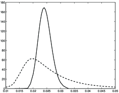
Figure 1: Approximate marginal densities for the LS estimator $\hat{K}_{EL}$ (dashed line for the conventional design, solid line for the optimal one); the true value is $\bar{K}_{EL}=0.0242\mbox{ min}^{-1}$.

Clearly, the “optimal” design ${\bf t}^{*}$ yields a much more precise estimation of $\theta$ than the conventional one, although both involve the same number of observations. On the other hand, with $4=\dim(\mbox{\boldmath$\theta$})$ sampling times only, ${\bf t}^{*}$ does not permit to test the validity of the model. DOE for model discrimination, which we consider next, is especially indicated for situations where one hesitates between several structures.

2.3 Discrimination between model structures

Design for discrimination between model structures will not be detailed in the paper, only the basic principle of a simple method is indicated below and one can refer to [17] and the survey papers [3], [65] for other approaches. When there are two model structures $\eta^{(1)}(\mbox{\boldmath$\theta$}_{1},{\bf u})$ and $\eta^{(2)}(\mbox{\boldmath$\theta$}_{2},{\bf u})$ and the errors are i.i.d., a simple sequential procedure is as follows, see [5]:
$\bullet$ after the observation of $y({\bf u}_{1}),\ldots,y({\bf u}_{k})$ estimate $\mbox{\boldmath$\hat{\theta}$}_{1}^{k}$ and $\mbox{\boldmath$\hat{\theta}$}_{2}^{k}$ for both models;
$\bullet$ place next point ${\bf u}_{k+1}$ where $[\eta^{(1)}(\mbox{\boldmath$\hat{\theta}$}_{1}^{k},{\bf u})-\eta^{(2)}(\mbox{\boldmath$\hat{\theta}$}_{2}^{k},{\bf u})]^{2}$ is maximum;
$\bullet$ $k\rightarrow k+1$, repeat.
When there are more than two structures in competition, one should estimate $\mbox{\boldmath$\hat{\theta}$}_{i}^{k}$ for all of them and place the next point using the two models with the best and second best fitting, see [6]. The idea is to place the design point where the predictions of the competitors differ much, so that when one of the structures is correct (which is the underlying assumption), next observation should be close to the prediction of that model and should thus give evidence that the other structures are wrong. Similar ideas can be used to design input sequences for detecting changes in the behavior of dynamical systems, see the book [82].

2.4 Optimization of a model response

Suppose that one wishes to maximize a function $\eta(\mbox{\boldmath$\bar{\theta}$},{\bf u})$ with respect to ${\bf u}\in\mathbb{R}^{d}$, with $\mbox{\boldmath$\bar{\theta}$}\in\mathbb{R}^{p}$ a vector of unknown parameters. When a value ${\bf u}_{i}$ is proposed, the function is observed through $y_{i}=y({\bf u}_{i})=\eta(\mbox{\boldmath$\bar{\theta}$},{\bf u}_{i})+\varepsilon_{i}$ with $\varepsilon_{i}$ a measurement error. Since the problem is to determine ${\bf u}^{*}={\bf u}^{*}(\mbox{\boldmath$\bar{\theta}$})=\arg\max_{{\bf u}}\eta(\mbox{\boldmath$\bar{\theta}$},{\bf u})$, it seems natural to first estimate $\mbox{\boldmath$\hat{\theta}$}=\mbox{\boldmath$\hat{\theta}$}[{\bf y}]$ from a vector of observations ${\bf y}=[y_{1},\ldots,y_{N}]^{\top}$ and then predict the optimum by ${\bf u}^{*}(\mbox{\boldmath$\hat{\theta}$})$. The question is then which values to use for the ${\bf u}_{i}$’s for estimating $\hat{\theta}$, that is, which criterion to optimize for designing the experiment? It could be (i) based on the precision of $\hat{\theta}$, or (ii) based on the precision of ${\bf u}^{*}(\mbox{\boldmath$\hat{\theta}$})$, or, preferably, (iii) oriented towards the final objective and based on the cost $C(\mbox{\boldmath$\hat{\theta}$}|\mbox{\boldmath$\bar{\theta}$})$ of using $\hat{\theta}$ when the true value of $\theta$ is $\bar{\theta}$. A possible choice is $C(\mbox{\boldmath$\hat{\theta}$}|\mbox{\boldmath$\bar{\theta}$})=\eta[\mbox{\boldmath$\bar{\theta}$},{\bf u}^{*}(\mbox{\boldmath$\bar{\theta}$})]-\eta[\mbox{\boldmath$\bar{\theta}$},{\bf u}^{*}(\mbox{\boldmath$\hat{\theta}$})]\geq 0$, which leads to a design that minimizes the Bayesian risk $R={\rm I}\!{\rm E}\{C(\mbox{\boldmath$\hat{\theta}$}[{\bf y}]|\mbox{\boldmath$\bar{\theta}$})\}$, where the expectation is with respect to ${\bf y}$ and $\bar{\theta}$ for which a prior distribution $\pi(\cdot)$ is assumed, see, e.g., [144] (see also [27] and the book [132] for a review of Bayesian DOE).

The approaches (i-iii) above are standard in experimental design: optimization is performed in two steps, first some design points ${\bf u}_{i}$’s are selected for estimation, second $\hat{\theta}$ is estimated and used to construct ${\bf u}^{*}(\mbox{\boldmath$\hat{\theta}$})$. However, in general each response $\eta(\mbox{\boldmath$\bar{\theta}$},{\bf u}_{i})$ is far from the maximum $\eta[\mbox{\boldmath$\bar{\theta}$},{\bf u}^{*}(\mbox{\boldmath$\bar{\theta}$})]$ (since the explicit objective of the design is estimation, not maximization) while in some situations it is required to have $\eta(\mbox{\boldmath$\bar{\theta}$},{\bf u}_{i})$ as large as possible for every $i$, that is, ${\bf u}_{i}$ close to ${\bf u}^{*}(\mbox{\boldmath$\bar{\theta}$})$, which is unknown. A sequential approach is then natural: try ${\bf u}_{i}$, observe $y_{i}$, estimate $\mbox{\boldmath$\hat{\theta}$}^{i}=\mbox{\boldmath$\hat{\theta}$}({\bf y}_{1}^{i})$, suggest ${\bf u}_{i+1}$ and so on…(Notice that this involves a feedback of information in the sequence of design points — the control sequence — and thus induces a dynamical aspect although the initial problem is purely static.) Each ${\bf u}_{i}$ has two objectives: help to estimate $\theta$, try to maximize $\eta(\mbox{\boldmath$\bar{\theta}$},{\bf u})$. The design problem thus corresponds to a dual control problem, to be considered in Section 7.4. When no parametric form is known for the function to be maximized, it is classical to resort to suboptimal methods such as the Kiefer-Wolfowitz scheme [83], or the response surface methodology which involves linear and quadratic approximations, see, e.g., [18]. Optimization with a nonparametric model will be considered in Section 9, combining statistical learning with global optimization.

3 Statistical learning, nonparametric models

One can refer to the books [183], [184], [62] and the surveys [37], [10] for a detailed exposition of statistical learning. Based on so-called “training data” ${\mathcal{D}}=\{[{\bf u}_{1},y({\bf u}_{1})],\ldots,$ $[{\bf u}_{N},y({\bf u}_{N})]\}$ we wish to predict the response $y({\bf u})$ of a process at some unsampled input ${\bf u}$ using Nadaraya-Watson regression [118], [189], Radial Basis Functions (RBF), Support Vector Machine (SVM) regression or Kriging (Gaussian process). All these approaches can be casted in the class of kernel methods, see [185], [186] and [159] for a more precise formulation, and we only consider the last one, Kriging, due to its wide flexibility and easy interpretability. The associated DOE problem is considered in Section 3.2. We denote $\hat{y}_{\mathcal{D}}({\bf u})$ the prediction at ${\bf u}$ and ${\bf y}=[y({\bf u}_{1}),\ldots,y({\bf u}_{N})]^{\top}$.

3.1 Gaussian process and Kriging

The method originated in geostatistics, see [86], [107], and has a long history. When the modelling errors concern a transfer function observed in the Nyquist plane, the approach possesses strong similarities with the so-called “stochastic embedding” technique, see, e.g., [59] and the survey paper [124]. The observations are modelled as $y({\bf u}_{k})=\bar{\theta}_{0}+P({\bf u}_{k},\omega)+\varepsilon_{k}$, where $P({\bf u},\omega)$ denotes a second-order stationary zero-mean random process with covariance ${\rm I}\!{\rm E}\{P({\bf u},\omega)P({\bf z},\omega)\}=K({\bf u},{\bf z})=\sigma^{2}_{P}C({\bf u}-{\bf z})$ and the $\varepsilon_{k}$’s are i.i.d., with zero mean and variance $\sigma^{2}$. The best linear unbiased predictor at ${\bf u}$ is $\hat{y}_{{\mathcal{D}}}({\bf u})={\bf v}^{\top}({\bf u}){\bf y}$, where ${\bf v}({\bf u})$ minimizes ${\rm I}\!{\rm E}\{({\bf v}^{\top}{\bf y}-[\bar{\theta}_{0}+P({\bf u},\omega)])^{2}\}$ with the constraint ${\rm I}\!{\rm E}\{{\bf v}^{\top}{\bf y}\}=\bar{\theta}_{0}\sum_{i=1}^{N}v_{i}={\rm I}\!{\rm E}\{y({\bf u})\}=\bar{\theta}_{0}$, that is, $\sum_{i=1}^{N}v_{i}=1$. This optimization problem is solvable explicitly, which gives

$$\hat{y}_{{\mathcal{D}}}({\bf u})={\bf v}^{\top}({\bf u}){\bf y}=\hat{\theta}^{0}+{\bf c}^{\top}({\bf u}){\bf C}_{y}^{-1}({\bf y}-\hat{\theta}^{0}\mbox{\bf 1})$$ (3)

where ${\bf C}_{y}=\sigma^{2}{\bf I}_{N}+\sigma^{2}_{P}{\bf C}_{P}$ with ${\bf I}_{N}$ the $N$-dimensional identity matrix and ${\bf C}_{P}$ the $N\times N$ matrix defined by $[{\bf C}_{P}]_{i,j}=C({\bf u}_{i}-{\bf u}_{j})$, 1 is the $N$-dimensional vector with components 1, ${\bf c}({\bf u})=\sigma^{2}_{P}[C({\bf u}-{\bf u}_{1}),\ldots,C({\bf u}-{\bf u}_{N})]^{\top}$ and $\hat{\theta}_{0}=(\mbox{\bf 1}^{\top}{\bf C}_{y}^{-1}{\bf y})/(\mbox{\bf 1}^{\top}{\bf C}_{y}^{-1}\mbox{\bf 1})$ (a weighted LS estimator of $\theta_{0}$). Note that the prediction takes the form $\hat{y}_{{\mathcal{D}}}({\bf u})=\hat{\theta}^{0}+\sum_{k=1}^{N}a_{k}K({\bf u},{\bf u}_{k})$, i.e., a linear combination of kernel values. The Mean-Squared-Error (MSE) of the prediction $\hat{y}_{\mathcal{D}}({\bf u})$ at ${\bf u}$ is given by

$$\rho_{\mathcal{D}}^{2}({\bf u})=\sigma^{2}_{P}-\left[\begin{array}[]{cc}{\bf c}^{\top}({\bf u})&1\\ \end{array}\right]\left[\begin{array}[]{cc}{\bf C}_{y}&\mbox{\bf 1}\\ \mbox{\bf 1}^{\top}&0\\ \end{array}\right]^{-1}\left[\begin{array}[]{c}{\bf c}({\bf u})\\ 1\\ \end{array}\right]$$ (4)

and, if $\sigma^{2}=0$ (i.e., there are no measurement errors $\varepsilon_{k}$), $\hat{y}_{{\mathcal{D}}}({\bf u}_{i})=y({\bf u}_{i})$ and $\rho_{\mathcal{D}}^{2}({\bf u}_{i})=0$ for any $i$. The predictor $\hat{y}_{{\mathcal{D}}}({\bf u})$ is then a perfect interpolator. This method thus makes statistical inference possible even for purely deterministic systems, the model uncertainty being represented by the trajectory of a random process. Since the publication [157] it has been successfully applied in many domains of engineering where simulations (computer codes) replace real physical experiments (and measurement errors are thus absent), see, e.g., [158].

If the characteristics of the process $P({\bf u},\omega)$ and errors $\varepsilon_{k}$ belong to a parametric family, the unknown parameters that are involved can be estimated. For instance, for a Gaussian process with $C({\bf z})$ parameterized as $C({\bf z})=C(\mbox{\boldmath$\beta$},{\bf z})$ and for normal errors $\varepsilon_{k}$, the parameters $\beta$, $\sigma^{2}_{P}$ and $\sigma^{2}$ can be estimated by Maximum Likelihood; see the book [173], in particular for recommendations concerning the choice of the covariance function $C({\bf z})$. See also the survey [105] and the papers [195], [181] concerning the asymptotic properties of the estimator. The method can be extended in several directions: the constant terms $\theta_{0}$ can be replaced by a linear model ${\bf r}^{\top}({\bf u})\mbox{\boldmath$\theta$}$ (this is called universal Kriging, or intrinsic Kriging when generalized covariances are used, which is then equivalent to splines, see [187]), a prior distribution can be set on $\theta$ (Bayesian Kriging, see [38]), the derivative (gradient) of the response $y({\bf u})$ can also be predicted from observations $y({\bf u}_{k})$, see [185], or observations of the derivatives can be used to improve the prediction of the response, see [114], [106], [102]. Nonparametric modelling can be used in optimization, and an application of Kriging to global optimization is presented in Section 9.

3.2 DOE for nonparametric models

The approaches can be classified among those that are model-free (of the space-filling type) and those that use a model.

3.2.1 Model-free design (space filling)

For ${\mathcal{U}}$ the design set (the admissible set for ${\bf u}$), we call $\SS\subset{\mathcal{U}}$ the finite set of chosen design points or sites ${\bf u}_{k}$ where the observations are made, $k=1,\ldots,N$. Maximin-distance design [78] chooses sites $\SS$ that maximize the minimum distance between points of $\SS$, i.e. $\min_{{\bf u}\neq{\bf u}^{\prime}\in\SS^{2}}d({\bf u},{\bf u}^{\prime})$. The chosen sites ${\bf u}_{k}$ are thus maximally spread in ${\mathcal{U}}$ (in particular, some points are set on the boundary of ${\mathcal{U}}$). When ${\mathcal{U}}$ is a discrete set, minimax-distance design [78] chooses sites that minimize the maximum distance between a point in ${\mathcal{U}}$ and $\SS$, i.e. $\max_{{\bf z}\in{\mathcal{U}}}d({\bf z},\SS)=\max_{{\bf z}\in{\mathcal{U}}}\min_{{\bf u}\in\SS}d({\bf z},{\bf u})$. In order to ensure good projection properties in all directions (for each component of the ${\bf u}_{k}$’s), it is recommended to work in the class of latine hypercube designs, see [113] (when ${\mathcal{U}}$ is scaled to $[0,1]^{d}$, for every $i=1,\ldots,d$ the components $\{{\bf u}_{k}\}_{i}$, $k=1,\ldots,N$, then take all the values $0,1/(N-1),2/(N-1),\ldots,1$).

3.2.2 Model-based design

In order to relate the choice of the design to the quality of the prediction $\hat{y}_{D}({\bf u})$, a first step is to characterize the uncertainty on $\hat{y}_{D}({\bf u})$. This raises difficult issues in nonparametric modelling, in particular due to the difficulty of deriving a global measure expressing the speed of decrease of the MSE of the prediction as $N$, the number of observations, increases (we shall see in Section 5.3.4 that the situation is opposite in the parametric case). A reason is that the effect of the addition of a new observation is local: when we observe at ${\bf u}$, the MSE of the prediction at ${\bf z}$ decreases for ${\bf z}$ close to ${\bf u}$ (for instance, for Kriging without measurement errors $\rho_{\mathcal{D}}({\bf u})$ becomes zero), but is weakly modified for ${\bf z}$ far from ${\bf u}$. Hence, DOE is often ignored in the statistical learning literature, where the set of training data ${\mathcal{D}}$ is generally assumed to be a collection of i.i.d. pairs $[{\bf u}_{k},y({\bf u}_{k})]$, see, e.g., [37], [10]. The local influence just mentioned has the consequence that an optimal design should (asymptotically) tend to observe everywhere in ${\mathcal{U}}$, and distribute the points ${\bf u}_{k}$ with a density (i.e. according to a probability measure absolutely continuous with respect to the Lebesgue measure on ${\mathcal{U}}$ — again, we shall see that the situation is opposite for the parametric case). Few results exist on that difficult topic, see e.g. [30]: for $u$ scalar, observations $y(u_{k})=f(u_{k})+\varepsilon_{k}$ with i.i.d. errors $\varepsilon_{k}$, and a prediction of the Nadaraya-Watson type ([118], [189]), a sequential algorithm is constructed that is asymptotically optimal (it tends to distribute the points $u_{k}$ with a density proportional to $|f^{\prime\prime}(u)|^{2/9}$). See also [115], [41] for related results. The uniform distribution may turn out to be optimal when considering minimax optimality over a class of functions, see [12].

When Kriging is used for prediction, the MSE is given by (4) and $\SS$ can be chosen for instance by minimizing the maximum MSE $\max_{u\in{\mathcal{U}}}\rho_{\mathcal{D}}^{2}({\bf u})$ (which is related to minimax-distance design, see [78]) or by minimizing the integrated MSE $\int_{\mathcal{U}}\rho_{\mathcal{D}}^{2}({\bf u})\,\pi(d{\bf u})$, with $\pi(\cdot)$ some probability density for ${\bf u}$, see [156]. Maximum entropy sampling [163] provides an elegant alternative design method, usually requiring easier computations. It can be related to maximin-distance design, see [78].

Notice finally that in general the parameters $\beta$, $\sigma^{2}_{P}$ and $\sigma^{2}$ in the covariance matrix ${\bf C}_{y}$ used in Kriging are estimated from data, so that the precision of their estimation influences the precision of the prediction. This seems to have received very little attention, although designs for prediction (space filling for instance) are clearly not appropriate for the precise estimation of these parameters, see [197].

4 Parametric models and information matrices

Throughout this section we consider regression models with observations

$$y({\bf u}_{k})=\eta(\mbox{\boldmath$\bar{\theta}$},{\bf u}_{k})+\varepsilon_{k}\,,\ \mbox{\boldmath$\bar{\theta}$}\in\Theta\,,\ {\bf u}_{k}\in{\mathcal{U}}\,,$$ (5)

where the errors $\varepsilon_{k}$ are independent with zero mean and variance ${\rm I}\!{\rm E}_{{\bf u}_{k}}(\varepsilon_{k}^{2})=\sigma^{2}({\bf u}_{k})$, $k=1,2,\ldots$ (with $0<a\leq\sigma^{2}({\bf u})\leq b<\infty$). The function $\eta(\mbox{\boldmath$\theta$},{\bf u}_{k})$ is known, possibly nonlinear in $\theta$, and $\bar{\theta}$, the true value of the model parameters, is unknown. The asymptotic behavior of the LS estimator, in relation with the design, is recalled in the next section (precise proofs are generally rather technical, and we give conditions on the design that facilitate their construction). Maximum-Likelihood estimation and estimating functions are considered next. The extension to dynamical systems requires more technical developments beyond the scope of this paper. One can refer e.g. to [58], [104], [24] [171] for a detailed presentation, including data-recursive estimation methods. Also, one can refer to the monograph [180] for the identification of systems with distributed parameters and e.g. to [90], [151], [152] for optimal input design for such systems.

4.1 Weighted LS estimation

Consider the weighted LS (WLS) estimator

$$\mbox{\boldmath$\hat{\theta}$}_{WLS}^{N}=\arg\min_{\mbox{\boldmath$\theta$}}(1/N)\sum_{k=1}^{N}w({\bf u}_{k})[y({\bf u}_{k})-\eta(\mbox{\boldmath$\theta$},{\bf u}_{k})]^{2}$$

with $w(\cdot)$ a known function, bounded on ${\mathcal{U}}$. To investigate the asymptotic properties of $\mbox{\boldmath$\hat{\theta}$}_{WLS}^{N}$ for $N\rightarrow\infty$ we need to specify how the design points ${\bf u}_{k}$’s are generated. In that sense, the asymptotic properties of the estimator are strongly related to the design. The early and now classical reference [77] makes assumptions on the finite tail products of the regression function $\eta$ and its derivatives, but the results are more easily obtained at least in two cases:
$\bullet$ (i) $({\bf u}_{k})$ forms a sequence of i.i.d. random variables (vectors), distributed with a probability measure $\xi$ (which we call random design);
$\bullet$ (ii) The empirical measure $\xi_{N}$ with distribution function ${\rm I}\!{\rm F}_{\xi_{N}}({\bf u})=\sum_{i=1,\,\,{\bf u}_{i}<{\bf u}}^{N}(1/N)$ (where the inequality ${\bf u}_{i}<{\bf u}$ is componentwise) converges strongly (in variation, see [164], p. 360) to a discrete probability measure $\xi$ on ${\mathcal{U}}$, with finite support $\SS_{\xi}=\left\{{\bf u}\in{\mathcal{U}}:\xi(\{{\bf u}\})>0\right\}$, that is, $\lim_{N\rightarrow\infty}\xi_{N}(\{{\bf u}\})=\xi(\{{\bf u}\})$ for any ${\bf u}\in{\mathcal{U}}$.

Note that in case (i) the pairs $(\varepsilon_{k},{\bf u}_{k})$ are i.i.d. and in case (ii) there exist a finite number of support points ${\bf u}^{i}$ that receive positive weights $\xi({\bf u}^{i})>0$, so that, as $N$ increases, the observations at those ${\bf u}^{i}$’s are necessarily repeated. In both cases the asymptotic distribution of the estimator is characterized by $\xi$.

The strong consistency of $\mbox{\boldmath$\hat{\theta}$}_{WLS}^{N}$, i.e., $\mbox{\boldmath$\hat{\theta}$}_{WLS}^{N}\stackrel{{\scriptstyle\rm a.s.}}{{\rightarrow}}\mbox{\boldmath$\bar{\theta}$}$, $N\rightarrow\infty$, can easily be proved for designs satisfying (i) or (ii) under continuity and boundedness assumptions on $\eta(\mbox{\boldmath$\theta$},{\bf u})$ when the estimability condition $[\int_{\mathcal{U}}w({\bf u})[\eta(\mbox{\boldmath$\theta$},{\bf u})-\eta(\mbox{\boldmath$\theta$}^{\prime},{\bf u})]^{2}\,\xi(d{\bf u})=0\Leftrightarrow\theta^{\prime}=\theta]$ is satisfied. Supposing, moreover, that $\eta(\mbox{\boldmath$\theta$},{\bf u})$ is two times continuously differentiable in $\theta$ and that the matrix

$${\bf M}_{1}(\xi,\mbox{\boldmath$\bar{\theta}$})=\int_{\mathcal{U}}w({\bf u})\,\frac{\partial\eta(\mbox{\boldmath$\theta$},{\bf u})}{\partial\mbox{\boldmath$\theta$}}_{|\mbox{\boldmath$\bar{\theta}$}}\frac{\partial\eta(\mbox{\boldmath$\theta$},{\bf u})}{\partial\mbox{\boldmath$\theta$}^{\top}}_{|\mbox{\boldmath$\bar{\theta}$}}\,\xi(d{\bf u})$$

has full rank, an application of the Central Limit Theorem to a Taylor series development of $\nabla_{\theta}J_{N}(\mbox{\boldmath$\theta$})$, the gradient of the WLS criterion, around $\mbox{\boldmath$\hat{\theta}$}_{WLS}^{N}$ gives

$$\sqrt{N}(\mbox{\boldmath$\hat{\theta}$}^{N}_{WLS}-\mbox{\boldmath$\bar{\theta}$})\stackrel{{\scriptstyle\rm d}}{{\rightarrow}}z\sim{\mathcal{N}}(0,{\bf C}(w,\xi,\mbox{\boldmath$\bar{\theta}$}))\,,\ N\rightarrow\infty\,,$$ (6)

where ${\bf C}(w,\xi,\mbox{\boldmath$\theta$})={\bf M}_{1}^{-1}(\xi,\mbox{\boldmath$\theta$}){\bf M}_{2}(\xi,\mbox{\boldmath$\theta$}){\bf M}_{1}^{-1}(\xi,\mbox{\boldmath$\theta$})$ with

$${\bf M}_{2}(\xi,\mbox{\boldmath$\theta$})=\int_{\mathcal{U}}w^{2}({\bf u})\sigma^{2}({\bf u})\,\frac{\partial\eta(\mbox{\boldmath$\theta$},{\bf u})}{\partial\mbox{\boldmath$\theta$}}\frac{\partial\eta(\mbox{\boldmath$\theta$},{\bf u})}{\partial\mbox{\boldmath$\theta$}^{\top}}\,\xi(d{\bf u})\,.$$

One may notice that ${\bf C}(w,\xi,\mbox{\boldmath$\bar{\theta}$})-{\bf M}^{-1}(\xi,\mbox{\boldmath$\bar{\theta}$})$ is non-negative definite for any weighting function $w(\cdot)$, where ${\bf M}(\xi,\mbox{\boldmath$\theta$})$ denotes the matrix

$${\bf M}(\xi,\mbox{\boldmath$\theta$})=\int_{\mathcal{U}}\sigma^{-2}({\bf u})\,\frac{\partial\eta(\mbox{\boldmath$\theta$},{\bf u})}{\partial\mbox{\boldmath$\theta$}}\frac{\partial\eta(\mbox{\boldmath$\theta$},{\bf u})}{\partial\mbox{\boldmath$\theta$}^{\top}}\,\xi(d{\bf u})\,.$$ (7)

The equality ${\bf C}(w,\xi,\mbox{\boldmath$\bar{\theta}$})={\bf M}^{-1}(\xi,\mbox{\boldmath$\bar{\theta}$})$ is obtained for $w(u)=c\,\sigma^{-2}(u)$, with $c$ a positive constant, and this choice of $w(\cdot)$ is thus optimal (in terms of asymptotic variance) among all WLS estimators. This result can be compared to that obtained for linear regression in Section 2.1 where $\sigma^{2}{\bf M}_{N}^{-1}$ was the exact expression for the variance of $\mbox{\boldmath$\hat{\theta}$}^{N}$ for $N$ finite. In nonlinear regression the expression ${\bf C}(w,\xi,\mbox{\boldmath$\bar{\theta}$})/N$ for the variance of $\mbox{\boldmath$\hat{\theta}$}^{N}$ is only valid asymptotically, see (6); moreover, it depends on the unknown true value $\bar{\theta}$ of the parameters. These results can easily be extended to situations where also the variance of the errors depends on the parameters $\theta$ of the response $\eta$, that is, ${\rm I}\!{\rm E}_{{\bf u}_{k}}(\varepsilon_{k}^{2})=\sigma^{2}({\bf u}_{k})=\beta\lambda(\mbox{\boldmath$\bar{\theta}$},{\bf u}_{k})$, see e.g. [130], [140].

4.2 Maximum-likelihood estimation

Denote $\varphi_{{\bf u}_{k}}(\cdot)$ the probability density function (pdf) of the error $\varepsilon_{k}$ in (5). Due to the independence of errors, we obtain for the vector ${\bf y}$ of observation the pdf $\pi({\bf y}|\mbox{\boldmath$\theta$})=\prod_{k=1}^{N}\pi[y({\bf u}_{i})|\mbox{\boldmath$\theta$}]=\prod_{k=1}^{N}\varphi_{{\bf u}_{k}}[y({\bf u}_{k})-\eta(\mbox{\boldmath$\theta$},{\bf u}_{k})]$ and the Maximum-Likelihood (ML) estimator $\mbox{\boldmath$\hat{\theta}$}_{ML}^{N}$ minimizes $-\log\pi({\bf y}|\mbox{\boldmath$\theta$})=\sum_{k=1}^{N}-\log\varphi_{{\bf u}_{k}}[y({\bf u}_{k})-\eta(\mbox{\boldmath$\theta$},{\bf u}_{k})]$. Different pdf $\varphi$ yield different estimators (LS for Gaussian errors, $L_{1}$ estimation for errors with a Laplace distribution, etc.). Under standard regularity assumptions on $\varphi_{\bf u}(\cdot)$ and for designs satisfying conditions (i) or (ii) of Section 4.1, $\mbox{\boldmath$\hat{\theta}$}_{ML}^{N}\stackrel{{\scriptstyle\rm a.s.}}{{\rightarrow}}\mbox{\boldmath$\bar{\theta}$}$ and

$$\sqrt{N}(\mbox{\boldmath$\hat{\theta}$}^{N}_{ML}-\mbox{\boldmath$\bar{\theta}$})\stackrel{{\scriptstyle\rm d}}{{\rightarrow}}z\sim{\mathcal{N}}(0,{\bf M}_{F}^{-1}(\xi,\mbox{\boldmath$\bar{\theta}$}))\,,\ N\rightarrow\infty\,,$$ (8)

with ${\bf M}_{F}(\mbox{\boldmath$\theta$},\xi)$ the Fisher information matrix (average per sample) given by

$${\bf M}_{F}(\mbox{\boldmath$\theta$},\xi) = {\rm I}\!{\rm E}_{\theta}\left\{\frac{1}{N}\frac{\partial\log\pi({\bf y}|\mbox{\boldmath$\theta$})}{\partial\mbox{\boldmath$\theta$}}\frac{\partial\log\pi({\bf y}|\mbox{\boldmath$\theta$})}{\partial\mbox{\boldmath$\theta$}^{\top}}\right\}$$

$$= -{\rm I}\!{\rm E}_{\theta}\left\{\frac{1}{N}\frac{\partial^{2}\log\pi({\bf y}|\mbox{\boldmath$\theta$})}{\partial\mbox{\boldmath$\theta$}\partial\mbox{\boldmath$\theta$}^{\top}}\right\}\,.$$

In the particular case of the regression model considered here we obtain

$${\bf M}_{F}(\xi,\mbox{\boldmath$\theta$})=\int_{\mathcal{U}}{\mathcal{I}}({\bf u})\,\frac{\partial\eta(\mbox{\boldmath$\theta$},{\bf u})}{\partial\mbox{\boldmath$\theta$}}\frac{\partial\eta(\mbox{\boldmath$\theta$},{\bf u})}{\partial\mbox{\boldmath$\theta$}^{\top}}\,\xi(d{\bf u})$$ (9)

with ${\mathcal{I}}({\bf u})=\int[\varphi^{\prime}_{\bf u}(z)]^{2}/\varphi_{\bf u}(z)\,dz$ the Fisher information for location of the pdf $\varphi_{\bf u}$. From the Cramér-Rao inequality, ${\bf M}_{F}^{-1}(\xi,\mbox{\boldmath$\theta$})$ forms a lower-bound on the covariance matrix of any unbiased estimator $\mbox{\boldmath$\hat{\theta}$}^{N}$ of $\theta$, i.e., ${\rm I}\!{\rm E}_{\theta}\{(\mbox{\boldmath$\hat{\theta}$}^{N}-\mbox{\boldmath$\theta$})(\mbox{\boldmath$\hat{\theta}$}^{N}-\mbox{\boldmath$\theta$})^{\top}\}-{\bf M}_{F}^{-1}(\xi,\mbox{\boldmath$\theta$})/N$ is non-negative definite for any estimator $\mbox{\boldmath$\hat{\theta}$}^{N}$ such that ${\rm I}\!{\rm E}_{\theta}\{\mbox{\boldmath$\hat{\theta}$}^{N}\}=\mbox{\boldmath$\theta$}$. When the errors $\varepsilon_{k}$ are normal ${\mathcal{N}}(0,\sigma^{2}({\bf u}_{k}))$, ${\mathcal{I}}({\bf u})=\sigma^{-2}({\bf u})$ and ML estimation coincides with WLS with optimal weights (and ${\bf M}_{F}(\xi,\mbox{\boldmath$\theta$})$ coincides with (7)). When they are i.i.d., that is $\varphi_{\bf u}=\varphi$ for any ${\bf u}$, ${\mathcal{I}}({\bf u})={\mathcal{I}}$ constant, and

$${\bf M}_{F}(\xi,\mbox{\boldmath$\theta$})={\mathcal{I}}\int_{\mathcal{U}}\frac{\partial\eta(\mbox{\boldmath$\theta$},{\bf u})}{\partial\mbox{\boldmath$\theta$}}\frac{\partial\eta(\mbox{\boldmath$\theta$},{\bf u})}{\partial\mbox{\boldmath$\theta$}^{\top}}\,\xi(d{\bf u})\,.$$ (10)

4.2.1 Estimating functions

Estimating functions form a very generally applicable set of tools for parameter estimation in stochastic models. As the example below will illustrate, they can yield very simple estimators for dynamical systems. One can refer to [63] for a general exposition of the methodology, see also the discussion paper [103] that comprises a short historical perspective. Instrumental variables methods (see, e.g., [169], [170] and Chapter 8 of [171]) used in dynamical systems as an alternative to LS estimation when the regressors and errors are correlated (so that the LS estimator is biased) can be considered as methods for constructing unbiased estimating functions. Their implementation often involves the construction of regressors obtained through simulations with previous values of parameter estimates, but simpler constructions are possible.

Consider a discrete-time system with scalar state and input, respectively $x_{i}$ and $u_{i}$, defined by the recurrence equation

$$x_{i+1}=x_{i}+T[u_{i}+\bar{\theta}(x_{i}+1)]\,,\ i=0,1,2\ldots$$ (11)

with known sampling period $T$ and initial state $x_{0}$. The observations are given by $y_{i}=x_{i}+\varepsilon_{i}$ for $i\geq 1$, where $(\varepsilon_{i})$ denotes a sequence of i.i.d. errors normal ${\mathcal{N}}(0,\sigma^{2})$. The unknown parameter $\bar{\theta}$ can be estimated by LS (which corresponds to ML estimation since the errors are normal), but recursive LS cannot be used since $x_{i}$ depends nonlinearly in $\bar{\theta}$. However, simpler estimators can be used if one is prepared to loose some precision for the estimation. For instance, substitute $y_{i}$ for the state $x_{i}$ in (11) and form the equation in $\theta$

$$g_{i+1}(\theta)=y_{i+1}-y_{i}-T[u_{i}+\theta(y_{i}+1)]=0\,;$$ (12)

$k$ successive observations then give $G_{k}(\theta)=\frac{1}{k}\sum_{i=1}^{k}g_{i}(\theta)$ $=0$. Since $G_{k}(\theta)$ is linear in the $y_{i}$’s, ${\rm I}\!{\rm E}_{\theta}\{G_{k}(\theta)\}=0$ for any $\theta$, and $G_{k}(\theta)$ is called an unbiased estimating function, see, e.g., [103]. Since $G_{k}(\theta)$ is linear in $\theta$, the solution $\tilde{\theta}^{k}$ of $G_{k}(\theta)=0$ is simply given by

$$\tilde{\theta}^{k}=\frac{(y_{k}-y_{0})/(kT)-(\sum_{i=0}^{k-1}u_{i})/k}{1+(\sum_{i=0}^{k-1}y_{i})/k}$$ (13)

(provided that the denominator is different from zero) and forms an estimator for $\bar{\theta}$. Notice that the true value $\bar{\theta}$ satisfies a similar equation with the $y_{i}$’s replaced by the noise-free values $x_{i}$. Estimation by $\tilde{\theta}^{k}$ is less precise than LS estimation, see Figure 3 in Section 9, but requires much less computations. Would other parameters be present in the model, other estimating functions would be required. For instance, a function of the type $G_{k,\alpha}(\mbox{\boldmath$\theta$})=\sum_{i=1}^{k}i^{\alpha}g_{i}(\mbox{\boldmath$\theta$})$ would put more stress on the transient (respectively long-term) behavior of the system when $\alpha<0$ (respectively $\alpha>0$). Also, the multiplication of $g_{i}(\mbox{\boldmath$\theta$})$ by a known function of $u_{i}$ gives a new estimating function. When information on the noise statistics is available, it is desirable for the (asymptotic) precision of the estimation to choose $G_{k}$ as (proportional to) an approximation of the score function $\partial\log\pi({\bf y}|\mbox{\boldmath$\theta$})/\partial\mbox{\boldmath$\theta$}$ with $\pi({\bf y}|\mbox{\boldmath$\theta$})$ the pdf of the observations $y_{1},\ldots,y_{k}$, see, e.g., [36] p. 274 and [103].

There seems to be a revival of interest for estimating functions, partly due to the elegant algebraic framework recently developed for time-continuous linear systems (differential equations); see [47] where estimating functions are constructed through Laplace transforms. However, in this algebraic setting only multiplications by $s$ or $s^{-1}$ and differentiation with respect to $s$ are considered (with $s$ the Laplace variable), which seems unnecessarily restrictive. Consider for instance the time-continuous version of (11),

$$\dot{x}=u+\bar{\theta}(x+1)\,,\ x(0)=x_{0}\,,$$ (14)

where $\dot{x}$ denotes differentiation with respect to time. Its Laplace transform is $sX(s)=U(s)+\bar{\theta}X(s)+s^{-1}\bar{\theta}+x_{0}$, which can be first multiplied by $s$, then differentiated two times with respect to $s$ and the result multiplied by $s^{-2}$ to avoid derivation with respect to time. This gives a estimating function comprising double integrations with respect to time. Multiple integrations may be avoided by noticing that the multiplication of the initial differential equation by any function of time preserves the linearity of the estimating function with respect to both $\theta$ and the state (provided that the integrals involved are well defined). For instance, when $\dot{u}$ is a known function of time, the multiplication of (14) by the input $u$ followed by integration with respect to time gives the estimating function $[x(t)u(t)-x_{0}u_{0}]/t-(1/t)\int_{0}^{t}[x(\tau)\dot{u}(\tau)+u^{2}(\tau)]\,d\tau=(\theta/t)\,\int_{0}^{t}u(\tau)[1+x(\tau)]\,d\tau$, which is linear in $x$. Infinitely many unbiased estimating functions can thus be easily constructed in this way. (Note that, due to linearity, the introduction of process noise in (14) as $\dot{x}(t)=u(t)+\bar{\theta}[x(t)+1]+dB_{t}(\omega)$, with $B_{t}(\omega)$ a Brownian motion, leaves the estimating function above unbiased.)

The analysis of the asymptotic behavior of the estimator $\mbox{\boldmath$\tilde{\theta}$}^{k}$ associated with an estimating function is straightforward when the function is unbiased and linear in $\theta$. The expression of the asymptotic variance of the estimator can be used to select suitable experiments in terms of the precision of the estimation, as it is the case for LS or ML estimation. However, in general the asymptotic variance of the estimator takes a more complicated form than ${\bf M}^{-1}(\xi,\mbox{\boldmath$\theta$})$ or ${\bf M}_{F}^{-1}(\xi,\mbox{\boldmath$\theta$})$, see (7, 10), so that DOE for such estimators does not seem to have been considered so far. The recent revival of interest for this method might provide some motivation for such developments (see also Section 9).

4.3 DOE

To obtain a precise estimation of $\theta$ one should first use a good estimator (WLS with weights proportional to $\sigma^{-2}$, or ML) and second select a good design $\xi^{*}$. In the next section we shall consider classical DOE for parameter estimation, which is based on the information matrix (10). Hence, we shall choose $\xi^{*}$ that optimizes $\Phi[{\bf M}_{F}(\xi,\mbox{\boldmath$\theta$})]$, for some criterion function $\Phi(\cdot)$. For models nonlinear in $\theta$, this raises two difficulties: (i) the criterion function, and thus $\xi^{*}$, depends on a guessed value $\theta$ for $\bar{\theta}$. This is called local DOE (the design $\xi^{*}$ is optimal locally, when $\bar{\theta}$ is close to $\theta$), some alternatives to local optimal design will be presented in Section 5.3.5; (ii) the method relies on the asymptotic properties of the estimator. More accurate approximations of the precision of the estimation exist, see e.g. [126], but are complicated and seldom used for DOE, see [128], [138] (see also the recent work [25] concerning the finite sample size properties of estimators, which raises challenging DOE issues). They will not be considered here. For dynamical systems with correlated observations or containing an autoregressive part, classical DOE also relies on the information matrix, which has then a more complicated expression, see Section 6. Also, the calculation of the asymptotic covariance of some estimators requires specific developments that are not presented here, see e.g. [58], [104], [24] for recursive estimation methods. For Bayesian estimation, a standard approach for DOE consists in replacing ${\bf M}_{F}(\xi,\mbox{\boldmath$\theta$})$ by ${\bf M}_{F}(\xi,\mbox{\boldmath$\theta$})+\Omega^{-1}/N$, with $\Omega$ the prior covariance matrix for $\theta$, see e.g. [132], [27]. Note finally the central role of the design concerning the asymptotic properties of estimators. In particular, the conditions (i) and (ii) of Section 4.1 on the design imply some stationarity of the “inputs” ${\bf u}_{k}$ and guarantee the persistence of excitation, which can be expressed as a condition on the minimum eigenvalue of the information matrix: $\liminf_{N\rightarrow\infty}\lambda_{\min}[{\bf M}_{F}(\xi_{N},\mbox{\boldmath$\theta$})]>0$, with $\xi_{N}$ the empirical measure of ${\bf u}_{1},\ldots,{\bf u}_{N}$ (that is, $\liminf_{N\rightarrow\infty}\lambda_{\min}({\bf M}_{N})/N>0$ for the linear regression model of Section 2.1, see (2)).

5 DOE for parameter estimation

5.1 Design criteria

We consider criteria for designing optimal experiments (for parameter estimation) that are scalar functions of the (Fisher) information matrix (average, per sample) (10). For $N$ observations at the design points ${\bf u}_{i}\in{\mathcal{U}}$, $i=1,\ldots,N$, we shall denote $U_{1}^{N}=({\bf u}_{1},\ldots,{\bf u}_{N})$, which is called a finite (or discrete) design of size $N$, or $N$-point design. The associated information matrix is then

$${\bf M}_{F}(U_{1}^{N},\mbox{\boldmath$\theta$})=\frac{{\mathcal{I}}}{N}\sum_{i=1}^{N}\frac{\partial\eta(\mbox{\boldmath$\theta$},{\bf u}_{i})}{\partial\mbox{\boldmath$\theta$}}\frac{\partial\eta(\mbox{\boldmath$\theta$},{\bf u}_{i})}{\partial\mbox{\boldmath$\theta$}^{\top}}\,.$$ (15)

The admissible design set ${\mathcal{U}}$ is sometimes a finite set, ${\mathcal{U}}=\{{\bf u}^{1},\ldots,{\bf u}^{K}\}$, $K<\infty$. We shall more generally assume that ${\mathcal{U}}$ is a compact subset of $\mathbb{R}^{d}$. For a linear regression model with i.i.d. errors ${\mathcal{N}}(0,\sigma^{2})$, the ellipsoid ${\mathcal{R}}(\mbox{\boldmath$\hat{\theta}$}_{LS}^{N},\alpha)=\{\mbox{\boldmath$\theta$}\ /\ (\mbox{\boldmath$\theta$}-\mbox{\boldmath$\hat{\theta}$}_{LS}^{N})^{\top}{\bf M}_{F}(U_{1}^{N})(\mbox{\boldmath$\theta$}-\mbox{\boldmath$\hat{\theta}$}_{LS}^{N})\leq{\mathcal{X}}_{\alpha}^{2}(p)/N\}$, where ${\mathcal{X}}_{\alpha}^{2}(p)$ has the probability $\alpha$ to be exceeded by a random variable chi-square distributed with $p$ degrees of freedom, satisfies $\Pr\{\mbox{\boldmath$\bar{\theta}$}\in{\mathcal{R}}(\mbox{\boldmath$\hat{\theta}$}_{LS}^{N},\alpha)\}=\alpha$, and this is asymptotically true in nonlinear situations.

Most of classical design criteria are related to characteristics of (asymptotic) confidence ellipsoids. Minimizing $\Phi({\bf M})=\mbox{\rm trace}[{\bf M}^{-1}]$ corresponds to minimizing the sum of the squared lengthes of the axes of (asymptotic) confidence ellipsoids for $\theta$ and is called $A$-optimal design (minimizing $\Phi({\bf M})=\mbox{\rm trace}[{\bf Q}^{\top}{\bf Q}{\bf M}^{-1}]$ with ${\bf Q}$ some weighting matrix is called $L$-optimal design, see [31] for an early reference). Minimizing the longest axis of (asymptotic) confidence ellipsoids for $\theta$ is equivalent to maximizing the minimum eigenvalue of ${\bf M}$ and is called $E$-optimal design. $D$-optimal design maximizes $\det({\bf M})$, or equivalently minimizes the volume of (asymptotic) confidence ellipsoids for $\theta$ (their volume being proportional to $1/\sqrt{\det{\bf M}}$). This approach is very much used, in particular due to the invariance of a $D$-optimal experiment by re-parametrization of the model (since $\det{\bf M}(\xi,\mbox{\boldmath$\theta$}^{\prime})=\det{\bf M}(\xi,\mbox{\boldmath$\theta$})[\det(\partial\mbox{\boldmath$\theta$}^{\prime}/\partial\mbox{\boldmath$\theta$}^{\top})]^{-2}$). Most often $D$-optimal experiments consist of replications of a small number of different experimental conditions. This has been illustrated by the example of Section 2.2 for which $p=4$ and four sampling times were duplicated in the $D$-optimal design ${\bf t}^{*}$.

5.2 Algorithms for discrete design

Consider the regression model (5) with i.i.d. errors and $N$ observations at $U_{1}^{N}=({\bf u}_{1},\ldots,{\bf u}_{N})$ where the support points ${\bf u}_{i}$ belong to ${\mathcal{U}}\subset\mathbb{R}^{d}$. The Fisher information matrix ${\bf M}_{F}(U_{1}^{N},\mbox{\boldmath$\theta$})$ is then given by (15). The (local) design problem consists in optimizing $\Psi_{\theta}(U_{1}^{N})=\Phi[{\bf M}_{F}(U_{1}^{N},\mbox{\boldmath$\theta$})]$ for a given $\theta$, with respect to $U_{1}^{N}\in\mathbb{R}^{N\times d}$. If the problem dimension $N\times d$ is not too large, standard optimization algorithms can be used (note, however, that constraints may exist in the definition of the admissible set ${\mathcal{U}}$ and that local optima exist is general). When $N\times d$ is large, specific algorithms are recommended. They are usually of the exchange type, see [42], [108]. Since several local optima exist in general, these methods provide locally optimal solutions only.

5.3 Approximate design theory

5.3.1 Design measures

Suppose that replications of observations exist, so that several ${\bf u}_{i}$’s coincide in (15). Let $m<N$ denote the number of different ${\bf u}_{i}$’s, so that

$${\bf M}_{F}(U_{1}^{N},\mbox{\boldmath$\theta$})={\mathcal{I}}\sum_{i=1}^{m}\frac{r_{i}}{N}\frac{\partial\eta(\mbox{\boldmath$\theta$},{\bf u}_{i})}{\partial\mbox{\boldmath$\theta$}}\frac{\partial\eta(\mbox{\boldmath$\theta$},{\bf u}_{i})}{\partial\mbox{\boldmath$\theta$}^{\top}}$$

with $r_{i}/N$ the proportion of observations collected at ${\bf u}_{i}$, which can be considered as the percentage of experimental effort at ${\bf u}_{i}$, or the weight of the support point ${\bf u}_{i}$. Denote $\lambda({\bf u}_{i})$ this weight. The design $U_{1}^{N}$ is then characterized by the support points ${\bf u}_{1},\ldots,{\bf u}_{m}$ and their associated weights $\lambda({\bf u}_{1}),\ldots,\lambda({\bf u}_{m})$ satisfying $\sum_{i=1}^{m}\lambda({\bf u}_{i})=1$, that is, a normalized discrete distribution on the ${\bf u}_{i}$’s, with the constraints $\lambda({\bf u}_{i})=r_{i}/N$, $i=1,\ldots,m$. Releasing these constraints, one defines an approximate design as a discrete probability measure with support points ${\bf u}_{i}$ and weights $\lambda_{i}$ (with $\sum_{i=1}^{m}\lambda_{i}=1$). Releasing now the discreteness constraint, a design measure is simply defined as any probability measure $\xi$ on ${\mathcal{U}}$, see [84], and ${\bf M}_{F}(\xi,\mbox{\boldmath$\theta$})$ takes the form (10). Now, ${\bf M}_{F}(\xi,\mbox{\boldmath$\theta$})$ belongs to the convex hull of the set ${\mathcal{M}}_{1}$ of rank-one matrices of the form ${\bf M}(\delta_{\bf u},\mbox{\boldmath$\theta$})={\mathcal{I}}\,[\partial\eta(\mbox{\boldmath$\theta$},{\bf u})/\partial\mbox{\boldmath$\theta$}]\,[\partial\eta(\mbox{\boldmath$\theta$},{\bf u})/\partial\mbox{\boldmath$\theta$}^{\top}]$. It is a $p\times p$ symmetric matrix, and thus belongs to a $p(p+1)/2$-dimensional space. Therefore, from Caratheodory’s Theorem, it can be written as the linear combination of $p(p+1)/2+1$ elements of ${\mathcal{M}}_{1}$ at most; that is

$${\bf M}_{F}(\xi,\mbox{\boldmath$\theta$})={\mathcal{I}}\sum_{i=1}^{m}\lambda_{i}\frac{\partial\eta(\mbox{\boldmath$\theta$},{\bf u}_{i})}{\partial\mbox{\boldmath$\theta$}}\frac{\partial\eta(\mbox{\boldmath$\theta$},{\bf u}_{i})}{\partial\mbox{\boldmath$\theta$}^{\top}}\,,$$ (16)

with $m\leq p(p+1)/2+1$. The information matrix associated with any design measure $\xi$ can thus always be considered as obtained from a discrete probability measure with $p(p+1)/2+1$ support points at most. This is true in particular for the optimal design. Given such a discrete design measure $\xi$ with $m$ support points, a discrete design $U_{1}^{N}$ with repetitions can be obtained by choosing the numbers of repetitions $r_{i}$ such that $r_{i}/N$ is an approximation of $\lambda_{i}$, the weight of ${\bf u}_{i}$ for $\xi$, see, e.g., [150].

The property that the matrices in the sum (16) have rank one is not fundamental here and is only due to the fact that we considered single-output models (i.e., scalar observations). In the multiple-output case with independent errors, say with ${\bf y}({\bf u})$ of dimension $q$ corrupted by errors having the $q\times q$ covariance matrix $\mbox{\boldmath$\Sigma$}({\bf u})$, the model response is a $q$-dimensional vector $\mbox{\boldmath$\eta$}(\mbox{\boldmath$\theta$},{\bf u})$ and the information matrix for WLS estimation with weights $\mbox{\boldmath$\Sigma$}^{-1}({\bf u})$ is ${\bf M}(\xi,\mbox{\boldmath$\theta$})=\int_{\mathcal{U}}[\partial\mbox{\boldmath$\eta$}^{\top}(\mbox{\boldmath$\theta$},{\bf u})/\partial\mbox{\boldmath$\theta$}]\,\mbox{\boldmath$\Sigma$}^{-1}({\bf u})\,[\partial\mbox{\boldmath$\eta$}(\mbox{\boldmath$\theta$},{\bf u})/\partial\mbox{\boldmath$\theta$}^{\top}]\,\xi(d{\bf u})$, to be compared with (7) obtained in the single-output case, see, e.g., [42], Section 1.7 and Chapter 5. Caratheodory’s Theorem still applies and, with the same notations as above, we can write

$${\bf M}(\xi,\mbox{\boldmath$\theta$})=\sum_{i=1}^{m}\lambda_{i}\,\frac{\partial\mbox{\boldmath$\eta$}^{\top}(\mbox{\boldmath$\theta$},{\bf u}_{i})}{\partial\mbox{\boldmath$\theta$}}\mbox{\boldmath$\Sigma$}^{-1}({\bf u}_{i})\frac{\partial\mbox{\boldmath$\eta$}(\mbox{\boldmath$\theta$},{\bf u}_{i})}{\partial\mbox{\boldmath$\theta$}^{\top}}\,,$$

with again $m\leq p(p+1)/2+1$. All the results concerning DOE for scalar observations thus easily generalize to the multiple-output situation.

5.3.2 Properties

Only the main properties are indicated, one may refer to the books [42], [167], [125], [4], [149], [44] for more detailed developments. Suppose that the design criterion $\Phi[{\bf M}]$ to be minimized (respectively maximized) is strictly convex (respectively concave). For instance for $D$-optimality, maximizing $\det[{\bf M}]$ is equivalent to maximizing $\log\det[{\bf M}]$ and, for any positive-definite matrices ${\bf M}_{1}$, ${\bf M}_{2}$ such that ${\bf M}_{1}\neq{\bf M}_{2}$, $\forall\alpha$, $0<\alpha<1$, $\log\det[(1-\alpha){\bf M}_{1}+\alpha{\bf M}_{2}]>(1-\alpha)\log\det[{\bf M}_{1}]+\alpha\log\det[{\bf M}_{2}]$, so that $\Phi[\cdot]=\log\det[\cdot]$ is a strictly concave function. Since ${\bf M}_{F}(\xi,\mbox{\boldmath$\theta$})$ belongs to a convex set, the optimal matrix ${\bf M}_{F}^{*}={\bf M}_{F}(\xi^{*},\mbox{\boldmath$\theta$})$ for $\Phi$ is unique (which usually does not imply that the optimal design $\xi^{*}$ is unique; however, the set of optimal design measures is convex). The uniqueness of the optimum and differentiability of the criterion directly yield a necessary and sufficient condition for optimality, and in the case of $D$-optimality we obtain the following, known as Kiefer-Wolfowitz Equivalence Theorem [85] (other equivalence theorems are easily obtained for other design criteria having suitable regularity and the appropriate convexity or concavity property).

Theorem 1.

The following statements are equivalent:
(1) $\xi_{D}$ is $D$-optimal for $\theta$,
(2) $\max_{{\bf u}\in{\mathcal{U}}}d_{\theta}({\bf u},\xi_{D})=p$,
(3) $\xi_{D}$ minimizes $\max_{{\bf u}\in{\mathcal{U}}}d_{\theta}({\bf u},\xi_{D})$,
where $d_{\theta}({\bf u},\xi)$ is defined by

$$d_{\theta}({\bf u},\xi)={\mathcal{I}}\,\frac{\partial\eta(\mbox{\boldmath$\theta$},{\bf u})}{\partial\mbox{\boldmath$\theta$}^{\top}}\,{\bf M}_{F}^{-1}(\xi,\mbox{\boldmath$\theta$})\,\frac{\partial\eta(\mbox{\boldmath$\theta$},{\bf u})}{\partial\mbox{\boldmath$\theta$}}\,.$$ (17)

Moreover, for any support point ${\bf u}_{i}$ of $\xi_{D}$, $d_{\theta}({\bf u}_{i},\xi_{D})=p$.

Note that condition (2) is easily checked when $u$ is scalar by plotting $d_{\theta}(u,\xi)$ as a function of $u$.

Theorem 1 relates optimality in the parameter space to optimality in the space of observations, in the following sense. Let $\mbox{\boldmath$\hat{\theta}$}_{ML}^{N}$ be obtained for a design $\xi$, the variance of the prediction $\eta(\mbox{\boldmath$\hat{\theta}$}_{ML}^{N},{\bf u})$ of the response at ${\bf u}$ is then such that $N\mbox{\rm var}[\eta(\mbox{\boldmath$\hat{\theta}$}_{ML}^{N},{\bf u})]$ tends to

$$\frac{\partial\eta(\mbox{\boldmath$\theta$},{\bf u})}{\partial\mbox{\boldmath$\theta$}^{\top}}_{|\mbox{\boldmath$\bar{\theta}$}}\,{\bf M}_{F}^{-1}(\xi,\mbox{\boldmath$\bar{\theta}$})\,\frac{\partial\eta(\mbox{\boldmath$\theta$},{\bf u})}{\partial\mbox{\boldmath$\theta$}}_{|\mbox{\boldmath$\bar{\theta}$}}=\frac{d_{\bar{\theta}}({\bf u},\xi)}{{\mathcal{I}}}$$ (18)

when $N\rightarrow\infty$, see (8). Therefore, a $D$-optimal experiment also minimizes the maximum of the (asymptotic) variance of the prediction over the experimental domain ${\mathcal{U}}$. This is called $G$-optimality, and Theorem 1 thus expresses the equivalence between $D$ and $G$-optimality. (It is also related to maximum entropy sampling considered in Section 3.2.2, see [193].)

Suppose that the observations are collected sequentially and that the choice of the design points can be made accordingly (sequential design). After the collection of $y({\bf u}_{1}),\ldots,y({\bf u}_{N})$, which gives the parameter estimates $\mbox{\boldmath$\hat{\theta}$}^{N}$ and the prediction $\eta(\mbox{\boldmath$\hat{\theta}$}^{N},{\bf u})$, in order to improve the precision of the prediction the next observation should intuitively be placed where $\mbox{\rm var}[\eta(\mbox{\boldmath$\hat{\theta}$}^{N},{\bf u})]$ is large, that is, where $d_{\hat{\theta}^{N}}({\bf u},\xi_{N})$ is large, with $\xi_{N}$ the empirical measure for the first $N$ design points. This receives a theoretical justification in the algorithms presented below.

5.3.3 Algorithms

The presentation is for $D$-optimality, but most algorithms easily generalize to other criteria. Let $\xi^{k}$ denote the design measure at iteration $k$ of the algorithm. The steepest-ascent direction at $\xi^{k}$ corresponds to the delta measure that puts mass 1 at ${\bf u}^{*}_{k+1}=\arg\max_{{\bf u}\in{\mathcal{U}}}d_{\theta}({\bf u},\xi^{k})$. Hence, at iteration $k$, algorithms of the steepest-ascent type add the support point ${\bf u}^{*}_{k}$ to $\xi^{k}$ as follows:

Fedorov–Wynn Algorithm:
$\bullet$ Step 1 : Choose $\xi^{1}$ not degenerate ($\det{\bf M}_{F}(\xi^{1},\mbox{\boldmath$\theta$})\neq 0$), and $\epsilon$ such that $0<\epsilon<<1$, set $k=1$.
$\bullet$ Step 2 : Compute ${\bf u}_{k+1}^{*}=\arg\max_{{\bf u}\in{\mathcal{U}}}d_{\theta}({\bf u},\xi^{k})$. If $d_{\theta}({\bf u}_{k+1}^{*},\xi^{k})<p+\epsilon$, stop: $\xi^{k}$ is almost $D$-optimal.
$\bullet$ Step 3 : Set $\xi^{k+1}=(1-\alpha_{k})\xi^{k}+\alpha_{k}\delta_{{\bf u}_{k+1}^{*}}$, $k\rightarrow k+1$, return to Step 2.

Fedorov’s algorithm corresponds to choosing the step-length $\alpha_{k}^{*}$ that maximizes $\log\det{\bf M}_{F}(\xi^{k+1},\mbox{\boldmath$\theta$})$, which gives $\alpha_{k}^{*}=[d_{\theta}({\bf u}_{k+1}^{*},\xi^{k})-p]/\{p[d_{\theta}({\bf u}_{k+1}^{*},\xi^{k})-1]\}$ (note that $0<\alpha_{k}^{*}<1/p$) and ensures monotonic convergence towards a $D$-optimal measure $\xi_{D}$, see [42].

Wynn’s algorithm corresponds to a sequence satisfying $0<\alpha_{k}<1$, $\lim_{k\rightarrow\infty}\alpha_{k}=0$ and $\sum_{i=1}^{\infty}\alpha_{k}=\infty$, see [192] (the convergence is then not monotonic). One may notice that in sequential design where the design points enter ${\bf M}_{F}(U_{1}^{N},\mbox{\boldmath$\theta$})$ given by (15) one at a time, one has

$${\bf M}_{F}(U_{1}^{k+1},\mbox{\boldmath$\theta$}) = \frac{k}{k+1}\,{\bf M}_{F}(U_{1}^{k},\mbox{\boldmath$\theta$})$$

$$+\frac{1}{k+1}\,{\mathcal{I}}\,\frac{\partial\eta(\mbox{\boldmath$\theta$},{\bf u}_{k+1})}{\partial\mbox{\boldmath$\theta$}}\frac{\partial\eta(\mbox{\boldmath$\theta$},{\bf u}_{k+1})}{\partial\mbox{\boldmath$\theta$}^{\top}}$$

and, when ${\bf u}_{k+1}=\arg\max_{{\bf u}\in{\mathcal{U}}}d_{\theta}({\bf u},\xi^{k})$, this corresponds to Wynn’s algorithm with $\alpha_{k}=1/(k+1)$.

Contrary to the exchange algorithms of Section 5.2, these steepest-ascent methods guarantee convergence to the optimum. However, in practice they are rather slow (in particular due to the fact that a support point present at iteration $k$ is never totally removed in subsequent iterations — since $\alpha_{k}<1$ for any $k$) and faster methods, still of the steepest-ascent type, have been proposed, see e.g. [13], [111], [112] and [44] p. 49. An acceleration of the algorithms can also be obtained by using a submodularity property of the design criterion, see [154], or by removing design points that cannot support a $D$-optimal design measure, see [61].

When the set ${\mathcal{U}}$ is finite (which can be obtained by a suitable discretization), say with cardinality $K$, the optimal design problem in the approximate design framework corresponds to the minimization of a convex function of $K$ positive weights $\lambda_{i}$ with sum equal one, and any convex optimization algorithm can be used. The recent progress in interior point methods, see for instance the survey [48] and the books [120], [40], [190], [194], provide alternatives to the usual sequential quadratic programming algorithm. In control theory these methods have lead to the development of tools based on linear matrix inequalities, see, e.g., [20], which in turn have been suggested for $D$-optimal design, see [182] and Chapter 7 of [21]. Alternatively, a simple updating rule can sometimes be used for the optimization of a design criterion over a finite set ${\mathcal{U}}=\{{\bf u}^{1},\ldots,{\bf u}^{K}\}$. For instance, convergence to a $D$-optimal measure is guaranteed when the weight $\lambda_{i}^{k}$ of ${\bf u}^{i}$ at iteration $k$ is updated as

$$\lambda_{i}^{k+1}=\lambda_{i}^{k}\frac{d_{\theta}({\bf u}^{i},\xi^{k})}{p}\,,$$ (19)

where $\xi^{k}$ is the measure defined by the support points ${\bf u}^{i}$ and their associated weights $\lambda_{i}^{k}$, and $d_{\theta}({\bf u},\xi)$ is given by (17), see [176], [168], [177] and Chapter 5 of [125]. (Note that $\sum_{i=1}^{K}\lambda_{i}^{k+1}=1$ and that $\lambda_{i}^{k+1}>0$ when $\lambda_{i}^{k}>0$.) The extension to the case where information matrices associated with single points have ranks larger than one (see Section 5.3.1) is considered in [180].

Finally, it is worthwhile noticing that $D$-optimal design is connected with a minimum-ellipsoid problem. Indeed, using Lagrangian theory one can easily show that the construction of $\xi_{D}$ that maximizes the determinant of ${\bf M}_{F}(\xi,\mbox{\boldmath$\theta$})$ given by (10) with respect to the probability measure $\xi$ on ${\mathcal{U}}$ is equivalent to the construction of the minimum-volume ellipsoid, centered at the origin, that contains the set $\SS_{\theta}=\{\partial\eta(\mbox{\boldmath$\theta$},{\bf u})/\partial\mbox{\boldmath$\theta$}:\,{\bf u}\in{\mathcal{U}}\}\subset\mathbb{R}^{p}$, see [165]. The construction of the minimum-volume ellipsoid centered at 0 containing a given set ${\mathcal{U}}\subset\mathbb{R}^{p}$ thus corresponds to a $D$-optimal design problem on ${\mathcal{U}}$ for the linear regression model $\eta(\mbox{\boldmath$\theta$},{\bf u})={\bf u}^{\top}\mbox{\boldmath$\theta$}$. In the case where the center of the ellipsoid is free, one can show equivalence with a $D$-optimal design in a $(p+1)$-dimensional space where the regression model is $\eta(\mbox{\boldmath$\theta$},{\bf u})=(1\ \ {\bf u}^{\top})\mbox{\boldmath$\theta$}$, $\mbox{\boldmath$\theta$}\in\mathbb{R}^{p+1}$, see [166], [175]. Algorithms with iterations of the type (19) are then strongly connected with steepest-descent type algorithms when minimizing a quadratic function, see [147], [148] and Chapter 7 of [146]. In system identification, minimum-volume ellipsoids find applications in parameter bounding (or parameter estimation with bounded errors), see, e.g., [145] and [153] for an application to robust control.

5.3.4 Active learning with parametric models

When learning with a parametric model, the prediction $\hat{y}_{\mathcal{D}}({\bf u})$ at ${\bf u}$ is $\eta(\mbox{\boldmath$\hat{\theta}$}^{N},{\bf u})$ with $\mbox{\boldmath$\hat{\theta}$}^{N}$ estimated from the data ${\mathcal{D}}=\{[{\bf u}_{1},y({\bf u}_{1})],\ldots,[{\bf u}_{N},y({\bf u}_{N})]\}$. As Theorem 1 shows, the precision of the prediction is directly related to the precision of the estimation of the model parameters $\theta$: a $D$-optimal design minimizes the maximum (asymptotic) variance of $\hat{y}_{\mathcal{D}}({\bf u})$ for ${\bf u}\in{\mathcal{U}}$. Similar properties hold for other measures of the precision of the prediction. Consider for instance the integrated (asymptotic) variance of the prediction with respect to some given probability measure $\pi$ (that may express the importance given to different values of ${\bf u}$ in ${\mathcal{U}}$). It is given by $\Psi_{\theta,{\bf H}}(\xi)=\mbox{\rm trace}\left\{{\bf H}{\bf M}^{-1}(\xi,\mbox{\boldmath$\theta$})\right\}$, where ${\bf H}={\bf H}(\mbox{\boldmath$\theta$})=\int_{{\mathcal{U}}}[\partial\eta(\mbox{\boldmath$\theta$},{\bf u})/\partial\mbox{\boldmath$\theta$}]\,[\partial\eta(\mbox{\boldmath$\theta$},{\bf u})/\partial\mbox{\boldmath$\theta$}^{\top}]\,\pi(d{\bf u})$, see (18), and its minimization corresponds to a $L$-optimal design problem, see Section 5.1. The following parametric learning problem is addressed in [81]: the measure $\pi$ is unknown, $n$ samples ${\bf u}_{i}$ from $\pi$ are used, together with the associated observations, to estimate $\theta$ and ${\bf H}$, respectively by $\mbox{\boldmath$\hat{\theta}$}^{n}$ and $\hat{\bf H}^{n}(\mbox{\boldmath$\hat{\theta}$}^{n})$, $N-n$ samples are then chosen optimally for $\Psi_{\hat{\theta}^{n},\hat{\bf H}^{n}}(\xi)$. It is shown that the optimal balance between the two sample sizes corresponds to $n$ being proportional to $\sqrt{N}$. When the samples ${\bf u}_{i}$ are cheap and only the observations $y({\bf u}_{i})$ are expensive, one may decide on-line to collect an observation or not for updating the estimate $\mbox{\boldmath$\hat{\theta}$}^{n}$ and the information matrix ${\bf M}_{n}$. A sequential selection rule is proposed in [136], which is asymptotically optimal when a given proportion $n=\lfloor\alpha N\rfloor$ of samples, $\alpha\in(0,1)$, can be accepted in a sequence of length $N$, $N\rightarrow\infty$.

There exists a fundamental difference between learning with parametric and nonparametric models. For parametric models, the MSE of the prediction globally decreases as $1/N$, and precise predictions are obtained for optimal designs which, from Caratheodory’s Theorem (see Section 5.3.1) are concentrated on a finite number of sites. These are the points ${\bf u}_{i}$ that carry the maximum information about $\theta$ useful for prediction, in terms of the selected design criterion. On the opposite, precise predictions for nonparametric models are obtained when the observation sites are spread over ${\mathcal{U}}$, see Section 3.2.2. Note, however, that parametric methods rely on the extremely strong assumption that the data are generated by a model with known structure. Since optimal designs will tend to repeat observations at the same sites (whatever the method used for their construction), modelling errors will not be detected. This makes optimal design theory of very delicate use when the model is of the behavioral type, e.g. a neural network as in [33], [34]. A recent approach [52] based on bagging (Bootstrap Aggregating, see [23]) seems to open promising perspectives.

5.3.5 Dependence in $\theta$ in nonlinear situations

We already stressed the point that in nonlinear situations the Fisher information matrix depends on $\theta$, so that an optimal design for estimation depends on the unknown value of the parameters to be estimated. So far, only local optimal design has been considered, where the experiment is designed for a nominal value $\theta$. Several methods can be used to reduce the effect of the dependence in the assumed $\theta$. A first simple approach is to use a finite set $\Theta=\{\mbox{\boldmath$\theta$}^{(1)},\ldots,\mbox{\boldmath$\theta$}^{(m)}\}$ of nominal values and to design $m$ locally optimal experiments $\xi^{*}_{\theta^{(i)}}$ for the $\mbox{\boldmath$\theta$}^{(i)}$’s in $\Theta$. This permits to appreciate the strength of the dependence of the optimal experiment in $\theta$, and several $\xi^{*}_{\theta^{(i)}}$’s can eventually be combined to form a single experiment. More sophisticated approaches rely on average or minimax optimality.

In average-optimal design, the criterion $\Psi_{\theta}(\xi)=\Phi[{\bf M}_{F}(\xi,\mbox{\boldmath$\theta$})]$ is replaced by its expectation ${\rm I}\!{\rm E}_{\pi}\{\Psi_{\theta}(\xi)\}=\int\Phi[{\bf M}_{F}(\xi,\mbox{\boldmath$\theta$})]\,\pi(d\mbox{\boldmath$\theta$})$ for some suitably chosen prior $\pi$, see, e.g., [43], [26], [27]. (Note that when the Fisher information matrix ${\bf M}_{F}(\xi,\mbox{\boldmath$\theta$})$ is used, it means that the prior is not used for estimation and the method is not really Bayesian.) In minimax-optimal design, $\Psi_{\theta}(\xi)$ (to be minimized) is replaced by its worst possible value $\max_{\mbox{\boldmath$\theta$}\in\Theta}\Phi[{\bf M}_{F}(\xi,\theta)]$ when $\theta$ belongs to a given feasible set $\Theta$, see, e.g., [43]. Compared to local design, these approaches do not create any special difficulty (other than heavier computations) for discrete design, see Section 5.2: no special property of the design criterion is used, but the algorithms only yield local optima. Of course, for computational reasons the situation is simpler when $\pi$ is a discrete measure and $\Theta$ is a finite set. Concerning approximate design theory (Section 5.3), the convexity (or concavity) of $\Phi$ is preserved, Equivalence Theorems can still be obtained (Section 5.3.2) and globally convergent algorithms can be constructed (Section 5.3.3), see, e.g., [44]. A noticeable difference with local design, however, concerns the number of support points of the optimum design which is no longer bounded by $p(p+1)/2+1$ (see, e.g., Appendix A in [155]). Also, algorithms for minimax-optimal design are more complicated than for local optimal design, in particular since the steepest-ascent direction does not necessarily correspond to a one-point delta measure.

A third possible approach to circumvent the dependence in $\theta$ consists in designing the experiment sequentially (see the examples in Sections 2.3 and 2.4), which is particularly well suited for nonparametric models, both in terms of prediction and estimation of the model, see Section 3.2.2. Sequential DOE for regression models is considered into more details in Section 8.

6 Control in DOE: optimal inputs for parameter estimation in dynamical models

In this section, the choice of the input is (part of) the design, $U_{1}^{N}$ or $\xi$ depending whether discrete or approximate design is used. One can refer in particular to the book [196] and Chapter 6 of [58] for detailed developments. The presentation is for single-input single-output systems, but the results can be extended to multi-input multi-output systems. The attention is on the construction of the Fisher information matrix, the inverse of which corresponds to the asymptotic covariance of the ML estimator, see Section 4. For control-oriented applications it is important to relate the experimental design criterion to the ultimate control objective, see, e.g., [50], [53]. This is considered in Section 6.2.

6.1 Input design in the time domain

Consider a Box and Jenkins model, with observations

$$y_{k}=F(\mbox{\boldmath$\bar{\theta}$},z)u_{k}+G(\mbox{\boldmath$\bar{\theta}$},z)\varepsilon_{k}$$

where the errors $\varepsilon_{k}$ are i.i.d. ${\mathcal{N}}(0,\sigma^{2})$, and $F(\mbox{\boldmath$\theta$},z)$ and $G(\mbox{\boldmath$\theta$},z)$ are rational fractions in $z^{-1}$ with $G$ stable with a stable inverse. Suppose that $\sigma^{2}$ is unknown. An extended vector of parameters $\mbox{\boldmath$\beta$}=(\mbox{\boldmath$\theta$}^{\top}\ \ \sigma^{2})^{\top}$ must then be estimated, and one can assume that $G(\mbox{\boldmath$\theta$},\infty)=1$ without any loss of generality. For suitable input sequences (such that the experiment is informative enough, see [104], p. 361), $N\mbox{\rm Var}(\mbox{\boldmath$\hat{\beta}$}_{ML}^{N})\rightarrow{\bf M}_{F}^{-1}(\xi,\mbox{\boldmath$\bar{\beta}$})$, $N\rightarrow\infty$, with $\bar{\beta}$ the unknown true value of $\beta$ and

$${\bf M}_{F}(\xi,\mbox{\boldmath$\beta$})={\rm I}\!{\rm E}_{\beta}\left\{\frac{1}{N}\frac{\partial\log\pi({\bf y}|\mbox{\boldmath$\beta$})}{\partial\mbox{\boldmath$\beta$}}\frac{\partial\log\pi({\bf y}|\mbox{\boldmath$\beta$})}{\partial\mbox{\boldmath$\beta$}^{\top}}\right\}\,.$$

Using the independence and normality of the errors and the fact that $\sigma^{2}$ does not depend on $\theta$, we obtain

$${\bf M}_{F}(\xi,\mbox{\boldmath$\beta$})=\left(\begin{array}[]{cc}{\bf M}_{F}(\xi,\mbox{\boldmath$\theta$})&\mbox{\bf 0}\\ \mbox{\bf 0}^{\top}&\frac{1}{2\sigma^{4}}\end{array}\right)$$

$$\mbox{with }{\bf M}_{F}(\xi,\mbox{\boldmath$\theta$})={\rm I}\!{\rm E}_{\theta}\left\{\frac{1}{N\sigma^{2}}\sum_{k=1}^{N}\frac{\partial e_{k}(\mbox{\boldmath$\theta$})}{\partial\mbox{\boldmath$\theta$}}\frac{\partial e_{k}(\mbox{\boldmath$\theta$})}{\partial\mbox{\boldmath$\theta$}^{\top}}\right\}$$

and $e_{k}(\mbox{\boldmath$\theta$})$ the prediction error $e_{k}(\mbox{\boldmath$\theta$})=G^{-1}(\mbox{\boldmath$\theta$},z)[y_{k}-F(\mbox{\boldmath$\theta$},z)u_{k}]$. The fact that $\sigma^{2}$ is unknown has therefore no influence on the (asymptotic) precision of the estimation of $\theta$. Assuming that the identification is performed in open loop (that is, there is no feedback) and that $F$ and $G$ have no common parameters (that is, $\theta$ can be partitioned into $\mbox{\boldmath$\theta$}=(\mbox{\boldmath$\theta$}_{F}^{\top}\ \ \mbox{\boldmath$\theta$}_{G}^{\top})^{\top}$, with $p_{F}$ components in $\mbox{\boldmath$\theta$}_{F}$ and $p_{G}$ in $\mbox{\boldmath$\theta$}_{G}$), we then obtain

$${\bf M}_{F}(\xi,\mbox{\boldmath$\theta$})=\left(\begin{array}[]{cc}{\bf M}_{F}^{F}(\xi,\mbox{\boldmath$\theta$})&{\bf O}\\ {\bf O}&{\bf M}_{F}^{G}(\xi,\mbox{\boldmath$\theta$})\end{array}\right)$$

with

$${\bf M}_{F}^{F}(\xi,\mbox{\boldmath$\theta$}) = \frac{1}{N\sigma^{2}}\sum_{k=1}^{N}\left[G^{-1}(\mbox{\boldmath$\theta$},z)\frac{\partial F(\mbox{\boldmath$\theta$},z)}{\partial\mbox{\boldmath$\theta$}_{F}}u_{k}\right]$$ (20)

$$\hskip 42.67912pt\times\left[G^{-1}(\mbox{\boldmath$\theta$},z)\frac{\partial F(\mbox{\boldmath$\theta$},z)}{\partial\mbox{\boldmath$\theta$}_{F}^{\top}}u_{k}\right]$$

and ${\bf M}_{F}^{G}(\xi,\mbox{\boldmath$\theta$})$ not depending on $\{u_{k}\}$, see, e.g., [58], p. 131. The asymptotic covariance matrix ${\bf M}_{F}^{-1}(\xi,\mbox{\boldmath$\theta$})$ is thus partitioned into two blocks, and the input sequence $(u_{k})$ has no effect on the precision of the estimation of the parameters $\mbox{\boldmath$\theta$}_{G}$ in $G$. A $D$-optimal input sequence maximizes $\det{\bf M}_{F}^{F}(\xi,\mbox{\boldmath$\theta$})=\det\left[1/(N\sigma^{2})\sum_{k=1}^{N}{\bf v}_{k}{\bf v}^{\top}_{k}\right]$ where ${\bf v}_{k}$ is a vector of (linearly) filtered inputs,

$${\bf v}_{k}=G^{-1}(\mbox{\boldmath$\theta$},z)\frac{\partial F(\mbox{\boldmath$\theta$},z)}{\partial\mbox{\boldmath$\theta$}_{F}}\,u_{k}\,,$$ (21)

usually with power or amplitude constraints on $u_{k}$. This corresponds to an optimal control problem in the time domain and standard techniques from control theory can be used for its solution.

6.2 Input design in the frequency domain

We consider the same framework as in previous section, with the information matrix of interest ${\bf M}_{F}^{F}(\xi,\mbox{\boldmath$\theta$})$ given by (20). Suppose that the system output is uniformly sampled at period $T$ and denote $\underline{{\bf M}}_{F}^{F}(\xi,\mbox{\boldmath$\theta$})=\lim_{N\rightarrow\infty}{\bf M}_{F}^{F}(\xi,\mbox{\boldmath$\theta$})/T$ the average Fisher information matrix per time unit. It can be written as $\underline{{\bf M}}_{F}^{F}(\xi,\mbox{\boldmath$\theta$})=1/(2\pi\sigma^{2})\int_{-\pi}^{\pi}{\mathcal{P}}_{v}(\omega)\,d\omega$ with ${\mathcal{P}}_{v}(\omega)$ the power spectral density of ${\bf v}_{k}$ given by (21), or $\underline{{\bf M}}_{F}^{F}(\xi,\mbox{\boldmath$\theta$})=1/\pi\int_{0}^{\pi}\tilde{\underline{{\bf M}}}_{F}^{F}(\omega,\mbox{\boldmath$\theta$})\,{\mathcal{P}}_{u}(\omega)\,d\omega$ with ${\mathcal{P}}_{u}(\omega)$ the power spectral density of $u$ and

$$\tilde{\underline{{\bf M}}}_{F}^{F}(\omega,\mbox{\boldmath$\theta$}) = \frac{1}{\sigma^{2}}{\mathcal{R}}_{e}\left\{\frac{\partial F(\mbox{\boldmath$\theta$},e^{j\omega})}{\partial\mbox{\boldmath$\theta$}_{F}}G^{-1}(\mbox{\boldmath$\theta$},e^{j\omega})\right.$$

$$\hskip 28.45274pt\times\left.G^{-1}(\mbox{\boldmath$\theta$},e^{-j\omega})\frac{\partial F(\mbox{\boldmath$\theta$},e^{-j\omega})}{\partial\mbox{\boldmath$\theta$}_{F}^{\top}}\right\}\,.$$

The framework is thus the the same as for approximate design theory of Section 5.3: the experimental domain ${\mathcal{U}}$ becomes the frequency domain $\mathbb{R}^{+}$ and to the design measure $\xi$ corresponds the power spectral density ${\mathcal{P}}_{u}$. An optimal input with discrete spectrum always exists; it has a finite number of support points (frequencies) and associated weights (input power). The optimal input can thus be searched in the class of signals consisting of finite combinations of sinusoidal components, and the algorithms for its construction are identical to those of Section 5.3.3. Notice, however, that no approximation is now involved in the implementation of the “approximate” design. Once an optimal spectrum has been specified, the construction of signal with this spectrum can obey practical considerations, for instance on the amplitude of the signal, see [9]. Alternatively, the input spectrum can be decomposed on a suitable basis of rational transfer functions and the optimization of ${\mathcal{P}}_{u}$ performed with respect to the linear coefficients of the decomposition, see [74], [75]. Notice that the problem can also be taken the other way round: one may wish to minimize the input power subject to a constraint on the precision of the estimation, expressed through ${\bf M}_{F}^{-1}(\xi,\mbox{\boldmath$\theta$})$, see e.g., [15], [16].

The design criteria presented in Section 5.1 are related to the definition of confidence regions, or uncertainty sets, for the model parameters. When the intended application of the identification is the control of a dynamical system, it seems advisable to relate the DOE to control-oriented uncertainty sets, see in particular [53] for an inspired exposition. First note that according to the expression (18) the variance of the transfer function $F(\mbox{\boldmath$\theta$},e^{j\omega})$ at the frequency $\omega$ is approximately $V_{F}(\omega)=(1/N)[\partial F(\mbox{\boldmath$\theta$},e^{j\omega})/\partial\mbox{\boldmath$\theta$}_{F}^{\top}]\,[{\bf M}_{F}^{F}(\xi,\mbox{\boldmath$\theta$})]^{-1}\,[\partial F(\mbox{\boldmath$\theta$},e^{j\omega})/\partial\mbox{\boldmath$\theta$}_{F}]$. Several $H_{\infty}$-related design criteria can then be derived. For instance, a robust-control constraint of the form $\|W(e^{j\omega})\Delta F(\mbox{\boldmath$\theta$},e^{j\omega})/F(\mbox{\boldmath$\theta$},e^{j\omega})\|_{\infty}<1$, with $\Delta F(\mbox{\boldmath$\theta$},e^{j\omega})/F(\mbox{\boldmath$\theta$},e^{j\omega})$ the relative error on $F(\mbox{\boldmath$\theta$},e^{j\omega})$ due to the estimation of $\theta$ and $W(e^{j\omega})$ a weighting function, leads to ${\bf z}^{\top}(\mbox{\boldmath$\theta$},e^{j\omega})[{\bf M}_{F}^{F}(\xi,\mbox{\boldmath$\theta$})]^{-1}{\bf z}(\mbox{\boldmath$\theta$},e^{j\omega})<1$ $\forall\omega$, with ${\bf z}(\mbox{\boldmath$\theta$},e^{j\omega})=(1/\sqrt{N})|W(e^{j\omega})|[\partial F(\mbox{\boldmath$\theta$},e^{j\omega})/\partial\mbox{\boldmath$\theta$}_{F}]$. This type of constraint can be expressed as a linear matrix inequality in ${\bf M}_{F}^{F}(\xi,\mbox{\boldmath$\theta$})$, and, using the KYP lemma, the problem can be reformulated as having a finite number of constraints, see [75]. Notice that minimizing $\max_{\omega}{\bf z}^{\top}(\mbox{\boldmath$\theta$},e^{j\omega})[{\bf M}_{F}^{F}(\xi,\mbox{\boldmath$\theta$})]^{-1}{\bf z}(\mbox{\boldmath$\theta$},e^{j\omega})$ can be compared to $E$-optimum design, see Section 5.1, which minimizes $\max_{\{{\bf z}:{\bf z}^{\top}{\bf z}=1\}}{\bf z}^{\top}[{\bf M}_{F}^{F}(\xi,\mbox{\boldmath$\theta$})]^{-1}{\bf z}$. When $|W(e^{j\omega})|=1$ (uniform weighting) and $G(\mbox{\boldmath$\theta$},e^{j\omega})=1$ (white noise), it corresponds to $G$-optimal design, and thus to $D$-optimal design, see Section 5.3.2. It is also strongly related to the minimax-optimal design of Section 5.3.5, (where the worst-case is now considered with respect to $\omega$), see [44] and [143] for algorithms. Alternatively, the asymptotic confidence regions for $\theta$ can be transformed into uncertainty sets $\SS_{F}(\mbox{\boldmath$\theta$},\xi)$ for the transfer function $F(\mbox{\boldmath$\theta$},e^{j\omega})$. The worst-case $\nu$-gap over this set can then be computed, with the property that the smaller this number, the larger the set of controllers that stabilize all transfer functions in $\SS_{F}(\mbox{\boldmath$\theta$},\xi)$ [54], [55] (see also [153] for related results). Designing experiments that minimize the worst-case $\nu$-gap is considered in [64] where the problem is shown to be amenable to convex optimization.

The dependence of the design criteria in the unknown parameters of the model is a major issue for optimal input design, as it is more generally the case for models with a nonlinear parametrization (it explains why input spectra with few sinusoidal components are often considered as unpleasant). The methods suggested in Section 5.3.5 to face this difficulty can be applied here too. In particular, input spectra having a small number of components can be avoided by designing optimal inputs for different nominal values for $\theta$ and combining the optimal spectra that are obtained, or by using average or minimax-optimal design [155]. One can also design the experiment sequentially (see Section 8); in general, each design step involves many observations and a few steps only are required to achieve suitable performance, see, e.g. [8].

When on-line adaptation is possible, adjusting the controller while data are collected and the uncertainty on the model decreases can be expected to achieve better performance than non-adaptive robust control. Ideally, one would wish to have uncertainty sets shrinking towards a single point representing the true model (or the model closest to the true system for the model class considered), so that a robust controller adapted to smaller and smaller uncertainty sets becomes less and less conservative. While the determination of such robust-and-adaptive controllers is still an open issue, a first step in the construction is to investigate the properties of the parameter estimates in adaptive procedures.

7 DOE in adaptive control

The results of Sections 5 and 6 rely on the asymptotic properties of the estimator: the asymptotic variance of $\mbox{\boldmath$\hat{\theta}$}_{ML}^{N}$ was supposed to be given by ${\bf M}_{F}^{-1}/N$, which is true when the design (input) sequence satisfies some “stationarity” condition (the assumption of random design was used in Section 5 and a condition of persistence of excitation in Section 6). However, this condition may fail to hold: a typical example is adaptive control, where the input has another objective than estimation. The issues that it raises are investigated hereafter. We first present a series of simple examples that illustrate the variety of the difficulties.

7.1 Examples of difficulties

It is rather well-known that the usual asymptotic normality of the LS estimator may fail to hold for designs such that ${\bf M}_{F}(U_{1}^{N})$ is nonsingular for any $N$ but converges to a singular matrix, that is, such that $\lambda_{\min}[{\bf M}_{F}(U_{1}^{N})]\rightarrow 0$ as $N\rightarrow\infty$, see [131]. We shall not develop this point but rather focuss on the difficulties raised by the sequential construction of the design.

Consider the following well-known example (see, e.g., [96], [99]) of a linear regression model with observations $y_{k}=\bar{\theta}_{1}+\bar{\theta}_{2}u_{k}+\varepsilon_{k}$ where the errors $\varepsilon_{k}$ are i.i.d. with zero mean and variance 1. The input (design points $u_{k}$) satisfies $u_{1}=0$ and $u_{n+1}=(1/n)\sum_{i=1}^{n}u_{i}+(c/n)\sum_{i=1}^{n}\varepsilon_{i}$. Then, one can prove that $\{\mbox{\boldmath$\hat{\theta}$}_{LS}^{N}\}_{1}\stackrel{{\scriptstyle\rm a.s.}}{{\rightarrow}}\bar{\theta}_{1}+\sum_{i=1}^{\infty}\varepsilon_{i}/i$ and $\{\mbox{\boldmath$\hat{\theta}$}_{LS}^{N}\}_{2}\stackrel{{\scriptstyle\rm a.s.}}{{\rightarrow}}\bar{\theta}_{2}-1/c$, $N\rightarrow\infty$. That is, $\{\mbox{\boldmath$\hat{\theta}$}_{LS}^{N}\}_{1}$ converges to a random variable and $\{\mbox{\boldmath$\hat{\theta}$}_{LS}^{N}\}_{2}$ to a non-random constant different from $\bar{\theta}_{2}$. The non-consistency of the LS estimator is due to the dependence of $u_{n+1}$ on previous $\varepsilon_{i}$’s, that is, to the presence of feedback control (in terms of DOE, the design is sequential). Although ${\bf M}_{N}=\sum_{i=1}^{N}(1\ \ u_{i})^{\top}(1\ \ u_{i})$ is such that $\lambda_{\min}({\bf M}_{N})\rightarrow\infty$, it does not grows fast enough (in particular, the information matrix ${\bf M}(U_{1}^{N})={\bf M}_{N}/N$ tends to become singular). Although this example might seem quite artificial, one must notice that adaptive control as used e.g. in self-tuning strategies, may raise similar difficulties.

7.1.1 ARX model and self-tuning regulator

Consider a model with observations satisfying $y_{k}=a_{1}y_{k-1}+\cdots+a_{n_{a}}y_{k-n_{a}}+b_{1}u_{k-1}+\cdots+b_{n_{b}}u_{k-n_{b}}+\varepsilon_{k}$, which we can write $y_{k}={\bf r}_{k}^{\top}\mbox{\boldmath$\bar{\theta}$}+\varepsilon_{k}$, with $\mbox{\boldmath$\bar{\theta}$}=(b_{1},b_{2},\ldots,a_{1},a_{2},\ldots)^{\top}$ and ${\bf r}_{k}=(u_{k-1},\ldots,u_{k-n_{b}},$ $y_{k-1},\ldots,y_{k-n_{a}})^{\top}$. The objective of minimum-variance control is to minimize $R_{N}=\sum_{k=1}^{N}(y_{k}-\varepsilon_{k})^{2}$. The input sequence $(u_{k})$ is then said to be globally convergent if $R_{N}/N\stackrel{{\scriptstyle\rm a.s.}}{{\rightarrow}}0$ as $N\rightarrow\infty$, see [100], [101], [60]. If $\bar{\theta}$ is known (with $b_{1}\neq 0$) the optimal controller corresponds to $u^{*}_{k}=-(a_{1}y_{k}+\cdots+a_{n_{a}}y_{k+1-n_{a}}+b_{2}u_{k-1}+\cdots+b_{n_{b}}u_{k+1-n_{b}})/b_{1}$. But then ${\bf r}_{k}^{\top}\mbox{\boldmath$\bar{\theta}$}=0$ for all $k$, the matrix ${\bf M}_{N}=\sum_{k=1}^{N}{\bf r}_{k}{\bf r}_{k}^{\top}$ is singular (since $\mbox{\boldmath$\bar{\theta}$}^{\top}{\bf M}_{N}\mbox{\boldmath$\bar{\theta}$}=0$) and $\bar{\theta}$ is not estimable. If certainty equivalence is forced by using at step $k$ the optimal control calculated for $\mbox{\boldmath$\hat{\theta}$}_{LS}^{k}$, then additional perturbations must be introduced to guarantee that $\lambda_{\min}({\bf M}_{N})$ tends to infinity fast enough, see, e.g., [1]. Using a persistently exciting input $u_{k}$, possibly with optimal features via the approach of Section 6, permits to avoid this difficulty but is in conflict with the global convergence property [100], in particular since $\|\mbox{\boldmath$\bar{\theta}$}\|^{2}\lambda_{\min}({\bf M}_{N})<R_{N}$, see [60].

7.1.2 Self-tuning optimizer

Consider a linear regression model with observations $y_{k}={\bf r}^{\top}({\bf u}_{k})\mbox{\boldmath$\bar{\theta}$}+\varepsilon_{k}$. The objective is to maximize a function $f({\bf u},\mbox{\boldmath$\bar{\theta}$})$ with respect to ${\bf u}$. If $\bar{\theta}$ were known, the value ${\bf u}^{*}={\bf u}^{*}(\mbox{\boldmath$\bar{\theta}$})=\arg\max_{\bf u}f({\bf u},\mbox{\boldmath$\bar{\theta}$})$ could be used (for instance, $u^{*}=-\bar{\theta}_{1}/(2\bar{\theta}_{2})$ when $f(u,\mbox{\boldmath$\theta$})=\theta_{0}+\theta_{1}u+\theta_{2}u^{2}$). Since $\bar{\theta}$ is unknown, it must be estimated from the observations $y_{k}$, $k=1,2,\ldots$ Again, the matrix ${\bf M}_{N}=\sum_{k=1}^{N}{\bf r}({\bf u}_{k}){\bf r}^{\top}({\bf u}_{k})$ is singular when the control is fixed, that is when ${\bf u}_{k}={\bf u}^{*}(\mbox{\boldmath$\theta$})$ (constant) for all $k$, and $\theta$ is then not estimable. Suppose that forced certainty equivalence is used with LS estimation, that is ${\bf u}_{k+1}={\bf u}^{*}(\mbox{\boldmath$\hat{\theta}$}^{k}_{LS})$. Perturbations should then be introduced to ensure consistency (e.g. randomly, see [22] for the quadratic case $f(u,\mbox{\boldmath$\theta$})=\theta_{0}+\theta_{1}u+\theta_{2}u^{2}$). The persistency of excitation is here in conflict with the performance objective $(1/n)\sum_{i=1}^{n}f({\bf u}_{i},\mbox{\boldmath$\bar{\theta}$})\stackrel{{\scriptstyle\rm a.s.}}{{\rightarrow}}f({\bf u}^{*},\mbox{\boldmath$\bar{\theta}$})$, $n\rightarrow\infty$. Self-tuning regulation of dynamical systems is considered in [89] and [87] for time-continuous systems and in [32] for discrete-time systems. With a periodic disturbance of magnitude $\alpha$ playing the role of a persistently exciting input signal, the output exponentially converges to a neighborhood ${\mathcal{O}}(\alpha^{2})$ of the extremum.

7.2 Nonlinear feedback control is not the answer

Nonlinear-Feedback Control (NFC) offers a set of techniques for stabilizing systems with unknown parameters, see in particular the book [88]. The stability of the closed-loop is proved using Lyapunov techniques and, although not explicitly expressed in the construction of the feedback control, an estimator of the model parameters is obtained, which differs from standard estimation methods. At first sight one might think that NFC brings a suitable answer to adaptive control issues. However, stability is not consistency and it is the aim of this section to show that a direct application of NFC is bound to fail in the presence of random disturbances. Combining NFC with more traditional estimation methods and suitably exciting perturbations then forms interesting perspectives, see Section 9.

The presentation is made through (a slight modification of) one of the simplest examples in [88]. Consider the dynamical system (14), with known initial state $x_{0}$ and unknown parameter $\bar{\theta}\in\mathbb{R}$. The problem is to construct a control $u=u(t)$ that drives $x$ to zero. (Notice that if $\bar{\theta}$ were known, $u=-(a+\bar{\theta})x-\bar{\theta}$ with $a>0$ would solve the problem since substitution in (14) gives the stable system $\dot{x}=-ax$.) The following method is suggested in [88]: (i) construct an auxiliary controller that obeys $\dot{\hat{\theta}}=x(x+1)$, (ii) consider $\hat{\theta}$ as an estimator of $\bar{\theta}$ and use FCE control with $\hat{\theta}$, that is, $u=-(a+\hat{\theta})x-\hat{\theta}$, $a>0$. The stability of this NFC can be checked through the behavior of the Lyapunov function $V(x,\hat{\theta})=x^{2}/2+(\theta-\hat{\theta})^{2}/2$. It satisfies $\dot{V}(x,\hat{\theta})=-ax^{2}$, which implies that $x$ tends to zero, as required. Then, $\hat{\theta}+u$ tends to zero (from the expression of $u$), and $\bar{\theta}+u$ also tends to zero (from Lasalle principle). Therefore, the estimation error $\hat{\theta}-\bar{\theta}$ tends to zero. In the simulations that follow we simply use a discretized Euler approximation of the differential equation (14) and of the associated continuous-time controller, although it should be emphasized that some care is needed in general when implementing a digital controller on a continuous-time model, see, e.g., [122]. The discretization of (14) gives the recurrence equation (11), where $x_{k}=x(kT)$ and $u_{k}=u(kT)$. We take $\bar{\theta}=1$ and $x_{0}=1$, the sampling period $T$ is taken equal to $0.01$ s. (Notice that the open-loop system is unstable.) The NFC is discretized as

$$\begin{array}[]{l}\hat{\theta}_{k+1}=\hat{\theta}_{k}+Tx_{k}(x_{k}+1)\,,\\ u_{k}=-(a+\hat{\theta}_{k})x_{k}-\hat{\theta}_{k}\,,\end{array}$$ (22)

where $\hat{\theta}_{k}=\hat{\theta}(kT)$. We take $\hat{\theta}_{0}=2$ and $a=1$ s^-1. (Although the book [88] only concerns the stabilization of continuous-time systems, one can easily check that the fixed point $x_{k}=0$, $\hat{\theta}_{k}=\bar{\theta}$ of the controlled discretized model above is Lyapunov-asymptotically stable.) Simulation results are presented in Figure 2. The initial decrease of the state variable (solid line) is in agreement with the time-constant $a^{-1}=1$ s and, for $t>8$ s, the parameter estimates (dashed line) and state become very close to the targets, respectively $\bar{\theta}=1$ and zero.

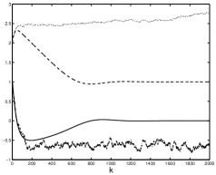
Figure 2: Evolution of $x_{k}$ (solid line) and $\hat{\theta}_{k}$ (dashed line) as functions of $k$ for the system (11) with NFC (22) ($\bar{\theta}=1$, $\hat{\theta}_{0}=2$, $x_{0}=1$, $a=1$, sampling period $T=0.01$ s). The curves in dash-dotted line and dotted line respectively show $x_{k}$ and $\hat{\theta}_{k}$ when $y_{k}$ is substituted for $x_{k}$ in (22).

Suppose now that the state is observed through $y_{0}=x_{0}$ and $y_{k}=x_{k}+\varepsilon_{k}$ for $k\geq 1$, where $(\varepsilon_{k})$ denotes a sequence of i.i.d. errors normal ${\mathcal{N}}(0,\sigma^{2})$ (setting $\sigma^{2}=S^{2}T$ one may suppose for instance that $\varepsilon_{k}$ is $S$ times the integral of a realization of the standard Brownian motion between 0 and $T$). We take $\sigma=x_{0}/2=0.5$, a rather extreme situation, to emphasize the influence of measurement errors. The evolutions of $x_{k}$ (dash-dotted line) and $\hat{\theta}_{k}$ (dotted line) when $y_{k}$ is substituted for $x_{k}$ in (22) are presented on Figure 2: the sequence of parameter estimates does not converge, the state fluctuates and is clearly not driven to zero.

7.3 Some consistency results

The difficulties encountered in Sections 7.1.1, 7.1.2 and 7.2 are general in regulation-type problems: in order to satisfy the control objective, the input should asymptotically vanish, which does not bring enough excitation for guaranteeing the consistent estimation of the model parameters. The control objective is thus in conflict with parameter estimation, and perturbations must be introduced. It is then of importance to know the minimal amount of perturbations required to ensure consistency of the estimator on which the control is based. Some results are presented below for the case of linear regression.

7.3.1 LS estimation

Consider a linear regression model with observations $y_{k}={\bf r}_{k}^{\top}\mbox{\boldmath$\bar{\theta}$}+\varepsilon_{k}$, and denote by ${\mathcal{F}}_{k}$ the $\sigma$-algebra generated by the errors $\varepsilon_{1},\ldots,\varepsilon_{k}$. They are supposed to form a martingale difference sequence ($\varepsilon_{k}$ is ${\mathcal{F}}_{k-1}$ measurable and ${\rm I}\!{\rm E}\{\varepsilon_{k}|{\mathcal{F}}_{k-1}\}=0$) and to be such that $\sup_{k}{\rm I}\!{\rm E}\{\varepsilon_{k}^{2}|{\mathcal{F}}_{k-1}\}<\infty$ (with i.i.d. errors with zero mean and finite variance as a special case). Let ${\bf M}_{N}=\sum_{k=1}^{N}{\bf r}_{k}{\bf r}_{k}^{\top}$, then ${\bf M}_{N}^{-1}\rightarrow 0$ for $N\rightarrow\infty$ is
$\bullet$ sufficient for $\mbox{\boldmath$\hat{\theta}$}_{LS}^{N}\stackrel{{\scriptstyle\rm a.s.}}{{\rightarrow}}\mbox{\boldmath$\bar{\theta}$}$ when the regressors ${\bf r}_{k}$ are non-random constants, see [97], [98];
$\bullet$ necessary and sufficient if, moreover, the errors are $\varepsilon_{k}$ i.i.d.,
$\bullet$ but ${\bf M}_{N}^{-1}\stackrel{{\scriptstyle\rm a.s.}}{{\rightarrow}}0$ is not sufficient for $\mbox{\boldmath$\hat{\theta}$}_{LS}^{N}\stackrel{{\scriptstyle\rm a.s.}}{{\rightarrow}}\mbox{\boldmath$\bar{\theta}$}$ if ${\bf r}_{k}$ is ${\mathcal{F}}_{k-1}$ measurable (see the first example of Section 7.1).

In the latter situation, a sufficient condition for $\mbox{\boldmath$\hat{\theta}$}_{LS}^{N}\stackrel{{\scriptstyle\rm a.s.}}{{\rightarrow}}\mbox{\boldmath$\bar{\theta}$}$ when $N\rightarrow\infty$ is that $\lambda_{\min}({\bf M}_{N})\stackrel{{\scriptstyle\rm a.s.}}{{\rightarrow}}\infty$ and $[\log\lambda_{\max}({\bf M}_{N})]^{1+\delta}=o[\lambda_{\min}({\bf M}_{N})]$ a.s. for some $\delta>0$, see [99]. In some sense, this is the best possible condition: it is only marginally violated in the first example of Section 7.1, where $[\log\lambda_{\max}({\bf M}_{N})]/\lambda_{\min}({\bf M}_{N})$ tends a.s. to a random constant. Note that this condition is much weaker than the persistence of excitation which requires that ${\bf M}_{N}$ grows at the same speed as $N$.

7.3.2 Bayesian imbedding

An even weaker condition is obtained for Bayesian estimation. Let $\pi$ be a prior probability measure for $\theta$ and denote by $P$ the probability measure induced by the errors $\varepsilon_{k}$, $k=1,\ldots,\infty$. Denote ${\mathcal{F}}^{\prime}_{k}$ the $\sigma$-algebra generated by the observations $y_{1},\ldots,y_{k}$ and suppose that ${\bf r}_{k}$ is ${\mathcal{F}}^{\prime}_{k-1}$-measurable. Suppose that the parameters are estimated by the posterior mean $\mbox{\boldmath$\hat{\theta}$}_{B}^{N}={\rm I}\!{\rm E}\{\mbox{\boldmath$\theta$}|{\mathcal{F}}^{\prime}_{N}\}$ and denote by ${\bf C}_{N}=\mbox{\rm Var}(\mbox{\boldmath$\theta$}|{\mathcal{F}}^{\prime}_{N})$ the posterior covariance matrix. Then, from martingale theory, $\mbox{\boldmath$\hat{\theta}$}_{B}^{N}$ and ${\bf C}_{N}$ both converge $(\pi\times P)$-a.s. when $N\rightarrow\infty$, see [174], and all what is required for the $(\pi\times P)$-a.s. consistency of the estimator is ${\bf C}_{N}\rightarrow 0$ $(\pi\times P)$-a.s. Now, for a linear regression model with i.i.d. normal errors $\varepsilon_{k}$ and a normal prior for $\theta$, Bayesian estimation coincides with LS estimation (when the prior for $\theta$ is suitably chosen), ${\bf C}_{N}$ is proportional to ${\bf M}_{N}^{-1}$ and therefore, ${\bf M}_{N}^{-1}\rightarrow 0$ $(\pi\times P)$-a.s. is sufficient for $\mbox{\boldmath$\hat{\theta}$}_{LS}^{N}=\mbox{\boldmath$\hat{\theta}$}_{B}^{N}\rightarrow\mbox{\boldmath$\bar{\theta}$}$ $(\pi\times P)$-a.s. The required condition is thus as weak as when the regressors ${\bf r}_{k}$ are non-random constants! Note, however, that the convergence is almost sure with respect to $\bar{\theta}$ having the prior $\pi$; that is, singular values of $\bar{\theta}$ may exist for which consistency does not hold.

This very powerful technique which analyses the properties of LS estimation via a Bayesian approach is called Bayesian imbedding, see [174], [93]. Although in its original formulation it requires the measurement errors to be normal, the normality assumption is relaxed in [68] to the condition that the density $\varphi$ of the errors is log-concave ($d^{2}\log\varphi(t)/dt^{2}<0$) and strictly positive with respect to the Lebesgue measure $\mu$, the prior measure $\pi$ being absolutely continuous with respect to $\mu$. More generally, the consistency of Bayesian estimators can be checked through the behavior of posterior covariance matrices, see [69]. Bayesian imbedding allows for easier proofs of consistency of the estimator, and permits to relax the conditions on the perturbations required to obtain consistency. This is illustrated below by revisiting the examples of Sections 7.1.1 and 7.1.2.

Consider again the self-tuning regulator of Section 7.1.1. When LS estimation is used with forced certainty equivalence control, it is required to perturb the system to obtain a globally convergent input. It can be shown [94] that the control objective $R_{n}$ grows at least as $\log n$, and randomly perturbed input sequences achieving this performance are proposed in [101]. Using Bayesian imbedding, global convergence can be obtained without the introduction of perturbations, see [93].

For the self-tuning optimizer of Section 7.1.2, Åström and Wittenmark [2] have suggested a control of the type ${\bf u}_{k+1}=\arg\max_{{\bf u}}f({\bf u},\mbox{\boldmath$\hat{\theta}$}^{k})+\alpha_{k}\ d({\bf u},\xi_{k})/k$, where $d({\bf u},\xi)={\bf r}^{\top}({\bf u}){\bf M}^{-1}(\xi){\bf r}({\bf u})$ is the function (17) used in $D$-optimal design, $\xi_{k}$ is the empirical measure of the inputs ${\bf u}_{1},\ldots,{\bf u}_{k}$ and $(\alpha_{k})$ is a sequence of positive scalars. Note that $d({\bf u},\xi_{k})/k={\bf r}^{\top}({\bf u}){\bf M}_{k}^{-1}{\bf r}({\bf u})$ with ${\bf M}_{k}=\sum_{i=1}^{k}{\bf r}({\bf u}_{i}){\bf r}^{\top}({\bf u}_{i})$. This strategy makes a compromise between optimization (maximization of $f({\bf u},\mbox{\boldmath$\hat{\theta}$}^{k})$, for $\alpha_{k}$ small) and estimation ($D$-optimal design, for $\alpha_{k}$ large). Using the results of Section 7.3.1, the following is proved in [135] for LS estimation. When the errors $\varepsilon_{k}$ form a martingale difference sequence with $\sup_{k}{\rm I}\!{\rm E}\{\varepsilon_{k}^{2}|{\mathcal{F}}_{k-1}\}<\infty$, if $(\alpha_{k}/k)\log\alpha_{k}$ is monotonically decreasing and $\alpha_{k}/(\log k)^{1+\delta}$ monotonically increases to infinity for some $\delta>0$, then $\mbox{\boldmath$\hat{\theta}$}_{LS}^{k}\stackrel{{\scriptstyle\rm a.s.}}{{\rightarrow}}\mbox{\boldmath$\bar{\theta}$}$, $(1/k)\sum_{i=1}^{k}f({\bf u}_{i},\mbox{\boldmath$\bar{\theta}$})\stackrel{{\scriptstyle\rm a.s.}}{{\rightarrow}}f({\bf u}^{*},\mbox{\boldmath$\bar{\theta}$})=\max_{\bf u}f({\bf u},\mbox{\boldmath$\bar{\theta}$})$ and $\xi_{k}\stackrel{{\scriptstyle\rm a.s.}}{{\rightarrow}}\delta_{{\bf u}^{*}}$ (weak convergence of probability measures) as $k\rightarrow\infty$. That is, the LS estimator is strongly consistent, and at the same time the design points ${\bf u}_{k}$ tend to concentrate at the optimal location ${\bf u}^{*}$. Using Bayesian imbedding, the same results are obtained when the conditions above on $\alpha_{k}$ are relaxed to $\alpha_{k}\rightarrow\infty$, $\alpha_{k}/k\rightarrow 0$, provided the errors $\varepsilon_{k}$ are i.i.d. ${\mathcal{N}}(0,\sigma^{2})$, see [141].

7.4 Finite horizon: dynamic programming and dual control

The presentation is for self-tuning optimization, but the problem is similar for other adaptive control situations. Suppose one wishes to maximize $\sum_{i=1}^{N}w_{i}f({\bf u}_{i},\mbox{\boldmath$\bar{\theta}$})$ for some sequence of positive weights $w_{i}$, with $\bar{\theta}$ unknown and estimated through observations $y_{i}=\eta(\mbox{\boldmath$\bar{\theta}$},{\bf u}_{i})+\varepsilon_{i}$. Let $\pi$ denote a prior probability measure for $\theta$ and define $U_{1}^{k}=({\bf u}_{1},\ldots,{\bf u}_{k})$, $Y_{1}^{k}=(y_{1},\ldots,y_{k})$ for all $k$. The problem to be solved can then be written as

$$\max_{{\bf u}_{1}}{\rm I}\!{\rm E}\{w_{1}f({\bf u}_{1},\mbox{\boldmath$\theta$})+\max_{{\bf u}_{2}}{\rm I}\!{\rm E}\{w_{2}f({\bf u}_{2},\mbox{\boldmath$\theta$})+\cdots$$

$$\hskip 28.45274pt\max_{{\bf u}_{N-1}}{\rm I}\!{\rm E}\{w_{N-1}f({\bf u}_{N-1},\mbox{\boldmath$\theta$})$$

$$\hskip 28.45274pt+\max_{{\bf u}_{N}}{\rm I}\!{\rm E}\{w_{N}f({\bf u}_{N},\mbox{\boldmath$\theta$})|U_{1}^{N-1},Y_{1}^{N-1}\}$$

$$\hskip 56.9055pt|U_{1}^{N-2},Y_{1}^{N-2}\}\cdots|{\bf u}_{1},y_{1}\}\}$$ (23)

and thus corresponds to a Stochastic Dynamic Programming (SDP) problem. It is, in general, extremely difficult to solve due to the presence of imbedded maximizations and expectations. The control ${\bf u}_{k}$ has a dual effect (see e.g. [7]): it affects both the value of $f({\bf u}_{k},\mbox{\boldmath$\theta$})$ and the future uncertainty on $\theta$ through the posterior measures $\pi(\mbox{\boldmath$\theta$}|U_{1}^{i},Y_{1}^{i})$, $i\geq k$. One of the main obstacles being the propagation of these measures, classical approaches are based on their approximation. Consider stage $k$, where $U_{1}^{k}$ and $Y_{1}^{k}$ are known. Then:
$\bullet$ Forced Certainty Equivalence control (FCE) replaces $\pi(\mbox{\boldmath$\theta$}|U_{1}^{i},Y_{1}^{i})$ for $i\geq k$ (a “future posterior” for $i>k$), by the delta measure $\delta_{\hat{\theta}^{k}}$, where $\mbox{\boldmath$\hat{\theta}$}^{k}$ is the current estimated value of $\theta$ (see the examples of Sections 7.1.1 and 7.1.2);
$\bullet$ Open-Loop-Feedback-Optimal control (OLFO) replaces $\pi(\mbox{\boldmath$\theta$}|U_{1}^{i},Y_{1}^{i})$, $i\geq k$, by the current posterior measure $\pi(\mbox{\boldmath$\theta$}|U_{1}^{k},Y_{1}^{k})$ (moreover, most often this posterior is approximated by a normal distribution ${\mathcal{N}}(\mbox{\boldmath$\hat{\theta}$}^{k},{\bf C}_{k})$).

The FCE and OLFO control strategies can be considered as passive since they ignore the influence of ${\bf u}_{k+1},{\bf u}_{k+2}\ldots$ on the future posteriors $\pi(\mbox{\boldmath$\theta$}|U_{1}^{i},Y_{1}^{i})$, see, e.g., [179]. On the other hand, they yield a drastic simplification of the problem, since the approximation of $\pi(\mbox{\boldmath$\theta$}|U_{1}^{i},Y_{1}^{i})$ for $i>k$ does not depend on the future observations $y_{k+1},y_{k+2}\ldots$ This, and the fact that few active alternatives exist, explains their frequent usage.

The active-control strategy suggested in [178] is based on a linearization around a nominal trajectory $\hat{\bf u}(i)$ and extended Kalman filtering. It does not seem to have been much employed, probably due to its rather high complexity. A modification of OLFO control is proposed in [137]. It takes a very simple form when the model response $\eta(\mbox{\boldmath$\theta$},{\bf u})$ is linear in $\theta$, that is, $\eta(\mbox{\boldmath$\theta$},{\bf u})={\bf r}^{\top}({\bf u})\mbox{\boldmath$\theta$}$, the errors are i.i.d. normal ${\mathcal{N}}(0,\sigma^{2})$ and the prior for $\theta$ is also normal. Then, at stage $k$, the posterior $\pi(\mbox{\boldmath$\theta$}|U_{1}^{i},Y_{1}^{i})$ is the normal ${\mathcal{N}}(\mbox{\boldmath$\hat{\theta}$}^{k}_{B},{\bf C}_{k})$ for $i=k$ and can be approximated by ${\mathcal{N}}(\mbox{\boldmath$\hat{\theta}$}^{k}_{B},{\bf C}_{i})$ for $i>k$, where $\mbox{\boldmath$\hat{\theta}$}^{k}_{B}$ and ${\bf C}_{k}$ are known (computed by classical recursive LS) and ${\bf C}_{i}$ follows a recursion similar to that of recursive LS,

$${\bf C}_{i+1}={\bf C}_{i}-\frac{{\bf C}_{i}{\bf r}({\bf u}_{i+1}){\bf r}^{\top}({\bf u}_{i+1}){\bf C}_{i}}{\sigma^{2}+{\bf r}^{\top}({\bf u}_{i+1}){\bf C}_{i}{\bf r}({\bf u}_{i+1})}\,,\ \ i\geq k\,.$$

Note that ${\bf C}_{i}$ depends of ${\bf u}_{k+1},{\bf u}_{k+2}\ldots,{\bf u}_{i}$ (which makes the strategy active), but not on $y_{k+1},y_{k+2}\ldots$ (which makes it implementable). This method has been successfully applied to the adaptive control of model with a FIR, ARX, or state-space structure, see, e.g., [91], [92]. It requires, however, that the objective function $f({\bf u},\mbox{\boldmath$\theta$})$ in (23) be non linear in $\theta$ to express the dependence in the covariance matrices ${\bf C}_{i}$. Indeed, suppose that in the self-tuning optimization problem the function to be maximized is the model response itself, that is, $f({\bf u},\mbox{\boldmath$\theta$})={\bf r}^{\top}({\bf u})\mbox{\boldmath$\theta$}$. Then, ${\rm I}\!{\rm E}\{f({\bf u},\mbox{\boldmath$\theta$})|U_{1}^{i},Y_{1}^{i}\}={\bf r}^{\top}({\bf u})\mbox{\boldmath$\hat{\theta}$}^{i}_{B}$ and using the approximation ${\mathcal{N}}(\mbox{\boldmath$\hat{\theta}$}^{k}_{B},{\bf C}_{i})$ for the future posteriors $\pi(\mbox{\boldmath$\theta$}|U_{1}^{i},Y_{1}^{i})$, $i>k$, one gets classical FCE control based on the Bayesian estimator $\mbox{\boldmath$\hat{\theta}$}^{k}_{B}$. On the other hand, it is possible in that case to take benefit of the linearity of the function and obtain an approximation of ${\rm I}\!{\rm E}\{\max_{\bf u}{\bf r}^{\top}({\bf u})\mbox{\boldmath$\hat{\theta}$}^{N-1}_{B}|U_{1}^{N-2},Y_{1}^{N-2}\}$ for small $\sigma^{2}$, which can then be back-propagated; see [141] where a control strategy is given that is within ${\mathcal{O}}(\sigma^{4})$ of the optimal (unknown) strategy ${\bf u}_{k}^{*}$ for the SDP problem (23).

8 Sequential DOE

Consider a nonlinear regression model for which the optimal design problem consists in minimizing $\Psi_{\bar{\theta}}(U_{1}^{N})=\Phi[{\bf M}_{F}(U_{1}^{N},\mbox{\boldmath$\bar{\theta}$})]$ for some criterion $\Phi$, with $\bar{\theta}$ unknown. In order to design an experiment adapted to $\bar{\theta}$, a natural approach consists in working sequentially. In full-sequential design, one support point ${\bf u}_{k}$ is introduced after each observation: $\mbox{\boldmath$\hat{\theta}$}^{k-1}$ is estimated from the data $(Y_{1}^{k-1},U_{1}^{k-1})$ and next ${\bf u}_{k}$ minimizes $\Phi[{\bf M}_{F}(\{U_{1}^{k-1},{\bf u}_{k}\},\mbox{\boldmath$\hat{\theta}$}^{k-1})]$ (for $D$-optimal design, this is equivalent to choosing ${\bf u}_{k}$ that maximizes $d_{\hat{\theta}^{k-1}}({\bf u}_{k},\xi_{k-1})$ with $d_{\theta}({\bf u},\xi)$ the function (17) and $\xi_{k-1}$ the empirical measure for the design points in $U_{1}^{k-1}$). Note that it may be considered as a FCE control strategy, where the input (design point) at step $k$ is based on the current estimated value $\mbox{\boldmath$\hat{\theta}$}^{k-1}$. For a finite horizon $N$ (the number of observations), the problem is similar to that of Section 7.4 (self-tuning optimizer), with the design objective $\Phi[{\bf M}_{F}(U_{1}^{N},\mbox{\boldmath$\theta$})]$ substituted for $\sum_{i=1}^{N}w_{i}f({\bf u}_{i},\mbox{\boldmath$\theta$})$. Although the objective does not take an additive form, the problem is still of the SDP type, and active-control strategies can thus be constructed to approximate the optimal solution. However, they seem to only provide marginal improvements over traditional passive strategies like FCE control, see e.g. [51].

Although a sequentially designed experiment for the minimization of $\Phi[{\bf M}_{F}(U_{1}^{N},\mbox{\boldmath$\theta$})]$ aims at estimating $\theta$ with maximum possible precision, it is difficult to assess that $\mbox{\boldmath$\hat{\theta}$}^{N}\stackrel{{\scriptstyle\rm a.s.}}{{\rightarrow}}\mbox{\boldmath$\bar{\theta}$}$ as $N\rightarrow\infty$ (and thus $\xi_{N}\stackrel{{\scriptstyle\rm a.s.}}{{\rightarrow}}\xi^{*}(\mbox{\boldmath$\bar{\theta}$})$, with $\xi^{*}(\mbox{\boldmath$\bar{\theta}$})$ the optimal design for $\bar{\theta}$) when full-sequential design is used; see [191] for a simple example (with a positive answer) for LS estimation. When full-sequential design is based on Bayesian estimation (posterior mean), strong consistency can be proved if the optimal design $\xi^{*}(\mbox{\boldmath$\theta$})$ satisfies an identifiability condition for any $\theta$, see [70] (this is related to Bayesian imbedding considered in Section 7.3.2). The asymptotic analysis of multi-stage sequential design is considered in [28] and the construction of asymptotically optimal sequential design strategies in [172], where it is shown that using two stages is enough. Practical experience tends to confirm the good performance of two-stage procedures, see, e.g., [8].

9 Concluding remarks and perspectives in DOE

Correlated errors. Few results exist on DOE in the presence of correlated observations and one can refer e.g. to [127], [117], [45] and the monograph [116] for recent developments. See also Section 3.2.2. The situation is different in the adaptive control community where correlated errors are classical, see Section 7.3.1 (for instance, the paper [123] gives results on strong laws of large numbers for correlated sequences of random variables under rather common assumptions in signal or control applications), which calls for appropriate developments in DOE. Notice that when the correlation of the error process decays at hyperbolic rate (long-range dependence), the asymptotic theory of parameter estimation in regression models (Section 4) must itself be revisited, see, e.g., [73].

Nonlinear models. The presentation in Sections 6 and 7 has concerned models with a linear dynamic (e.g. with a Box and Jenkins structure), but models that corresponds to nonlinear differential or recurrence equations raise no special difficulty for the construction of the Fisher information matrix (Section 6), which can always be obtained through simulations. The main issue concerns linearity with respect to the model parameters $\theta$. In particular, few results exist concerning the extension of the results of Section 7.3 to models with a nonlinear parametrization (see [95] for LS estimation and [71] for results on Bayesian imbedding when $\theta$ has a discrete prior).

DOE without persistence of excitation. In the context of self-tuning regulation, we mentioned in Section 7.3.2 that random perturbations may be added to certainty equivalence control based on LS estimation to guarantee the strong consistency of parameter estimates and the asymptotically optimal growth of the control objective, see [101]. This is an example of a situation where “non-stationary experiments” could be designed in order to replace random perturbations by inputs with suitable spectrum and asymptotically vanishing amplitude. In the same vein, the modified OLFO control proposed in [137] and the small-noise approximation of [141] (designed for self-tuning optimization, but extendable to self-tuning regulation) make a good compromise between exploration and exploitation when the horizon is finite (see Section 7.4). An asymptotic analysis for the horizon tending to infinity could permit to design simpler non-stationary strategies.

Nonparametric models, active learning and control. Strategies are called active in opposition to passive ones that collect data “as they come”. DOE is thus intrinsically active, and its use in learning leads to methods that try to select training samples instead of taking them randomly. Although its usefulness is now well perceived in the statistical learning community, it is still at an early stage of development due to the complexity of DOE for nonparametric models. More generally, active strategies are valuable each time actions or decisions have a dual effect and a compromise should be made between exploration and exploitation: exploration may be done at random, but better performance is achieved when it is carefully planned. For instance, active strategies connected with Markov decision theory could yield improvements in reinforcement learning, see e.g. the survey [80].

Linking nonparametric estimation with control forms a quite challenging area, where the issues raised by the estimation of the function that defines the dynamics of the system come in addition to those, more classical, of adaptive control with parametric models, see, e.g., [134], [133] for emerging developments.

Algorithms for optimal DOE. The importance of constructing criteria for DOE in relation with the intended objective has been underlined in Section 6.2 where criteria of the minimax type have been introduced from robust-control considerations. (Minimax-optimal design is also an efficient method to face the dependence of local optimal design in the unknown value of the model parameters, see Section 5.3.5.) Although the minimax problem can often be formulated as a convex one, sometimes with a finite number of constraints, the development of specific algorithms would be much profitable to the diffusion of the methodology, in the same way as the classical design algorithms of Sections 5.2 and 5.3.3 have contributed to the diffusion of optimal DOE outside the statistical community where it originated.

Another view on global optimization. Let $f({\bf u})$ be a function to be maximized with respect to ${\bf u}$ in some given set ${\mathcal{U}}$; it is not assumed to be concave, nor is the set ${\mathcal{U}}$ assumed to be convex, so that local maxima may exist. The function can be evaluated at any given input ${\bf u}_{i}\in{\mathcal{U}}$, which gives an “observation” $y({\bf u}_{i})=f({\bf u}_{i})$. In engineering applications where the evaluation of $f$ corresponds to the execution of a large simulation code, expensive in terms of computing time, it is of paramount importance to use an optimization method parsimonious in terms of number of function evaluations. This enters into the framework of computer experiments, where Kriging is now a rather well-established tool for modelling, see Section 3.1. Using a Bayesian point of view, the value $f({\bf u})$ after the collection of the data ${\mathcal{D}}_{k}=\{[{\bf u}_{1},y({\bf u}_{1})],\ldots,[{\bf u}_{k},y({\bf u}_{k})]\}$ can be considered as distributed with the density $\varphi(y|{\mathcal{D}}_{k},{\bf u})$ of the normal distribution ${\mathcal{N}}(\hat{y}_{{\mathcal{D}}_{k}}({\bf u}),\rho^{2}_{{\mathcal{D}}_{k}}({\bf u}))$, where $\hat{y}_{{\mathcal{D}}}({\bf u})$ and $\rho^{2}_{{\mathcal{D}}}({\bf u})$ are respectively given by (3) and (4). An optimization algorithm that uses this information should then make a compromise between exploration (trying to reduce the MSE $\rho^{2}_{{\mathcal{D}}}({\bf u})$ by placing observations at values of ${\bf u}$ where $\rho^{2}_{{\mathcal{D}}}({\bf u})$ is large) and exploitation (trying to maximize the expected response $\hat{y}_{{\mathcal{D}}}({\bf u})$). A rather intuitive method is to choose ${\bf u}_{k+1}$ that maximizes $\hat{y}_{{\mathcal{D}}_{k}}({\bf u})+\alpha\rho_{{\mathcal{D}}_{k}}({\bf u})$ for some positive constant $\alpha$, see [35]. In theory, Stochastic Dynamic Programming could be used to find the optimal strategy (or algorithm) to maximize $f({\bf u})$: when the number $N$ of evaluations is given in advance, the problem takes the same form as in (23) with $w_{i}=0$ for $i=1,\ldots,N-1$. However, in practise this SDP problem is much too difficult to solve, and approximations must be used to define suboptimal searching rules. For instance, one may use a one-step-ahead approach and choose the input ${\bf u}_{k+1}$ that maximizes the expected improvement $EI({\bf u})=\int^{\infty}_{y_{k}^{\max}}[y-y_{k}^{\max}]\,\varphi(y|{\mathcal{D}}_{k},{\bf u})\,dy$, with $y_{k}^{\max}=\max\{y({\bf u}_{1}),\ldots,y({\bf u}_{k})\}$, the maximum value of $f$ observed so far, see [110], [109], [161]. The function $f$ is then evaluated at ${\bf u}_{k+1}$, the Kriging model is updated (although not necessarily at each iteration), and similar steps are repeated. Each iteration of the resulting algorithm requires one evaluation of $f$ and the solution of another global optimization problem, for which any ad-hoc global search algorithm can be used (the optimization concerns the function $EI$, which is easier to evaluate than $f$). For instance, it is suggested in [11] to update a Delaunay triangulation of the set ${\mathcal{U}}$ based on the vertices ${\bf u}_{i}$, $i=1,\ldots,k$, and to perform the global search for the maximization of $EI({\bf u})$ by initializing local searches at the centers of the Delaunay cells. Note that the algorithm tends asymptotically to observe everywhere in ${\mathcal{U}}$, since the expected improvement $EI({\bf u})$ is always strictly positive at any value ${\bf u}$ where no observation has been taken yet. However, a credible stopping rule is given by the criterion itself: it is reasonable to stop when the expected improvement becomes small enough. One can refer to [161], [79] for detailed implementations, including problems with constraints also defined by simulation codes. Derivative information on $f$ can be included in the Kriging model, as indicated in Section 3.1, and thus used by the optimization algorithm, see [102]. It seems that suboptimal searching rules looking further than one-step-ahead have never been used, which forms a rather challenging objective for active control. Also, the one-step-ahead method above is completely passive with respect to the estimation of the parameters of the Kriging model, and active strategies (even one-step-ahead) are still to be designed, see Section 3.2.2. Note finally that the definition of the expected improvement $EI$ is not adapted to the presence of errors in the evaluation of $f$, so that further developments are required for situations where one optimizes the observed response of a real physical process.

NFC, FCE, estimating functions and DOE. Consider again the example of NFC in Section 7.2, in the case where the state $x_{k}$ is observed though $y_{k}=x_{k}+\varepsilon_{k}$ and $y_{k}$ is substituted for $x_{k}$ in (22). As shown in Figure 2, the NFC estimator $\hat{\theta}_{k}$ is then not consistent. On the other hand, in the same situation more classical estimation techniques have satisfactory behaviors (hence, in terms of DOE, NFC brings enough information to estimate the unknown $\bar{\theta}$). Consider for instance the LS estimator of $\bar{\theta}$ in (11), obtained from $y_{1},\ldots,y_{k}$. Since $x_{k}$ is nonlinear in $\theta$, recursive LS cannot be used directly, but the estimation becomes almost recursive using a stochastic-Newton algorithm, see, e.g., [188], p. 208. Figure 3 (top) shows that the corresponding estimator $\hat{\theta}^{k}$ converges quickly to the true value $\bar{\theta}=1$. The evolution of the estimator (13) obtained from an estimating function is presented on the same figure (bottom). Its convergence is slower than that of $\hat{\theta}^{k}$, due in particular to the presence of the term $y_{k}/(kT)$ in the numerator of (13), but its construction is much simpler. An important consequence is that the analysis of its asymptotic behavior in an adaptive-control framework is easier than for LS estimation: $\tilde{\theta}^{k}$ is a consistent estimator of $\bar{\theta}$ when $(1/k)\sum_{i=1}^{k-1}x_{i}$ is bounded away from $-1$ (which is the case since the control drives this quantity to zero). Simulations confirm that when applying the FCE controller $u_{k}=-(a+\tilde{\theta}^{k})\hat{x}_{k}(\tilde{\theta}^{k})-\tilde{\theta}^{k}$ to (11), with $\hat{x}_{k}(\tilde{\theta}^{k})$ obtained by substituting $\tilde{\theta}^{k}$ for $\bar{\theta}$ in (11), $\tilde{\theta}^{k}$ converges to $\bar{\theta}$ and the state $x_{k}$ is correctly driven to zero. Simulations show, however, that the dynamic of the state is slower than for NFC; it is thus tempting to combine both strategies. For instance, one could use FCE control based on $\tilde{\theta}^{k}$ when the standard deviation of $\tilde{\theta}^{k}$ is smaller than some prescribed value, and use NFC otherwise. The simulation results obtained with such a switching strategy are encouraging and indicate that the combination of different estimation methods may improve the performance of the controller. At the same time, this raises more issues than it brings answers. Some are listed below.

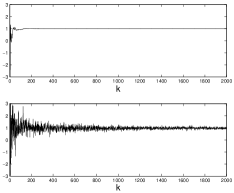
Figure 3: Top: evolution of the LS estimator $\hat{\theta}^{k}$; bottom: evolution of $\tilde{\theta}^{k}$ given by (13).

Combining NFC, which relies on Lyapunov stability, with simple predictors, e.g. based on FCE, while preserving stability, forms an interesting challenge for which results on input-to-state stabilizing control could be used (see, e.g., Chapters 5 and 6 of [88] for continuous-time and [121] for discrete-time control). In classical FCE control the consistency of the estimator is a major issue. Using suitable estimating functions could then lead to fruitful developments, due the flexibility of the method and the simplicity of the associated estimators. Suitably designed perturbations could be introduced for helping the estimation, possibly following developments similar to those that lead to the active-control strategies of Sections 7.3.2 and 7.4. At the same time, the perturbed control should not endanger the stability of the system. Designing input sequences (possibly vanishing with time) that bring maximum information for estimation subject to a stability constraint forms an unusual and challenging DOE problem. Finally, as a first step towards the design of robust-and-adaptive controllers mentioned at the end of Section 6.2, one may replace a traditional FCE controller by one that gives the best performance for the worst model in the current uncertainty set (roughly speaking, for the self-tuning problem considered in Section 7.4 this amounts to replacing expectations in (23) by minimizations with respect to $\theta$ in the current uncertainty set). The determination of active-control strategies for such minimax (dynamical games) problems seems to be a promising direction for developments in adaptive control.

This work was partially supported by the IST Programme of the European Community, under the PASCAL Network of Excellence, IST-2002-506778. This publication only reflects the authors’s view. The paper is partly based on a three-hours mini-course given at the 24th Benelux Meeting at Houffalize, Belgium, on March 22-24, 2005. It has benefited from several interesting and motivating discussions during that meeting, and the organizers of the event are gratefully acknowledged for their invitation. Many ideas and references result from many years of collaboration with Éric Walter (CNRS/SUPELEC/Université Paris XI, France), Andrej Pázman (Comenius University, Bratislava, Slovakia), Henry P. Wynn (LSE, London, UK) and Anatoly A. Zhigljavsky (Cardiff University, UK). Sections 7.3.2 and 9 have benefited from several discussions with Éric Thierry and Tarek Hamel at I3S. The encouraging comments and suggestions of several referees were also much helpful.

References

- [1] K.J. Åström and B. Wittenmark. On self-tuning regulators. Automatica, 9:195–199, 1973.
- [2] K.J. Åström and B. Wittenmark. Adaptive Control. Addison Wesley, 1989.
- [3] A.C. Atkinson and D.R. Cox. Planning experiments for discriminating between models (with discussion). Journal of Royal Statistical Society, B36:321–348, 1974.
- [4] A.C. Atkinson and A.N. Donev. Optimum Experimental Design. Oxford University Press, 1992.
- [5] A.C. Atkinson and V.V. Fedorov. The design of experiments for discriminating between two rival models. Biometrika, 62(1):57–70, 1975.
- [6] A.C. Atkinson and V.V. Fedorov. Optimal design: experiments for discriminating between several models. Biometrika, 62(2):289–303, 1975.
- [7] Y. Bar-Shalom and E. Tse. Dual effect, certainty equivalence, and separation in stochastic control. IEEE Transactions on Automatic Control, 19(5):494–500, 1974.
- [8] M. Barenthin, H. Jansson, and H. Hjalmarsson. Applications of mixed and input design in identification. In Proc. 16th IFAC World Congress on Automatic Control, Prague, 2005. CD-ROM – Paper 03882.
- [9] H.A. Barker and K.R. Godfrey. System identification with multi-level periodic perturbation signals. Control Engineering Practice, 7:717–726, 1999.
- [10] P.L. Bartlett. Prediction algorithms: complexity, concentration and convexity. In Prep. 13th IFAC Symposium on System Identification, Rotterdam, pages 1507–1517, August 2003.
- [11] R. Bates and L. Pronzato. Emulator-based global optimisation using lattices and Delaunay tesselation. In P. Prado and R. Bolado, editors, Proc. 3rd Int. Symp. on Sensitivity Analysis of Model Output, pages 189–192, Madrid, June 2001.
- [12] S. Biedermann and H. Dette. Minimax optimal designs for nonparametric regression — a further optimality property of the uniform distribution. In P. Hackl A.C. Atkinson and W.G. Müller, editors, mODa’6 – Advances in Model–Oriented Design and Analysis, Proceedings of the 76th Int. Workshop, Puchberg/Schneberg (Austria), pages 13–20, Heidelberg, June 2001. Physica Verlag.
- [13] D. Böhning. Likelihood inference for mixtures: geometrical and other constructions of monotone step-length algorithms. Biometrika, 76(2):375–383, 1989.
- [14] X. Bombois, B.D.O. Anderson, and M. Gevers. Quantification of frequency domain error bounds with guaranteed confidence level in prediction error identification. System & Control Letters, 54:471–482, 2005.
- [15] X. Bombois, G. Scorletti, M. Gevers, R. Hildebrand, and P. Van den Hof. Cheapest open-loop identification for control. In Proc. 43rd Conf. on Decision and Control, pages 382–387, The Bahamas, December 2004.
- [16] X. Bombois, G. Scorletti, M. Gevers, P. Van den Hof, and R. Hildebrand. Least costly identification experiment for control. Automatica, 42(10):1651–1662, 2006.
- [17] G.E.P. Box and W.J. Hill. Discrimination among mechanistic models. Technometrics, 9(1):57–71, 1967.
- [18] G.E.P. Box and K.B. Wilson. On the experimental attainment of optimum conditions (with discussion). Journal of Royal Statistical Society, B13(1):1–45, 1951.
- [19] M.J. Box. Bias in nonlinear estimation. Journal of Royal Statistical Society, B33:171–201, 1971.
- [20] S. Boyd, L. El Ghaoui, E. Feron, and V. Balakrishnan. Linear Matrix Inequalities in System and Control Theory. SIAM, Philadelphia, 1994.
- [21] S. Boyd and L. Vandenberghe. Convex Optimization. Cambridge University Press, Cambridge, 2004.
- [22] A.S. Bozin and M.B. Zarrop. Self tuning optimizer — convergence and robustness properties. In Proc. 1st European Control Conf., pages 672–677, Grenoble, July 1991.
- [23] L. Breiman. Bagging predictors. Machine Learning, 24(2):123–140, 1996.
- [24] P.E. Caines. Linear Stochastic Systems. Wiley, New York, 1988.
- [25] M.C. Campi and E. Weyer. Guaranteed non-asymptotic confidence regions in system identification. Automatica, 41(10):1751–1764, 2005.
- [26] K. Chaloner and K. Larntz. Optimal Bayesian design applied to logistic regression experiments. Journal of Statistical Planning and Inference, 21:191–208, 1989.
- [27] K. Chaloner and I. Verdinelli. Bayesian experimental design: a review. Statistical Science, 10(3):273–304, 1995.
- [28] P. Chaudhuri and P.A. Mykland. Nonlinear experiments: optimal design and inference based likelihood. Journal of the American Statistical Association, 88(422):538–546, 1993.
- [29] C.S. Chen. Optimality of some weighing and fractional factorial designs. Annals of Statistics, 8:436–446, 1980.
- [30] M.-Y Cheng, P. Hall, and D.M. Titterington. Optimal design for curve estimation by local linear smoothing. Bernoulli, 4(1):3–14, 1998.
- [31] H. Chernoff. Locally optimal designs for estimating parameters. Annals of Math. Stat., 24:586–602, 1953.
- [32] J.-Y. Choi, M. Krstić, K.B. Ariyur, and J.S. Lee. Extremum seeking control for discrete-time systems. IEEE Transactions on Automatic Control, 47(2):318–323, 2002.
- [33] D.A. Cohn. Neural network exploration using optimal experiment design. In J. Cowan, G. Tesauro, and J. Alspector, editors, Advances in Neural Information Processing Systems 6. Morgan Kaufmann, 1994.
- [34] D.A. Cohn, Z. Ghahramani, and M.I. Jordan. Active learning with statistical models. Journal of Artificial Intelligence Research, 4:129–145, 1996.
- [35] D.D. Cox and S. John. A statistical method for global optimization. In Proc. IEEE Int. Conf. on Systems Man and Cybernetics, volume 2, pages 1241–1246, Chicago, IL, October 1992.
- [36] D.R. Cox and D.V. Hinkley. Theoretical Statistics. Chapman & Hall, London, 1974.
- [37] F. Cucker and S. Smale. On the mathematical foundations of learning. Bulletin of the AMS, 39(1):1–49, 2001.
- [38] C. Currin, T.J. Mitchell, M.D. Morris, and D. Ylvisaker. Bayesian prediction of deterministic functions, with applications to the design and analysis of computer experiments. Journal of the American Statistical Association, 86:953–963, 1991.
- [39] D.Z. D’Argenio. Optimal sampling times for pharmacokinetic experiments. Journal of Pharmacokinetics and Biopharmaceutics, 9(6):739–756, 1981.
- [40] D. den Hertog. Interior Point Approach to Linear, Quadratic and Convex Programming. Kluwer, Dordrecht, 1994.
- [41] J.J. Faraway. Sequential design for the nonparametric regression of curves and surfaces. Computing Science and Statistics, 22:104–110, 1990.
- [42] V.V. Fedorov. Theory of Optimal Experiments. Academic Press, New York, 1972.
- [43] V.V. Fedorov. Convex design theory. Math. Operationsforsch. Statist., Ser. Statistics, 11(3):403–413, 1980.
- [44] V.V. Fedorov and P. Hackl. Model-Oriented Design of Experiments. Springer, Berlin, 1997.
- [45] V.V. Fedorov and W.G. Müller. Optimum design for correlated processes via eigenfunction expansions. Department of Statistics and Mathematics, Wirtschaftsuniversität Wien, Report 6, June 2004.
- [46] R.A. Fisher. Statistical Methods for Research Workers. Oliver & Boyd, Edimbourgh, 1925.
- [47] M. Fliess and H. Sira-Ramiírez. An algebraic framework for linear identification. ESAIM: Control, Optimization and Calculus of Variations, (9):151–168, 2003.
- [48] A. Forsgren, P.E. Gill, and M.H. Wright. Interior methods for nonlinear optimization. SIAM Review, 44(4):525–597, 2002.
- [49] U. Forssell and L. Ljung. Closed-loop identification revisited. Automatica, 35:1215–1241, 1999.
- [50] U. Forssell and L. Ljung. Some results on optimum experiment design. Automatica, 36:749–756, 2000.
- [51] R. Gautier and L. Pronzato. Adaptive control for sequential design. Discussiones Mathematicae, Probability & Statistics, 20(1):97–114, 2000.
- [52] S. Gazut, J.-M. Martinez, and S. Issanchou. Plans d’expériences itératifs pour la construction de modèles non linéaires. In CD – 38èmes Journées de Statistique de la SFdS, Clamart, France, 2006.
- [53] M. Gevers. Identification for control. From the early achievements to the revival of experimental design. European Journal of Control, 11(45):335–352, 2005.
- [54] M. Gevers, X. Bombois, B. Codrons, G. Scorletti, and B.D.O. Anderson. Model validation for control and controller validation in a prediction error identification framework — Part I: theory. Automatica, 39:403–415, 2003.
- [55] M. Gevers, X. Bombois, B. Codrons, G. Scorletti, and B.D.O. Anderson. Model validation for control and controller validation in a prediction error identification framework — Part II: illustrations. Automatica, 39:417–427, 2003.
- [56] M. Gevers and L. Ljung. Benefits of feedback in experiment design. In Prep. 7th IFAC/IFORS Symp. on Identification and System Parameter Estimation, pages 909–914, York, 1985.
- [57] M. Gevers and L. Ljung. Optimal experiment design with respect to the intended model application. Automatica, 22:543–554, 1986.
- [58] G.C. Goodwin and R.L. Payne. Dynamic System Identification: Experiment Design and Data Analysis. Academic Press, New York, 1977.
- [59] G.C. Goodwin and M.E. Salgado. A stochastic imbedding approach for quantifying uncertainty in the estimation of restricted complexity models. International Journal of Adaptive Control and Signal Processing, 3:333–356, 1989.
- [60] L. Guo. Further results on least-squares based adaptive minimum variance control. SIAM J. Control and Optimization, 32(1):187–212, 1994.
- [61] R. Harman and L. Pronzato. Improvements on removing non-optimal support points in D-optimum design algorithms. Statistics & Probability Letters, 77:90–94, 2007.
- [62] T. Hastie, R. Tibshirani, and J. Friedman. The Elements of Statistical Learning. Data Mining, Inference and Prediction. Springer, Heidelberg, 2001.
- [63] C.C. Heyde. Quasi-likelihood and its Application. A General Approach to Optimal Parameter Estimation. Springer, New York, 1997.
- [64] R. Hildebrand and M. Gevers. Identification for control: optimal input design with respect to a worst-case -gap cost function. SIAM Journal on Control and Optimization, 42(5):1586–1608, 2003.
- [65] P.D.H. Hill. A review of experimental design procedures for regression model discrimination. Technometrics, 20:15–21, 1978.
- [66] H. Hjalmarsson. From experiment design to closed-loop control. Automatica, 41:393–438, 2005.
- [67] H. Hjalmarsson, M. Gevers, and F. De Bruyne. For model-based control design, closed-loop identification gives better performance. Automatica, 32(12):1659–1673, 1996.
- [68] I. Hu. Strong consistency of Bayes estimates in stochastic regression models. Journal of Multivariate Analysis, 57:215–227, 1996.
- [69] I. Hu. Strong consistency in stochastic regression models via posterior covariance matrices. Biometrika, 84(3):744–749, 1997.
- [70] I. Hu. On sequential designs in nonlinear problems. Biometrika, 85(2):496–503, 1998.
- [71] I. Hu. Strong consistency of Bayes estimates in nonlinear stochastic regression models. Journal of Statistical Planning and Inference, 67:155–163, 1998.
- [72] P.J. Huber. Robust Statistics. John Wiley, New York, 1981.
- [73] A.V. Ivanov and N.N. Leonenko. Asymptotic theory of nonlinear regression with long-range dependence. Mathematical Methods of Statistics, 13(2):153–178, 2004.
- [74] H. Jansson and H. Hjalmarsson. Mixed and input design for identification. In Proc. 43rd Conf. on Decision and Control, pages 388–393, The Bahamas, December 2004.
- [75] H. Jansson and H. Hjalmarsson. Input design via LMIs admitting frequency-wise model specifications in confidence regions. IEEE Transactions on Automatic Control, 50(10):1534–1549, 2005.
- [76] H. Jansson and H. Hjalmarsson. Optimal experiment design in closed loop. In Proc. 16th IFAC World Congress on Automatic Control, Prague, 2005. CD-ROM – Paper 04528.
- [77] R.I. Jennrich. Asymptotic properties of nonlinear least squares estimation. Annals of Math. Stat., 40:633–643, 1969.
- [78] M.E. Johnson, L.M. Moore, and D. Ylvisaker. Minimax and maximin distance designs. Journal of Statistical Planning and Inference, 26:131–148, 1990.
- [79] D. Jones, M. Schonlau, and W.J. Welch. Efficient global optimization of expensive black-box functions. Journal of Global Optimization, 13:455–492, 1998.
- [80] L.P. Kaelbling, M.L. Littman, and A.W. Moore. Reinforcement learning: a survey. Journal of Artificial Intelligence Research, 4:237–285, 1996.
- [81] T. Kanamori. Statistical asymptotic theory of active learning. Annals Inst. Statist. Math., 54(3):459–475, 2002.
- [82] F. Kerestecioğlu. Change Detection and Input Design in Dynamical Systems. Research Studies Press, Taunton, UK, 1993.
- [83] J. Kiefer and J. Wolfowitz. Stochastic estimation of the maximum of a regression function. Annals of Math. Stat., 23:462–466, 1952.
- [84] J. Kiefer and J. Wolfowitz. Optimum designs in regression problems. Annals of Math. Stat., 30:271–294, 1959.
- [85] J. Kiefer and J. Wolfowitz. The equivalence of two extremum problems. Canadian Journal of Mathematics, 12:363–366, 1960.
- [86] D.G. Krige. A statistical approach to some mine valuation and allied problems on the Witwatersrand. Master Thesis, University of Witwatersrand, 1951.
- [87] M. Krstić. Performance improvement and limitations in extrremum seeking control. System & Control Letters, 39:313–326, 2000.
- [88] M. Krstić, I. Kanellakopoulos, and P. Kokotović. Nonlinear and Adaptive Control Design. Wiley, New York, 1995.
- [89] M. Krstić and H.-H. Wang. Stability of extremum seeking feedback for general nonlinear dynamic systems. Automatica, 36:595–601, 2000.
- [90] C.S. Kubrusly and H. Malebranche. Sensors and controllers location in distributed systems—A survey. Automatica, 21(2):117–128, 1985.
- [91] C. Kulcsár, L. Pronzato, and E. Walter. Dual control of linearly parameterised models via prediction of posterior densities. European J. of Control, 2(1):135–143, 1996.
- [92] C. Kulcsár, L. Pronzato, and E. Walter. Experimental design for the control of linear state-space systems. In Proc. 13th IFAC World Congress, volume C, pages 175–180, San Francisco, June 1996.
- [93] P.R. Kumar. Convergence of adaptive control schemes using least-squares parameter estimates. IEEE Transactions on Automatic Control, 35(4):416–424, 1990.
- [94] T.L. Lai. Asymptotically efficient adaptive control in stochastic regression models. Advances in Applied Math., 7(23):23–45, 1986.
- [95] T.L. Lai. Asymptotic properties of nonlinear least squares estimates in stochastic regression models. Annals of Statistics, 22(4):1917–1930, 1994.
- [96] T.L. Lai and H. Robbins. Consistency and asymptotic efficiency of slope estimates in stochastic approximation schemes. Z. Wahrsch. verw. Gebiete, 56:329–360, 1981.
- [97] T.L. Lai, H. Robbins, and C.Z. Wei. Strong consistency of least squares estimates in multiple regression. Proc. Nat. Acad. Sci. USA, 75(7):3034–3036, 1978.
- [98] T.L. Lai, H. Robbins, and C.Z. Wei. Strong consistency of least squares estimates in multiple regression II. Journal of Multivariate Analysis, 9:343–361, 1979.
- [99] T.L. Lai and C.Z. Wei. Least squares estimates in stochastic regression models with applications to identification and control of dynamic systems. Annals of Statistics, 10(1):154–166, 1982.
- [100] T.L. Lai and C.Z. Wei. On the concept of excitation in least squares identification and adaptive control. Stochastics, 16:227–254, 1986.
- [101] T.L. Lai and C.Z. Wei. Asymptotically efficient self-tuning regulators. SIAM J. Control and Optimization, 25(2):466–481, 1987.
- [102] S. Leary, A. Bhaskar, and A.J. Keane. A derivative based surrogate model for approximating and optimizing the output of an expensive computer simulation. Journal of Global Optimization, 30:39–58, 2004.
- [103] K.-Y. Liang and S.L. Zeger. Inference based on estimating functions in the presence of nuisance parameters. Statistical Science, 10(2):158–173, 1995.
- [104] L. Ljung. System Identification, Theory for the User. Prentice-Hall, Englewood Cliffs, 1987.
- [105] K.V. Mardia. Maximum likelihood estimation for spatial models. In D.A. Griffith, editor, Spatial Statistics: Past, Present and Future, pages 203–253. Michigan Document Services, Ann Arbor, Michigan, 1990.
- [106] K.V. Mardia, J.T. Kent, C.R. Goodall, and J.A. Little. Kriging and splines with derivative information. Biometrika, 83(1):207–221, 1996. (correction in Biometrika (1998), 85(2), p. 205).
- [107] G. Matheron. Principles of geostatistics. Economic Geology, 58:1246–1266, 1963.
- [108] T.J. Mitchell. An algorithm for the construction of “-optimal” experimental designs. Technometrics, 16:203–210, 1974.
- [109] J. Mockus. Bayesian Approach to Global Optimization, Theory and Applications. Kluwer, Dordrecht, 1989.
- [110] J. Mockus, V. Tiesis, and A. Zilinskas. The application of Bayesian methods for seeking the extremum. In L.C.W. Dixon and G.P. Szego, editors, Towards Global Optimisation 2, pages 117–129. North Holland, Amsterdam, 1978.
- [111] I. Molchanov and S. Zuyev. Variational calculus in the space of measures and optimal design. In A. Atkinson, B. Bogacka, and A. Zhigljavsky, editors, Optimum Design 2000, chapter 8, pages 79–90. Kluwer, Dordrecht, 2001.
- [112] I. Molchanov and S. Zuyev. Steepest descent algorithm in a space of measures. Statistics and Computing, 12:115–123, 2002.
- [113] M.D. Morris and T.J. Mitchell. Exploratory designs for computational experiments. Journal of Statistical Planning and Inference, 43:381–402, 1995.
- [114] M.D. Morris, T.J. Mitchell, and D. Ylvisaker. Bayesian design and analysis of computer experiments: use of derivatives in surface prediction. Technometrics, 35(3):243–255, 1993.
- [115] H.-G. Müller. Optimal designs for nonparametric kernel regression. Statistics & Probability Letters, 2:285–290, 1984.
- [116] W.G. Müller. Collecting Spatial Data. Optimum Design of Experiments for Random Fields (2nd revised edition). Physica-Verlag, Heidelberg, 2001.
- [117] W.G. Müller and A. Pázman. Measures for designs in experiments with correlated errors. Biometrika, 90(2):423–434, 2003.
- [118] E.A. Nadaraya. On estimating regression. Theory of Probability and its Applications, 9:141–142, 1964.
- [119] W. Näther. The choice of estimators and experimental designs in a linear regression model according to a joint criterion of optimality. Math. Operationsforsch. Statist., 6:677–686, 1975.
- [120] Y. Nesterov and A. Nemirovskii. Interior-Point Polynomial Algorithms in Convex Programming. SIAM, Philadelphia, 1994.
- [121] D. Nešić and D.S. Laila. A note on input-to-state stabilization for nonlinear sampled-data systems. IEEE Transactions on Automatic Control, 47(7):1153–1158, 2002.
- [122] D. Nešić and A.R. Teel. Sampled-data control of nonlinear systems: an overview of recent results. In Perspectives in robust control, pages 221–239. Lecture Notes in Control and Inform. Sci., 268, Springer, New York, 2001.
- [123] B. Ninness. Strong laws of large numbers under weak assumptions with application. IEEE Transactions on Automatic Control, 45(11):2117–2122, 2000.
- [124] B. Ninness and G. Goodwin. Estimation of model quality. Automatica, 31(12):1771–1797, 1995.
- [125] A. Pázman. Foundations of Optimum Experimental Design. Reidel (Kluwer group), Dordrecht (co-pub. VEDA, Bratislava), 1986.
- [126] A. Pázman. Nonlinear Statistical Models. Kluwer, Dordrecht, 1993.
- [127] A. Pázman and W.G. Müller. Optimum design of experiments subject to correlated errors. Statistics & Probability Letters, 52:29–34, 2001.
- [128] A. Pázman and L. Pronzato. Nonlinear experimental design based on the distribution of estimators. Journal of Statistical Planning and Inference, 33:385–402, 1992.
- [129] A. Pázman and L. Pronzato. A Dirac function method for densities of nonlinear statistics and for marginal densities in nonlinear regression. Statistics & Probability Letters, 26:159–167, 1996.
- [130] A. Pázman and L. Pronzato. Simultaneous choice of design and estimator in nonlinear regression with parameterized variance. In A. Di Bucchianico, H. Läuter, and H.P. Wynn, editors, mODa’7 – Advances in Model–Oriented Design and Analysis, Proceedings of the 7th Int. Workshop, Heeze (Netherlands), pages 117–124, Heidelberg, June 2004. Physica Verlag.
- [131] A. Pázman and L. Pronzato. On the irregular behavior of LS estimators for asymptotically singular designs. Statistics & Probability Letters, 76:1089–1096, 2006.
- [132] J. Pilz. Bayesian Estimation and Experimental Design in Linear Regression Models, volume 55. Teubner-Texte zur Mathematik, Leipzig, 1983. (also Wiley, New York, 1991).
- [133] J.-M. Poggi and B. Portier. Nonlinear adaptive tracking using kernel estimators: estimation and test for linearity. SIAM J. Control Optim., 39(3):707–727, 2000.
- [134] B. Portier and A. Oulidi. Nonparametric estimation and adaptive control of functional autoregressive models. SIAM J. Control Optim., 39(2):411–432, 2000.
- [135] L. Pronzato. Adaptive optimisation and -optimum experimental design. Annals of Statistics, 28(6):1743–1761, 2000.
- [136] L. Pronzato. On the sequential construction of optimum bounded designs. Journal of Statistical Planning and Inference, 136:2783–2804, 2006.
- [137] L. Pronzato, C. Kulcsár, and E. Walter. An actively adaptive control policy for linear models. IEEE Transactions on Automatic Control, 41(6):855–858, 1996.
- [138] L. Pronzato and A. Pázman. Second-order approximation of the entropy in nonlinear least-squares estimation. Kybernetika, 30(2):187–198, 1994. Erratum 32(1):104, 1996.
- [139] L. Pronzato and A. Pázman. Using densities of estimators to compare pharmacokinetic experiments. Computers in Biology and Medicine, 31(3):179–195, 2001.
- [140] L. Pronzato and A. Pázman. Recursively re-weighted least-squares estimation in regression models with parameterized variance. In Proc. EUSIPCO’2004, Vienna, Austria, pages 621–624, September 2004.
- [141] L. Pronzato and E. Thierry. Sequential experimental design and response optimisation. Statistical Methods and Applications, 11(3):277–292, 2003.
- [142] L. Pronzato and E. Walter. Robust experiment design via stochastic approximation. Mathematical Biosciences, 75:103–120, 1985.
- [143] L. Pronzato and E. Walter. Robust experiment design via maximin optimization. Mathematical Biosciences, 89:161–176, 1988.
- [144] L. Pronzato and E. Walter. Experimental design for estimating the optimum point in a response surface. Acta Applicandae Mathematicae, 33:45–68, 1993.
- [145] L. Pronzato and E. Walter. Minimum-volume ellipsoids containing compact sets: application to parameter bounding. Automatica, 30(11):1731–1739, 1994.
- [146] L. Pronzato, H.P. Wynn, and A.A. Zhigljavsky. Dynamical Search. Chapman & Hall/CRC, Boca Raton, 2000.
- [147] L. Pronzato, H.P. Wynn, and A.A. Zhigljavsky. Renormalised steepest descent in Hilbert space converges to a two-point attractor. Acta Applicandae Mathematicae, 67:1–18, 2001.
- [148] L. Pronzato, H.P. Wynn, and A.A. Zhigljavsky. Asymptotic behaviour of a family of gradient algorithms in and Hilbert spaces. Mathematical Programming, A107:409–438, 2006.
- [149] F. Pukelsheim. Optimal Experimental Design. Wiley, New York, 1993.
- [150] F. Pukelsheim and S. Reider. Efficient rounding of approximate designs. Biometrika, 79(4):763–770, 1992.
- [151] E. Rafajłowicz. Optimal experiment design for identification of linear distributed parameter systems: Frequency domain approach. IEEE Transactions on Automatic Control, 28(7):806–808, 1983.
- [152] E. Rafajłowicz. Optimum choice of moving sensor trajectories for distributed parameter system identification. International Journal of Control, 43(5):1441–1451, 1986.
- [153] H.-F. Raynaud, L. Pronzato, and E. Walter. Robust identification and control based on ellipsoidal parametric uncertainty descriptions. European J. of Control, 6(3):245–257, 2000.
- [154] T.G. Robertazzi and S.C. Schwartz. An accelerated sequential algorithm for producing -optimal designs. SIAM J. Sci. Stat. Comput., 10(2):341–358, 1989.
- [155] C.R. Rojas, J.S. Welsh, G.C. Goodwin, and A. Feuer. Robust optimal experiment design for system identification. Automatica, 43:993–1008, 2007.
- [156] J. Sacks and S. Schiller. Spatial designs. In S.S. Gupta and J.O. Berger, editors, Statistical Decision Theory and Related Topics IV, volume 2, pages 385–399. Springer, Heidelberg, 1988.
- [157] J. Sacks, W.J. Welch, T.J. Mitchell, and H.P. Wynn. Design and analysis of computer experiments. Statistical Science, 4(4):409–435, 1989.
- [158] T. Santner, B.J. Williams, and W.I. Notz. The Design and Analysis of Computer Experiments. Springer, Heidelberg, 2003.
- [159] R. Schaback. Mathematical results concerning kernel techniques. In Prep. 13th IFAC Symposium on System Identification, Rotterdam, pages 1814–1819, August 2003.
- [160] H. Scheffé. Simultaneous interval estimates of linear fucntions of parameters. Bull. Inst. Internat. Statist., 38:245–253, 1961.
- [161] M. Schonlau, W.J. Welch, and D.R. Jones. Global versus local search in constrained optimization of computer models. In New Developments and Applications in Experimental Design, Lecture Notes — Monograph Series, vol. 34, pages 11–25. IMS, Hayward, 1998.
- [162] R. Schwabe. On adaptive chemical balance weighting designs. Journal of Statistical Planning and Inference, 17:209–216, 1987.
- [163] M.C. Shewry and H.P. Wynn. Maximum entropy sampling. Applied Statistics, 14:165–170, 1987.
- [164] A.N. Shiryaev. Probability. Springer, Berlin, 1996.
- [165] R. Sibson. Discussion on a paper by H.P. Wynn. Journal of Royal Statistical Society, B34:181–183, 1972.
- [166] B.W. Silverman and D.M. Titterington. Minimum covering ellipses. SIAM Journal Sci. Stat. Comput., 1(4):401–409, 1980.
- [167] S.D. Silvey. Optimal Design. Chapman & Hall, London, 1980.
- [168] S.D. Silvey, D.M. Titterington, and B. Torsney. An algorithm for optimal designs on a finite design space. Commun. Statist.-Theor. Meth., A7(14):1379–1389, 1978.
- [169] T. Söderström and P. Stoica. Comparison of some instrumental variable methods—consistency and accuracy aspects. Automatica, 17(1):101–115, 1981.
- [170] T. Söderström and P. Stoica. Instrumental Variable Methods for System Identification. Springer, New York, 1983.
- [171] T. Söderström and P. Stoica. System Identification. Prentice Hall, New York, 1989.
- [172] V.G. Spokoinyi. On asymptotically optimal sequential experimental design. Advances in Soviet Mathematics, 12:135–150, 1992.
- [173] M.L. Stein. Interpolation of Spatial Data. Some Theory for Kriging. Springer, Heidelberg, 1999.
- [174] J. Sternby. On consistency for the method of least squares using martingale theory. IEEE Transactions on Automatic Control, 22(3):346–352, 1977.
- [175] D.M. Titterington. Optimal design: some geometrical espects of -optimality. Biometrika, 62(2):313–320, 1975.
- [176] D.M. Titterington. Algorithms for computing -optimal designs on a finite design space. In Proc. of the 1976 Conference on Information Science and Systems, pages 213–216, Baltimore, 1976. Dept. of Electronic Engineering, John Hopkins University.
- [177] B. Torsney. A moment inequality and monotonicity of an algorithm. In K.O. Kortanek and A.V. Fiacco, editors, Proc. Int. Symp. on Semi-infinite Programming and Applications, pages 249–260, Heidelberg, 1983. Springer.
- [178] E. Tse and Y. Bar-Shalom. An actively adaptive control for linear systems with random parameters via the dual control approach. IEEE Transactions on Automatic Control, 18(2):109–117, 1973.
- [179] E. Tse, Y. Bar-Shalom, and L. Meier III. Wide-sense adaptive dual control for nonlinear stochastic systems. IEEE Transactions on Automatic Control, 18(2):98–108, 1973.
- [180] D. Uciński. Optimal Measurement Methods for Distributed Parameter System Identification. CRC Press, Boca Raton, 2005.
- [181] A.W. van der Vaart. Maximum likelihood estimation under a spatial sampling scheme. Annals of Statistics, 24(5):2049–2057, 1996.
- [182] L. Vandenberghe, S. Boyd, and S.-P. Wu. Determinant maximisation with linear matrix inequality constraints. SIAM Journal on Matrix Analysis and Applications, 19(2):499–533, 1998.
- [183] V.N. Vapnik. Statistical Learning Theory. Wiley, New York, 1998.
- [184] V.N. Vapnik. The Nature of Statistical Learning Theory. Springer, New York, 2000. 2nd Edition.
- [185] E. Vazquez. Modélisation comportementale de systèmes nonlinéaires multivariables par méthodes à noyaux et applications. Ph.D. Thesis, Université Paris XI, Orsay, France, May 2005.
- [186] E. Vazquez and E. Walter. Multi-output support vector regression. In Prep. 13th IFAC Symposium on System Identification, Rotterdam, pages 1820–1825, August 2003.
- [187] E. Vazquez, E. Walter, and G. Fleury. Intrinsic Kriging and prior information. Applied Stochastic Models in Business and Industry, 21:215–226, 2005.
- [188] E. Walter and L. Pronzato. Identification of Parametric Models from Experimental Data. Springer, Heidelberg, 1997.
- [189] G.S. Watson. Smooth regression analysis. Sankhya, Series A, 26:359–372, 1964.
- [190] S. Wright, editor. Primal-Dual Interior-Point Methods. SIAM, Philadelphia, 1997.
- [191] C.F.J. Wu. Asymptotic inference from sequential design in a nonlinear situation. Biometrika, 72(3):553–558, 1985.
- [192] H.P. Wynn. The sequential generation of -optimum experimental designs. Annals of Math. Stat., 41:1655–1664, 1970.
- [193] H.P. Wynn. Maximum entropy sampling and general equivalence theory. In A. Di Bucchianico, H. Läuter, and H.P. Wynn, editors, mODa’7 – Advances in Model–Oriented Design and Analysis, Proceedings of the 7th Int. Workshop, Heeze (Netherlands), pages 211–218. Physica Verlag, Heidelberg, June 2004.
- [194] Y. Ye. Interior-Point Algorithms: Theory and Analysis. Wiley, Chichester, 1997.
- [195] Z. Ying. Maximum likelihood estimation of parameters under a spatial sampling scheme. Annals of Statistics, 21:1567–1590, 1993.
- [196] M.B. Zarrop. Optimal Experiment Design for Dynamic System Identification. Springer, Heidelberg, 1979.
- [197] Z. Zhu and H. Zhang. Spatial sampling design under the infill asymptotic framework. Environmetrics, 17(4):323–337, 2006.