Anisotropic scattering of Bogoliubov excitations

Abstract

We consider elementary excitations of an interacting Bose-Einstein condensate in the mean-field framework. As a building block for understanding the dynamics of systems comprising interaction and disorder, we study the scattering of Bogoliubov excitations by a single external impurity potential. A numerical integration of the Gross-Pitaevskii equation shows that the single-scattering amplitude has a marked angular anisotropy. By a saddle-point expansion of the hydrodynamic mean-field energy functional, we derive the relevant scattering amplitude including the crossover from sound-like to particle-like excitations. The very different scattering properties of these limiting cases are smoothly connected by an angular envelope function with a well-defined node of vanishing scattering amplitude. We find that the overall scattering is most efficient at the crossover from phonon-like to particle-like Bogoliubov excitations.

Below a critical temperature Bose gases undergo a phase transition and form a Bose-Einstein condensate (BEC) Dalfovo1999 ; Hadzibabic2006 ; Krueger2007 . It is a long-standing question how such a condensate is influenced by the competition between inter-atomic interactions on the one hand and external disorder on the other Giamarchi87 ; Fisher89 . Generically, both the ground-state phase diagram and non-equilibrium features depend crucially on the presence of soft modes and their properties Belitz2005 ; Gurarie2003 . At low temperatures, the relevant excitations of a BEC are Bogoliubov excitations Posazhennikova2006 with collective properties due to the repulsive inter-atomic interaction. Their dispersion relation interpolates between the collective sound-wave and the single-particle regimes. In gaseous BEC, these Bogoliubov excitations can be experimentally created and analysed using Bragg spectroscopy Stamper-Kurn1999 ; Vogels2002 ; Steinhauer2002 ; Steinhauer2003 .

In this article we focus on the controlled 2D scattering of Bogoliubov excitations by a single elementary impurity. We present numerical evidence for highly anisotropic scattering that features a characteristic node. By a variational treatment of the quantum hydrodynamic energy functional, we derive the effective Hamiltonian for impurity scattering and obtain analytical expressions for the scattering amplitude and the position of the node. We expect our results to be useful in the future for understanding the quantum-transport dynamics in disordered media, which builds on repeated single-scattering events Rossum1999 .

Figure 1: (a) A blue-detuned laser beam focused perpendicularly through a 2D BEC provides an impurity potential $V(\boldsymbol{r})=\mathcal{V}\exp(-\boldsymbol{r}^{2}/r_{0}^{2})$ that scatters an incident Bogoliubov wave with wave vector ${\boldsymbol{k}}$ into modes ${\boldsymbol{k}}^{\prime}$ at scattering angle $\theta$. (b) Density plot $|\delta\Psi_{{\boldsymbol{k}}^{\prime}}|^{2}$ of the scattered state obtained by numerical integration of the GP equation. The components of the scattered wave are distributed on the elastic circle $|{\boldsymbol{k}}^{\prime}|=k$ with characteristic nodes at $\pm\theta_{0}$. For the numerical parameters $\mathcal{V}=0.25\mu$, $k\xi=1$, $kr_{0}=0.5$, scattering is suppressed around $\theta_{0}\approx\pi/3$.

I Simulation

We start our investigation by numerically simulating the scattering of Bogoliubov excitations by an impurity potential in a two-dimensional BEC, see Fig. 1(a), under periodic boundary conditions that mimic the very shallow trap required for an experimental realisation. At temperatures much lower than the critical temperature Dalfovo1999 ; Hadzibabic2006 ; Krueger2007 , a mean-field description in terms of the macroscopically occupied wave function $\Psi(\boldsymbol{r},t)$ is appropriate. First, we obtain the static ground-state density $n_{0}(\boldsymbol{r})=|\Psi_{0}(\boldsymbol{r})|^{2}$ of the condensate in presence of an impurity potential $V(\boldsymbol{r})=\mathcal{V}\exp(-\boldsymbol{r}^{2}/r_{0}^{2})$ by imaginary time propagation of the Gross-Pitaevskii (GP) equation Pitaevskii2003 ; Dalfovo1999 . Then a plane wave Bogoliubov excitation with wave vector ${\boldsymbol{k}}$ is superimposed on this ground state solution by a suitable choice of initial conditions at time $t=0$. Then the ensuing time evolution according to the full GP equation is calculated. During the simulation the Bogoliubov wave moves forward and is scattered at the impurity.

In order to analyse the scattered state, we Fourier transform a snapshot of the deviation $\delta\Psi(\boldsymbol{r},t)=\Psi(\boldsymbol{r},t)-\Psi_{0}(\boldsymbol{r})$ from the ground state around the impurity. Fig. 1(b) shows the resulting momentum density $|\delta\Psi_{{\boldsymbol{k}}^{\prime}}|^{2}$. The scattering is essentially elastic, with the components of the scattered wave distributed on the circle $|{\boldsymbol{k}}^{\prime}|=k$. Surprisingly at first sight, scattering is suppressed at two symmetric angles $\pm\theta_{0}$ with respect to the forward direction. In the deep sound-wave regime $k\xi\ll 1$ (where $\xi$ is the healing length), we find these nodes at $\theta_{0}\to\pi/2$ resulting in a dipole scattering (p-wave) characteristic. For large values of $k\xi$, when the Bogoliubov excitations are particle-like, the nodes shift to the forward direction, $\theta_{0}\to 0$. This intriguing anisotropic scattering of Bogoliubov excitations is a signature of the intricate crossover from single-particle to collective excitations in interacting Bose-Einstein condensates.

II Limiting cases

Before tackling the full quantum hydrodynamical problem, we find it instructive to discuss the two limiting cases of pure particle-like excitations ($k\xi\gg 1$) and pure sound-like excitations ($k\xi\ll 1$), where the expected angular distribution can be derived from elementary considerations.

In the single-particle part of the Bogoliubov spectrum, excitations are plane matter waves with dispersion relation $\epsilon_{k}^{0}=\hbar^{2}k^{2}/2m$. The amplitude of a single-scattering process ${\boldsymbol{k}}\mapsto{\boldsymbol{k}}^{\prime}={\boldsymbol{k}}+{\boldsymbol{q}}$ is proportional to the Fourier component $V_{\boldsymbol{q}}=L^{-d/2}\int d^{d}rV(\boldsymbol{r})e^{-i{\boldsymbol{q}}\cdot\boldsymbol{r}}$ of the scattering potential. If the potential $V(\boldsymbol{r})$ varies on a characteristic length $r_{0}$, the scattering may be anisotropic if the wave can resolve this structure, $qr_{0}\geq 1$ Kuhn2005 ; Kuhn2007a . In the opposite case of a small obstacle such that $qr_{0}\ll 1$, also known as the s-wave scattering regime, the scattering amplitude is simply proportional to $V_{0}$ and can therefore only be isotropic.

Quite on the contrary, we expect a very anisotropic scattering amplitude, proportional to $V_{0}\cos\theta$, in the deep sound-wave part of the Bogoliubov spectrum. Indeed, in the Thomas-Fermi regime, where the healing length $\xi$ is much smaller than the scale $r_{0}$ of potential variations, the condensate ground-state density follows the potential: $n_{\text{TF}}(\boldsymbol{r})=\left[\mu-V(\boldsymbol{r})\right]/g$. (Here as in the following, we assume that the impurity potential is always smaller than the chemical potential $\mu$, such that $n>0$ everywhere.) Excitations of the superfluid ground state in the regime $k\xi\ll 1$ are longitudinal sound waves with density fluctuations $\delta n=n-n_{\text{TF}}$ and phase fluctuations $\delta\varphi$. Importantly, the phase is the potential for the local superfluid velocity ${\boldsymbol{v}_{\text{s}}}=(\hbar/m)\boldsymbol{\nabla}\delta\varphi$. The superfluid hydrodynamics is determined by the continuity equation $\partial_{t}n+\boldsymbol{\nabla}\cdot(n{\boldsymbol{v}_{\text{s}}})=0$ on the one hand, and by the Euler equation for an ideal compressible fluid, $m\left[\partial_{t}{\boldsymbol{v}_{\text{s}}}+({\boldsymbol{v}_{\text{s}}}\cdot\boldsymbol{\nabla}){\boldsymbol{v}_{\text{s}}}\right]=-\boldsymbol{\nabla}(gn+V)$, on the other. To linear order in $\delta n$ and $\delta\varphi$, these two equations can be combined to a single wave equation

$$m\left[c^{2}\nabla^{2}-\partial_{t}^{2}\right]\delta n=\boldsymbol{\nabla}\cdot\bigl{(}V(\boldsymbol{r})\boldsymbol{\nabla}\delta n\bigr{)},$$ (1)

where the sound velocity appears as $c=\sqrt{\mu/m}$. The excitations of a homogeneous fluid ($V(\boldsymbol{r})=0$) are plane sound waves with linear dispersion $\omega_{k}=c\,k$. The gradient-potential operator on the right-hand side then causes scattering with an amplitude proportional to $-({\boldsymbol{k}}\cdot{\boldsymbol{k}}^{\prime})V_{{\boldsymbol{k}}^{\prime}-{\boldsymbol{k}}}$. Hence, the potential component $V_{{\boldsymbol{k}}^{\prime}-{\boldsymbol{k}}}$, which must appear in all cases to satisfy momentum conservation, is multiplied with a dipole (or p-wave) characteristic $A(\theta)=-\cos\theta$. This scattering cross-section with a node at $\theta_{0}=\pm\pi/2$ can be understood, in the frame of reference where the local fluid velocity is zero, as the dipole radiation pattern of an impurity that oscillates to and fro, quite similar to the case of classical sound waves scattered by an impenetrable obstacle Landau2004 .

By continuity, there should be a smooth crossover from the sound-wave behaviour $A(\theta)=-\cos\theta$ to the single-particle case $A(\theta)=1$ as the excitation wave vector $k$ explores the Bogoliubov dispersion relation $\epsilon_{k}=\sqrt{\epsilon_{k}^{0}(\epsilon_{k}^{0}+2\mu)}$. In the following, we will derive the corresponding analytical expressions for the relevant envelope function $A(k\xi,\theta)$ and the position of the scattering node, $\theta_{0}(k\xi)$.

III Variational theory

Since the scattering node is clearly present in the hydrodynamic regime, we choose the density-phase representation $\Psi(\boldsymbol{r},t)=\sqrt{n(\boldsymbol{r},t)}\exp\{i\varphi(\boldsymbol{r},t)\}$ and start with the grand canonical energy functional Giorgini1994

$$E[n,\varphi]=\int d^{d}r\biggl{\{} \frac{\hbar^{2}}{2m}\left[\bigl{(}\boldsymbol{\nabla}\sqrt{n}\bigr{)}^{2}+n(\boldsymbol{\nabla}\varphi)^{2}\right]$$ (2)

$$+(V(\boldsymbol{r})-\mu)n+\frac{g}{2}n^{2}\biggr{\}}\ .$$

The chemical potential $\mu$ determines the total number of particles and introduces the healing length $\xi=\hbar/\sqrt{2m\mu}$ as the length scale on which the condensate can respond to a spatial perturbation. The interaction constant $g>0$ stabilises the superfluid behaviour of the condensate. The external potential $V(\boldsymbol{r})$ shall describe the local impurity, with the influence of the very shallow trap in the centre of the BEC being negligible. In order to describe the dynamics of Bogoliubov excitations in the presence of an impurity potential, we use a four-step procedure (i-iv), equivalent in spirit to Giorgini1994 , but with results somewhat more useful in the present context.

(i) The condensate ground state density $n_{0}(\boldsymbol{r})$ and phase $\varphi_{0}$ are determined in the presence of the external potential $V(\boldsymbol{r})$ as the saddle-point solution of the mean-field energy functional (2),

$$0=\left.\frac{\delta E}{\delta n}\right|_{n_{0},\varphi_{0}},\qquad 0=\left.\frac{\delta E}{\delta\varphi}\right|_{n_{0},\varphi_{0}}.$$ (3)

One finds that the kinetic energy is always minimised by a spatially homogeneous phase $\boldsymbol{\nabla}\varphi_{0}=0$, i.e., absence of superfluid flow. The ground-state density $n_{0}(\boldsymbol{r})$ as function of $V(\boldsymbol{r})$ solves the stationary equation

$$-\frac{\hbar^{2}}{2m}\frac{(\nabla^{2}\sqrt{n_{0}})}{\sqrt{n_{0}}}+gn_{0}=\mu-V.$$ (4)

(ii) Density fluctuations $\delta n(\boldsymbol{r},t)=n(\boldsymbol{r},t)-n_{0}(\boldsymbol{r})$ and phase fluctuations $\delta\varphi(\boldsymbol{r},t)=\varphi(\boldsymbol{r},t)-\varphi_{0}$ are conjugate variables that obey the coupled equations of motion

$$-\hbar\frac{\partial\delta\varphi}{\partial t}=\frac{\delta F}{\delta(\delta n)},\qquad\hbar\frac{\partial\delta n}{\partial t}=\frac{\delta F}{\delta(\delta\varphi)}.$$ (5)

The relevant energy functional $F$ is obtained by a quadratic expansion $E=E_{0}+F[\delta n,\delta\varphi]$ around the saddle point and reads

$$F[\delta n,\delta\varphi]=\frac{1}{2}{\int}d^{d}r\biggl{\{}\frac{\hbar^{2}}{4m} \biggl{[}\left(\boldsymbol{\nabla}\frac{\delta n}{\sqrt{n_{0}}}\right)^{2}+\frac{(\nabla^{2}\sqrt{n_{0}})}{n_{0}^{3/2}}\delta n^{2}$$

$$+4n_{0}(\boldsymbol{\nabla}\delta\varphi)^{2}\biggr{]}+g\,\delta n^{2}\biggr{\}}.$$ (6)

In this formulation, the external impurity potential $V(\boldsymbol{r})$ affects the fluctuations only through its imprint (via (4)) on the ground-state density $n_{0}(\boldsymbol{r})$, and this visibly in a highly nonlinear manner.

(iii) Since we wish to calculate the scattering amplitude to linear order in $V$, it also suffices to know the ground-state density to the same order. As shown in sanchez-palencia06 , by linearising (4) for small deviations from the bulk density $n_{\infty}=\mu/g$, the condensate density $n_{0}(\boldsymbol{r})$ can be written in Thomas-Fermi form

$$n_{0}(\boldsymbol{r})=n_{\infty}[1-\tilde{v}(\boldsymbol{r})].$$ (7)

Here, the smoothed dimensionless potential $\tilde{v}(\boldsymbol{r})=\tilde{V}(\boldsymbol{r})/\mu$ is a convolution of the bare potential $V(\boldsymbol{r})$ by a Green’s function with a very simple form in $k$-space:

$$\tilde{v}_{{\boldsymbol{k}}}=\frac{V_{{\boldsymbol{k}}}/\mu}{1+k^{2}\xi^{2}/2}.$$ (8)

This formula, derived in different notations already some time ago (eq. (11) in Giorgini1994 ), shows that Fourier components of the effective potential with $k\gg 1/\xi$ are suppressed. In other words, the condensate does not follow features of the potential varying on a length scale shorter than the healing length $\xi$.

Using the smooth ground-state density (7) in the energy functional (III) and developing all terms to linear order in $\tilde{v}(\boldsymbol{r})$, we can write $F=F^{(0)}+F^{(1)}$ as the sum of two terms: the energy of excitations of the homogeneous bulk condensate with density $n_{\infty}=\mu/g$,

$$F^{(0)}=\int d^{d}r\left\{\frac{\hbar^{2}}{2m}\left[\frac{(\boldsymbol{\nabla}\delta n)^{2}}{4n_{\infty}}+n_{\infty}(\boldsymbol{\nabla}\delta\varphi)^{2}\right]+\frac{g}{2}\,\delta n^{2}\right\},$$ (9)

and a perturbation where the smoothed impurity potential couples linearly to several gradient terms:

$$F^{(1)}=\int d^{d}r\,\tilde{v}(\boldsymbol{r})\frac{\hbar^{2}}{2m}\left[\frac{(\boldsymbol{\nabla}\delta n)^{2}-\nabla^{2}\delta n^{2}}{4n_{\infty}}{-}n_{\infty}(\boldsymbol{\nabla}\delta\varphi)^{2}\right].$$ (10)

This scattering term $F^{(1)}$ is quadratic in the fluctuations and linear in the external potential and thus goes beyond Huang and Meng’s theory Huang1992 .

(iv) The free-space contribution $F^{(0)}$ can be diagonalised by going into Fourier modes followed by the Bogoliubov transformation

$$i\delta\varphi_{\boldsymbol{k}} =\sqrt{\frac{a_{k}}{2}}(\gamma_{\boldsymbol{k}}-\gamma_{-{\boldsymbol{k}}}^{*}), {\delta n_{\boldsymbol{k}}} =\frac{\gamma_{\boldsymbol{k}}+\gamma_{-{\boldsymbol{k}}}^{*}}{\sqrt{2a_{k}}}.$$ (11)

Choosing $a_{k}=\epsilon_{k}/(2\epsilon_{k}^{0}n_{\infty})$ in terms of the single-particle energy $\epsilon_{k}^{0}=\hbar^{2}k^{2}/2m$ and the Bogoliubov dispersion $\epsilon_{k}=\sqrt{\epsilon_{k}^{0}(\epsilon_{k}^{0}+2\mu)}$ then indeed gives

$$F^{(0)}[\gamma,\gamma^{*}]=\sum_{\boldsymbol{k}}\epsilon_{k}\gamma_{\boldsymbol{k}}^{*}\gamma_{\boldsymbol{k}}\,.$$ (12)

At this point, these Bogoliubov excitations could be conveniently quantised by imposing canonical commutation relations, which is not needed for the present purpose such that we continue to treat the $\gamma_{\boldsymbol{k}}^{(*)}$ as complex field amplitudes.

Upon Fourier-Bogoliubov transforming, the impurity scattering contribution (10) acquires the structure

$$F^{(1)}[\gamma,\gamma^{*}]=\frac{1}{L^{d/2}}\sum_{{\boldsymbol{k}},{\boldsymbol{k}}^{\prime}}W_{{\boldsymbol{k}}^{\prime}{\boldsymbol{k}}}\gamma_{{\boldsymbol{k}}^{\prime}}^{*}\gamma_{\boldsymbol{k}}\,,$$ (13)

plus terms containing products $\gamma_{{\boldsymbol{k}}^{\prime}}\gamma_{\boldsymbol{k}}$ and $\gamma^{*}_{{\boldsymbol{k}}^{\prime}}\gamma^{*}_{\boldsymbol{k}}$ which can be disregarded for scattering to linear order in the impurity potential $V$. We find that the elastic scattering amplitude as function of the on-shell momenta $|{\boldsymbol{k}}|=|{\boldsymbol{k}}^{\prime}|=k$ and the scattering angle $\theta=\measuredangle({\boldsymbol{k}},{\boldsymbol{k}}^{\prime})$ writes

$$W(k,\theta):=W_{{\boldsymbol{k}}^{\prime}{\boldsymbol{k}}}\big{|}_{k^{\prime}=k}=\frac{\epsilon_{k}^{0}}{\epsilon_{k}}\,A(k\xi,\theta)\,V(k,\theta)\,.$$ (14)

Here, the expected potential factor $V(k,\theta)=V_{\boldsymbol{q}}$ at $q=|{\boldsymbol{k}}^{\prime}-{\boldsymbol{k}}|=2k\sin(\theta/2)$ is completely factorised from a remarkably simple angular envelope,

$$A(k\xi,\theta)=\frac{k^{2}\xi^{2}(1-\cos\theta)-\cos\theta}{k^{2}\xi^{2}(1-\cos\theta)\ +\ 1\ }\,.$$ (15)

This angular envelope, drawn as a polar plot for several values of $k\xi$ in Fig. 2(a), describes the smooth transition from sound-wave to free-particle scattering as a function of reduced momentum $k\xi$. In the deep sound-wave regime $k\xi\to 0$, $A=-\cos(\theta)$ reproduces the dipole radiation pattern predicted by the hydrodynamic equation (1). There is always a sign change between forward and backward scattering since $A(k\xi,\pi)=1=-A(k\xi,0)$ holds independently of $k\xi$. From (15), the resulting node of vanishing scattering amplitude is found to be at

$$\cos\theta_{0}=\frac{k^{2}\xi^{2}}{1+k^{2}\xi^{2}}\,.$$ (16)

In the particle regime $k\xi\gg 1$, the nodes $\pm\theta_{0}$ shift to the forward direction such that $A(k\xi,\theta)$ converges pointwisely to the isotropic single-particle envelope $A=1$ as $k\xi\to\infty$. Finally, when the healing length $\xi$ becomes larger than the system size $L$, the node angle $\theta_{0}\approx\sqrt{2}/k\xi$ becomes smaller than the angular $k$-space resolution $1/kL$. Then, the last contribution with negative $A(k\xi,\theta)$ is the forward scattering element, which can be absorbed by shifting the origin of the single-particle energy $\epsilon_{k}$, and we recover the Hamiltonian for the potential scattering of free matter waves Kuhn2005 ; Kuhn2007a .

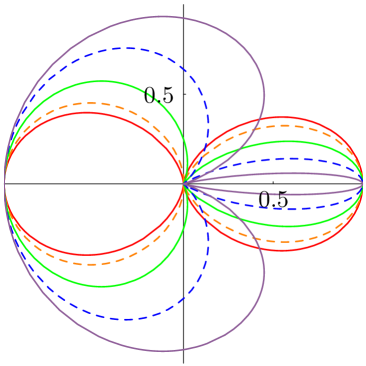
(a) (b)

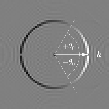
Figure 2: (a) Polar plot $[A(k\xi,\theta)]^{2}$ of the angular envelope function (15) for $k\xi=0.2\text{ (red)},0.5,1,2,5\text{ (violet)}$. The envelope is close to a dipole radiation (p-wave) pattern for sound waves $k\xi\ll 1$, and tends to an isotropic (s-wave) pattern for single-particle excitations $k\xi\gg 1$. In the intermediate regime, backscattering is favoured over forward scattering. (b) Density plot of $\text{Im}[\gamma_{{\boldsymbol{k}}^{\prime}}]$, the imaginary part of the Bogoliubov-transformed amplitude $\gamma_{{\boldsymbol{k}}^{\prime}}=u_{k^{\prime}}\delta\Psi_{{\boldsymbol{k}}^{\prime}}+v_{k^{\prime}}\delta\Psi^{*}_{-{\boldsymbol{k}}^{\prime}}$ from the numerical simulation of the GP equation. This figure is more distinct than Fig. 1(b), because the interference of Bogoliubov waves with $\pm{\boldsymbol{k}}^{\prime}$ is eliminated, and clearly shows the sign change across the scattering node $\theta_{0}$. Numerical parameters as in Fig. 1(b).

IV Back to the simulation

In order to confront these predictions with the numerical results, we first of all Bogoliubov-transform the numerically calculated momentum amplitude, $\gamma_{{\boldsymbol{k}}^{\prime}}=u_{k^{\prime}}\delta\Psi_{{\boldsymbol{k}}^{\prime}}{+}v_{k^{\prime}}\delta\Psi_{-{\boldsymbol{k}}^{\prime}}^{*}$, with the usual coefficients $u_{k}=(\epsilon_{k}+\epsilon^{0}_{k})/(2\sqrt{\epsilon_{k}\epsilon^{0}_{k}})$ and $v_{k}=(\epsilon_{k}-\epsilon^{0}_{k})/(2\sqrt{\epsilon_{k}\epsilon^{0}_{k}})$. In the corresponding plot of $\text{Im}[\gamma_{{\boldsymbol{k}}^{\prime}}]$, the imaginary part of the Bogoliubov-transformed amplitude, shown in Fig. 2(b), one can clearly see the amplitude sign change across the scattering node.

For a quantitative comparison with the numerical simulation, let now a single Bogoliubov excitation $\gamma_{{\boldsymbol{k}}}^{(0)}(t)=\gamma_{0}\exp\{-i\epsilon_{k}t/\hbar\}$ with wave vector ${\boldsymbol{k}}$ be scattered by the impurity potential as described by the effective Hamiltonian (12) and (13). In linear response (equivalent to the Born approximation of the corresponding quantum problem), the scattered amplitude $\gamma_{{\boldsymbol{k}}^{\prime}}^{(s)}(t)=\gamma_{{\boldsymbol{k}}^{\prime}}^{(s)}\exp\{-i\epsilon_{k}t/\hbar\}$ is given by $\gamma_{{\boldsymbol{k}}^{\prime}}^{(s)}=\gamma_{0}G_{0}(\epsilon_{k},k^{\prime})L^{-d/2}W_{{\boldsymbol{k}}^{\prime}{\boldsymbol{k}}}$, where $G_{0}(\epsilon,k)=\left[\epsilon-\epsilon_{k}+i0\right]^{-1}$ designates the retarded Green function of the free propagation described by (12). For a quantitative comparison with the numerical simulation in the finite system, one can coarse-grain over a $k$-space area $k\Delta\theta\Delta k$ around a point on the elastic circle at a given angle $\theta$. The analytical prediction for the coarse-grained imaginary part then reads

$$\text{Im}[\gamma^{(s)}_{\text{cg}}(\theta)]=-\pi\gamma_{0}\frac{\rho_{0}(\epsilon_{k})}{k}W(k,\theta)$$ (17)

in terms of the density of states per unit area, $\rho_{0}(\epsilon)=-1/(\pi L^{2})\sum_{\boldsymbol{k}}\text{Im}[G_{0}(\epsilon,k)]$. Coarse-graining similarly the numerical results on the elastic circle, we can plot together both amplitudes as function of the scattering angle $\theta$ at various wave vectors $k\xi$, see Fig. 3. The agreement is clearly very good, with residual numerical scatter around the analytical curves due to transients and boundary effects.

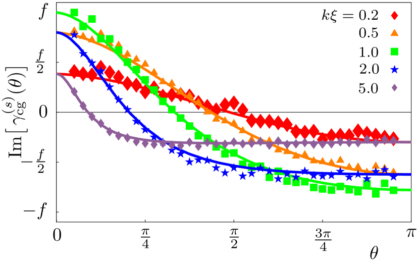
Figure 3: Coarse-grained elastic scattering amplitude (17) in units of $f=\gamma_{0}\,V_{0}/(8\xi\mu)$ for different values of $k\xi$, at fixed potential radius $kr_{0}=0.5$. Symbols: Results from numerical integration of the full GP equation. Solid curves: analytical prediction (17). With increasing $k$, the node moves to the left, according to (16). The overall amplitude has a maximum at $k\xi\approx 1$.

The overall magnitude of the scattering amplitude in Fig. 3 first grows and then decreases as $k\xi$ crosses from the sound-wave to the particle-regime, with most efficient scattering for wave vectors $k\xi\approx 1$. This behaviour results from two competing scalings: the Bogoliubov scattering amplitude $W(k,\theta)\propto\epsilon_{k}^{0}/\epsilon_{k}$ is proportional to $k$ for $k\xi\ll 1$ and saturates to a constant for $k\xi\gg 1$. The factor $\rho_{0}(\epsilon_{k})/k$ on the other hand is proportional to the inverse group velocity $(\partial k/\partial\epsilon_{k})$ that behaves like the constant $c^{-1}$ for sound waves $k\xi\ll 1$ and decreases as $k^{-1}$ for particles $k\xi\gg 1$. The product of both contributions in (17) therefore has limiting behaviour $k$ and $k^{-1}$, respectively, with a scattering maximum around the crossover $k\xi\approx 1$ from phonons to particles.

Note that Fig. 2(b) is much clearer than Fig. 1(b), because there Bogoliubov excitations with opposite $\pm{\boldsymbol{k}}^{\prime}$ interfere in the wave function densities $|\delta\Psi_{{\boldsymbol{k}}^{\prime}}|^{2}$. One may wonder why the superposition of nodes stemming from opposite wave vectors still gives a density dip as clear as in Fig. 1(b). In fact, in the single-particle case $k\xi\gg 1$ the ratio $v_{k}/u_{k}$ tends to zero such that only the node of one component is observed, whereas for sound waves $k\xi\ll 1$ both components contribute equally, but now with symmetric nodes at $\pm\frac{\pi}{2}$ that superpose exactly. This node robustness should facilitate the experimental observation.

V Experimental realisability

We propose our theoretical predictions to be experimentally tested following the numerical setup: A moderately strong, blue-detuned laser is focused perpendicularly through a 2D condensate Gorlitz2001 ; Hadzibabic2006 without depleting the condensate entirely. Then Bogoliubov excitations are imprinted optically Stamper-Kurn1999 ; Vogels2002 ; Steinhauer2002 ; Steinhauer2003 and observed in a subsequent time-of-flight measurement at time $t_{0}$. If necessary, the sensitivity to certain ${\boldsymbol{k}}$-components can be greatly improved using Bragg spectroscopy Brunello2000 ; Vogels2002 . In both cases, the total momentum distribution $|\Psi_{\boldsymbol{k}}(t_{0})|^{2}=|\Psi^{0}_{\boldsymbol{k}}+\delta\Psi_{\boldsymbol{k}}(t_{0})|^{2}$ at time $t_{0}$ is accessible. This is an oscillating quantity since the inverse Bogoliubov transformation $\delta\Psi_{\boldsymbol{k}}(t)=u_{k}\gamma_{\boldsymbol{k}}(t)-v_{k}\gamma_{-{\boldsymbol{k}}}^{*}(t)$ superposes components of Bogoliubov waves scattered into opposite directions with conjugate phases. The excitations $\delta\Psi_{\boldsymbol{k}}(t)$ live on the stationary background of the impurity-deformed condensate ground state $\Psi_{\boldsymbol{k}}^{0}\propto\tilde{v}_{\boldsymbol{k}}$ given by (7) such that the time-of-flight density would read $|\Psi_{\boldsymbol{k}}(t_{0})|^{2}=(\Psi^{0}_{\boldsymbol{k}})^{2}+2\Psi^{0}_{\boldsymbol{k}}\text{Re}\left[\delta\Psi_{\boldsymbol{k}}(t_{0})\right]+|\delta\Psi_{\boldsymbol{k}}|^{2}$. If a time average is performed, the linear oscillating term drops out, and the density $|\delta\Psi_{\boldsymbol{k}}|^{2}$ can be extracted by subtracting the ground-state density. Choosing an appropriate measurement time $t_{0}$ can reveal the amplitude $\text{Re}\left[\delta\Psi_{\boldsymbol{k}}(t_{0})\right]+{\mathcal{O}}(\delta\Psi^{2})$ on the smooth background $\Psi^{0}_{\boldsymbol{k}}$ with a better signal-to-noise ratio. The experiment could notably test the limits of validity of the weak-scattering linearisation and more generally the breakdown of mean-field behaviour.

VI Conclusions

A variational treatment has allowed us to derive a simple impurity-scattering Hamiltonian that governs the dynamics of Bogoliubov excitations in Bose superfluids in presence of a weak external potential. Remarkably, the single-scattering amplitude factorises into the impurity part and an angular envelope that describes the continuous transition from wave to particle behaviour as function of excitation momentum. Due to this factorisation, the theory is independent of the actual shape of the potential and can also be employed to describe disordered systems. In particular, we plan to generalise recent results on the disorder-induced localisation of Bogoliubov excitations in 1D Bilas2006 ; Lugan2007a to higher dimensions. Especially the 2D case promises to be interesting, because this is the lower critical dimension for the Anderson model of noninteracting particles in a random potential Abrahams1979 .

- (1) F. Dalfovo, S. Giorgini, L. P. Pitaevskii, and S. Stringari, “Theory of Bose-Einstein condensation in trapped gases”, Rev. Mod. Phys 71, 463 (1999).
- (2) Z. Hadzibabic, P. Krüger, M. Cheneau, B. Battelier, and J. Dalibard, “Berezinskii-Kosterlitz-Thouless crossover in a trapped atomic gas”, Nature 441, 1118 (2006).
- (3) P. Krüger, Z. Hadzibabic, and J. Dalibard, “Critical point of an interacting two-dimensional atomic Bose gas”, Phys. Rev. Lett. 99, 040402 (2007), eprint arXiv:cond-mat/0703200.
- (4) T. Giamarchi and H. J. Schulz, “Localization and interaction in one-dimensional quantum fluids”, EPL (Europhysics Letters) 3, 1287 (1987).
- (5) M. P. A. Fisher, P. B. Weichman, G. Grinstein, and D. S. Fisher, “Boson localization and the superfluid-insulator transition”, Phys. Rev. B 40, 546 (1989).
- (6) D. Belitz, T. R. Kirkpatrick, and T. Vojta, “How generic scale invariance influences quantum and classical phase transitions”, Rev. Mod. Phys. 77, 579 (2005), eprint arXiv:cond-mat/0403182.
- (7) V. Gurarie and J. T. Chalker, “Bosonic excitations in random media”, Phys. Rev. B 68, 134207 (2003), eprint arXiv:cond-mat/0305445.
- (8) A. Posazhennikova, “Colloquium: Weakly interacting, dilute Bose gases in 2D”, Rev. Mod. Phys. 78, 1111 (2006), eprint arXiv:cond-mat/0506034.
- (9) D. M. Stamper-Kurn, et al., “Excitation of phonons in a Bose-Einstein condensate by light scattering”, Phys. Rev. Lett. 83, 2876 (1999).
- (10) J. M. Vogels, K. Xu, C. Raman, J. R. Abo-Shaeer, and W. Ketterle, “Experimental observation of the Bogoliubov transformation for a Bose-Einstein condensed gas”, Phys. Rev. Lett. 88, 060402 (2002), eprint arXiv:cond-mat/0109205.
- (11) J. Steinhauer, R. Ozeri, N. Katz, and N. Davidson, “Excitation spectrum of a Bose-Einstein condensate”, Phys. Rev. Lett. 88, 120407 (2002), eprint arXiv:cond-mat/0111438.
- (12) J. Steinhauer, et al., “Bragg spectroscopy of the multibranch Bogoliubov spectrum of elongated Bose-Einstein condensates”, Phys. Rev. Lett. 90, 060404 (2003).
- (13) M. C. W. van Rossum and T. M. Nieuwenhuizen, “Multiple scattering of classical waves: microscopy, mesoscopy, and diffusion”, Rev. Mod. Phys. 71, 313 (1999), eprint arXiv:cond-mat/9804141.
- (14) L. Pitaevskii and S. Stringari, Bose-Einstein condensation, Clarendon Press, Oxford (2003).
- (15) R. C. Kuhn, C. Miniatura, D. Delande, O. Sigwarth, and C. A. Müller, “Localization of matter waves in two-dimensional disordered optical potentials”, Phys. Rev. Lett. 95, 250403 (2005).
- (16) R. C. Kuhn, O. Sigwarth, C. Miniatura, D. Delande, and C. A. Müller, “Coherent matter wave transport in speckle potentials”, New J. Phys. 9, 161 (2007), eprint arXiv:cond-mat/0702183.
- (17) L. D. Landau and E. M. Lifschitz, Fluid Mechanics, chapter 8, § 78, Butterworth Heinemann (2004).
- (18) S. Giorgini, L. Pitaevskii, and S. Stringari, “Effects of disorder in a dilute Bose gas”, Phys. Rev. B 49, 12938 (1994), eprint arXiv:cond-mat/9402015.
- (19) L. Sanchez-Palencia, “Smoothing effect and delocalization of interacting Bose-Einstein condensates in random potentials”, Phys. Rev. A 74, 053625 (2006), eprint arXiv:cond-mat/0609036.
- (20) K. Huang and H.-F. Meng, “Hard-sphere Bose gas in random external potentials”, Phys. Rev. Lett. 69, 644 (1992).
- (21) A. Görlitz, et al., “Realization of Bose-Einstein condensates in lower dimensions”, Phys. Rev. Lett. 87, 130402 (2001).
- (22) A. Brunello, F. Dalfovo, L. Pitaevskii, and S. Stringari, “How to measure the Bogoliubov quasiparticle amplitudes in a trapped condensate”, Phys. Rev. Lett. 85, 4422 (2000), eprint arXiv:cond-mat/0007125.
- (23) N. Bilas and N. Pavloff, “Anderson localization of elementary excitations in a one dimensional Bose-Einstein condensate”, Eur. Phys. J. D 40, 387 (2006), eprint arxiv:cond-mat/0602622.
- (24) P. Lugan, D. Clément, P. Bouyer, A. Aspect, and L. Sanchez-Palencia, “Anderson localization of Bogolyubov quasiparticles in interacting Bose-Einstein condensates”, Phys. Rev. Lett. 99, 180402 (2007), eprint arXiv:0707.2918.
- (25) E. Abrahams, P. W. Anderson, D. C. Licciardello, and T. V. Ramakrishnan, “Scaling theory of localization: Absence of quantum diffusion in two dimensions”, Phys. Rev. Lett. 42, 673 (1979).