Magnetic edge states in graphene in nonuniform magnetic fields

Abstract

We theoretically study electronic properties of a graphene sheet on $xy$ plane in a spatially nonuniform magnetic field, $B=B_{0}\hat{z}$ in one domain and $B=B_{1}\hat{z}$ in the other domain, in the quantum Hall regime and in the low-energy limit. We find that the magnetic edge states of the Dirac fermions, formed along the boundary between the two domains, have features strongly dependent on whether $B_{0}$ is parallel or antiparallel to $B_{1}$. In the parallel case, when the Zeeman spin splitting can be ignored, the magnetic edge states originating from the $n=0$ Landau levels of the two domains have dispersionless energy levels, contrary to those from the $n\neq 0$ levels. Here, $n$ is the graphene Landau-level index. They become dispersive as the Zeeman splitting becomes finite or as an electrostatic step potential is additionally applied. In the antiparallel case, the $n=0$ magnetic edge states split into electron-like and hole-like current-carrying states. The energy gap between the electron-like and hole-like states can be created by the Zeeman splitting or by the step potential. These features are attributed to the fact that the pseudo-spin of the magnetic edge states couples to the direction of the magnetic field. We propose an Aharonov-Bohm interferometry setup in a graphene ribbon for experimental study of the magnetic edge states.

I Introduction

Graphene, a two-dimensional (2D) honeycomb lattice of carbons, has attracted much attention, because of its unusual electronic properties. In the low-energy regime, electrons near the two inequivalent valleys, $K$ and $K^{\prime}$, of its electronic structure can be described by massless Dirac fermionsSemenoff ; Haldane and exhibit half-integer quantum Hall effects,Novoselov ; Zhang in contrast to the quantum Hall effect of the conventional 2D electrons formed in semiconductor heterostructures.Chakraborty The long phase coherence length and mean free path, of micrometer order, measuredBerger ; Miao in high-quality graphenes indicate potential applications of a graphene ribbon to coherent nanodevices.

On the other hand, the electron properties of the conventional 2D systems have been investigated in the presence of spatially nonuniform magnetic fields. The nonuniform fields can cause the formation of charateristic current-carrying edge statesMints ; Muller along the region of field gradient, which correspond to the semi $\vec{\nabla}B\times\vec{B}$ drift motion. These states have been referedSim as magnetic edge states in the analogy to the edge states,Halperin corresponding to the $\vec{E}\times\vec{B}$ drift, along sample boundaries. Their features have been studied experimentally.Nogaret The nonuniform fields can form various magnetic structures such as magnetic steps,Peeters1 ; Badalyan ; Reijniers1 magnetic quantum dots,Sim ; Reijniers2 ; Novoselov2 magnetic rings,Kim magnetic superlattices,Carmona ; Ye ; Ibrahim etc, and play a role of characteristic barriers and resonators of electron transport,Matulis ; Sim2 which properties are very different from those formed by electrostatic gate potential.

A graphene sheet may provide a good experimental system for studying the effects of the nonuniform magnetic fields as a nonuniform-field configuration can be effectively generated by applying a uniform field to a curved sheet.Leadbeater In addition, the Dirac fermions in graphene can have interesting properties under the nonuniform fieldsMartino , which may be different from those of the magnetic edge states in the conventional 2D systems, since the Dirac fermions have electron-like, zero-mode, and hole-like Landau levels, as well as the pseudo-spins representing the two sub-lattice sites of the honeycomb lattice. Therefore, it may be valuable to study the electron properties of graphene in a nonuniform magnetic field, which is the aim of the present work.

In this theoretical work, we study the electronic structures of a graphene sheet (on $xy$ plane) in a spatially nonuniform magnetic field of step shape, $\vec{B}=B_{0}\hat{z}$ for $x<0$ and $\vec{B}=B_{1}\hat{z}$ for $x>0$, in the integer quantum Hall regime, based on a noninteracting-electron approach. By solving the Dirac equation, we first investigate the low-energy properties of the magnetic edge states formed along the boundary ($x=0$) between the two domains with different fields $B_{0}$ and $B_{1}$, when the Zeeman effect is negligible. They are found to strongly depend on whether $B_{0}$ is parallel or antiparallel to $B_{1}$. In the palallel case of $\gamma\equiv B_{1}/B_{0}>0$, the magnetic edge states originating from the $n=0$ Landau levels of the two domains are dispersionless, contrary to those from the $n\neq 0$ levels, where $n$ is the Landau level index. In the antiparallel case of $\gamma<0$, the $n=0$ magnetic edge states split into electron-like and hole-like levels near the boundary. These features, which are absent in the magnetic edge states of the conventional 2D electrons, are attributed to the fact that the pseudo-spin of the magnetic edge states couples to the direction of the magnetic field. On the other hand, the features of the $n\neq 0$ magnetic edge states are similar to those of the conventional cases.

We further study the magnetic edge states in the presence of an additional electrostatic step potential, $V(x)=V_{0}$ for $x<0$ and $V(x)=V_{1}$ for $x>0$. For $\gamma>0$, the $n=0$ magnetic edge states become dispersive, while for $\gamma<0$ an energy gap becomes created around the bipolar region in the spectrum of the magnetic edge states. Similar features can be found when the Zeeman spin splitting is finite, because in the nonuniform field of step shape the Zeeman effect behaves as the step potential.

Finally, we suggest an interferometry setup formed in a graphene ribbon for experimental study. In this setup, the magnetic edge states can provide partial paths of a full Aharonov-Bohm interference loop, therefore the properties of the magnetic edge states such as the gap of their energy spectra can be investigated. We numerically calculate the transmission probability through the setup by using the tight-binding method and the Green function technique.Meir ; Datta ; Sim3 The results are consistent with the features of the magnetic edge states obtained by solving the Dirac equation. We also derive the transmission probability, based on the scattering matrix formalism, and use it to analyze the numerical results.

This paper is organized as follows. The magnetic edge states are studied without and with the electrostatic step potential in Secs. II and III, respectively. The Zeeman spin splitting is considered in Sec. IV, and the graphene interferometry is suggested and investigated in Sec. V. In Sec. VI, this work is summarized. Throughout this work, we ignore the intervalley mixing due to the nonuniform field, the validity of which is discussed in Appendix A. In Appendix B we derive the transmission probability, which may be applicable to other graphene interferometry setups with slight modification.

II Magnetic edge states

We consider a graphene sheet (on $xy$ plane) in the nonuniform magnetic field of the step configuration,

$$\vec{B}(x)=\left\{\begin{array}[]{ll}B_{0}\hat{z},&\hbox{$x<0$}\\ B_{1}\hat{z},&\hbox{$x>0$}\end{array}\right.$$ (3)

in the integer quantum Hall regime. Without loss of generality, $B_{0}$ is chosen to be positive, and $\gamma\equiv B_{1}/B_{0}$ is either positive or negative. This configuration may be realized with field gradient $dB/dx$ less than $10^{4}\,\,\,\textrm{T}\cdot\textrm{{\AA}}^{-1}$ and with not-too-strong field strengths $B_{0}$ and $|B_{1}|$ (less than, e.g., 100 T). In this case, the mixing between the $K$ and $K^{\prime}$ valleys due to the nonuniform field can be ignored (see Appendix A), and the electrons in each valley can be seperately described by the Dirac equation,

$$[v\vec{\sigma}_{J}\cdot\vec{\Pi}+V(x)]\Psi_{J} = E\Psi_{J},$$ (4)

in the low-energy approximation. Here, $J\in\{K,K^{\prime}\}$ is the valley index, $v=\sqrt{3}at/(2\hbar)\sim 10^{6}\,\,\textrm{m}\cdot\textrm{s}^{-1}$, $a$ is the lattice constant of graphene, $t$ is the hopping energy between two nearest neighbor sites, $\vec{\sigma}_{K}=(\sigma_{x},\sigma_{y})$ and $\vec{\sigma}_{K^{\prime}}=(-\sigma_{x},\sigma_{y})$ are constructed by the Pauli matrices, $\vec{\Pi}\equiv\vec{p}+e\vec{A}$, $\vec{p}$ is the momentum measured relative to the valley center ($K$ or $K^{\prime}$ point), $\vec{A}$ is the vector potential, and $e(>0)$ is the electron charge. The electrostatic potential $V(x)$ applied to the sheet must be a smoothly varying function of $x$. The detailed form of $V(x)$ will be specified in Sec. III. The components of the pseudo-spinor $\Psi_{J}$ represent the wave functions of the two sub-lattice sites (denoted by $A$ and $B$ hereafter) of a unit cell of graphene. The Dirac equations for the $K$ and $K^{\prime}$ valleys are connected to each other by a unitary transformation $U=\sigma_{y}$. This feature leads that the two equations have the same energy levels and that their wave functions have the relation, $\Psi_{K^{\prime}}=U\Psi_{K}$. Therefore, it is enough to solve the Dirac eqaution for the $K$ valley only.

Before studying the nonuniform-field cases, we briefly discuss the case of a uniform magnetic field with strength $B$. In this case, the Landau levels are foundNovoselov to be

$$E_{n}=\textrm{Sgn}(n)v\sqrt{2|n|\hbar eB},$$ (5)

where $n=0,\pm 1,\pm 2,\cdots$ is the Landau level index. The levels with $n>0$ are often refered as electron-like, while those with $n<0$ as hole-like. In fact, one can obtain the Landau levels from the square of the Dirac Hamiltonian,

$$E_{n}^{2}=2\hbar ev^{2}B(m+1/2\pm 1/2)$$ (6)

for the $K$ valley, with $|n|=m+1/2\pm 1/2$ and $m=0,1,2,\cdots$. For later discussion, it is worthwhile to analyze $E_{n}^{2}$. The harmonic term with $B(m+1/2)$ is nothing but the Landau level of the conventional 2D electrons, while the next term $\pm B/2$ can be interpreted as the effective Zeeman effect of the pseudo-spin; $B/2$ for pseudo-spin up and $-B/2$ for down. Each Landau level with $n\neq 0$ is composed of the pseudo-spin up (with $m=|n|-1$) and pseudo-spin down (with $m=|n|$) states, while the $n=0$ level comes only from the pseudo-spin down (up) states with $m=0$ in the $K$ ($K^{\prime}$) valley. The $n=0$ level is independent of $B$ as the harmonic and effective Zeeman terms exactly cancel each other.

Turning back to the nonuniform field in Eq. (3), we consider the case without electrostatic potential, $V(x)=0$, in this section. We choose the vector potential as $\vec{A}(x)=B_{0}x\hat{y}$ for $x<0$ and $\vec{A}(x)=B_{1}x\hat{y}$ for $x>0$. This choice of $\vec{A}$ is useful, as the solution of Eq. (4) for the $K$ valley can be written as $\Psi_{K}^{\dagger}(x)=e^{-iky}\Phi^{\dagger}(x)=e^{-iky}(\phi^{\ast}_{A}(x),\phi^{\ast}_{B}(x))$, where $\phi_{j}$ is the wave function of the sub-lattice site $j\in\{A,B\}$ and $\hbar k$ is the eigenvalue of $p_{y}$. Hereafter we will measure energy and length in units of $E_{1}(\equiv\sqrt{2\hbar v^{2}eB_{0}})$ and $l_{B}(\equiv\sqrt{\hbar/(eB_{0})})$, where $l_{B}$ and $E_{1}$ are the magnetic length and the energy gap between the $n=0$ and $n=1$ Landau levels, respectively, of the bulk region with $B_{0}$; in these units, the Landau levels are $\sqrt{n}$ at $x\ll-1$ while $\textrm{Sgn}(n)\sqrt{|\gamma|n}$ at $x\gg 1/\sqrt{|\gamma|}$. Then the equation for $\phi_{j=A,B}$ is found to be

$$-\frac{d^{2}\phi_{j,k}(x)}{dx^{2}}+2[V^{j}_{\rm eff}(x,k)-E^{2}_{n,k}]\phi_{j,k}(x)=0.$$ (7)

The effective potentialSim $V_{\rm eff}^{j}$ is harmonic,

$$V^{j}_{\rm eff}(x,k)=\left\{\begin{array}[]{ll}\frac{1}{2}(x+k)^{2}+s_{j}\frac{1}{2},&\hbox{$x<0$}\\ \\ \frac{1}{2}(\gamma x+k)^{2}+s_{j}\frac{\gamma}{2},&\hbox{$x>0,$}\end{array}\right.$$ (8)

where $s_{j=A}=1$ and $s_{j=B}=-1$. The equation (7) has the form of the usual Schrödinger equation with potential $V_{\rm eff}^{j}$ and eigenvalue $E^{2}_{n,k}$. Therefore, $V_{\rm eff}^{j}$ is useful for understanding $\phi_{j,k}(x)$ and $E_{n,k}$. The form of $V_{\rm eff}^{j}$ in Eq. (8) shows that the pseudo-spin ($s_{j}$) couples to the direction ($\gamma$) of the magnetic field.

The solution $\phi_{j,k}^{<}$ of Eq. (7) for $x<0$ can be expressed in terms of the parabolic cylinder functionsLebedev $D_{\nu}(z)$ as

$$\left(\begin{array}[]{c}\phi^{<}_{A,k}\\ \phi^{<}_{B,k}\end{array}\right)\propto\left(\begin{array}[]{c}iED_{E^{2}-1}(-\sqrt{2}(x+k))\\ D_{E^{2}}(-\sqrt{2}(x+k))\end{array}\right).$$ (9)

On the other hand, for $x>0$, the solution $\phi_{j,k}^{>}$ is found to be dependent on the sign of $\gamma$, i.e., on whether $B_{1}$ is either parallel or antiparallel to $B_{0}$, as for $\gamma>0$

$$\left(\begin{array}[]{c}\phi^{>}_{A,k}\\ \phi^{>}_{B,k}\end{array}\right)\propto\left(\begin{array}[]{c}-i\frac{E}{\sqrt{\gamma}}D_{\frac{E^{2}}{\gamma}-1}(\sqrt{2\gamma}(x+\frac{k}{\gamma}))\\ D_{\frac{E^{2}}{\gamma}}(\sqrt{2\gamma}(x+\frac{k}{\gamma}))\end{array}\right),$$ (10)

and for $\gamma<0$

$$\left(\begin{array}[]{c}\phi^{>}_{A,k}\\ \phi^{>}_{B,k}\end{array}\right)\propto\left(\begin{array}[]{c}D_{\frac{E^{2}}{|\gamma|}}(\sqrt{2|\gamma|}(x+\frac{k}{\gamma}))\\ -i\frac{E}{\sqrt{|\gamma|}}D_{\frac{E^{2}}{|\gamma|}-1}(\sqrt{2|\gamma|}(x+\frac{k}{\gamma}))\end{array}\right).$$ (11)

The energy eigenvalue $E_{n,k}$ can be obtained under the boundary condition of the continuity of the wave functions in Eqs. (9)-(11) at $x=0$. For the two cases of $\gamma=2$ and $\gamma=-1$, $E_{n,k}$ is drawn in Fig. 1. These two specific cases of $\gamma$ are enough to understand the characteristics of the magnetic edge states.

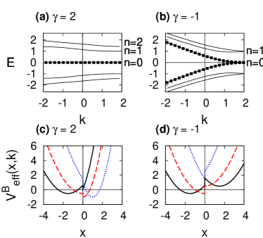
Figure 1: (Color online) Upper panels: Energy spectra $E_{n,k}$ for (a) $\gamma=2$ and (b) $\gamma=-1$. The energy levels of the $n=0$ magnetic edge states are highlighted by the filled squares. For $\gamma>0$, the $n=0$ levels are dispersionless while they split into electron-like and hole-like levels for $\gamma<0$. Lower panels: Effective potential $V^{j=B}_{\rm eff}(x,k)$ in Eq.(8) for (c) $\gamma=2$ and (d) $\gamma=-1$. Different values of $k=1.5$ (solid line), 0 (dashed), -2 (dotted) are chosen. Energy and length are measured in units of $E_{1}(\equiv\sqrt{2\hbar v^{2}eB_{0}})$ and $l_{B}(\equiv\sqrt{\hbar/(eB_{0})})$, respectively.

The energy levels strongly depend on whether $B_{1}$ is parallel or antiparallel to $B_{0}$. In the parallel case of $\gamma>0$, for each $n$ the energy levels gradually change from $\textrm{Sgn}(n)\sqrt{|n|}$ to $\textrm{Sgn}(n)\sqrt{\gamma|n|}$ as $k$ decreases from positive to negative values [see the $\gamma=2$ case in Fig. 1(a)]. This feature can be understood from the effective potential [see Eq. (8) and Fig. 1(c)]. As $k$ increases from negative to positive values, the bottom of $V_{\rm eff}^{j}(x)$ moves from the region with $B_{1}$ to that with $B_{0}$, passing the boundary $x=0$ around $k=0$. Therefore, for $k\ll 0$, the eigenstates have the Landau levels $\textrm{Sgn}(n)\sqrt{\gamma|n|}$ and localize around $x=-k/\gamma$ (in the unit of $\l_{B}$), while for $k\gg 0$, they have $\textrm{Sgn}(n)\sqrt{|n|}$ and localize around $x=-k$. Around $k=0$, the two levels of $\textrm{Sgn}(n)\sqrt{\gamma|n|}$ and $\textrm{Sgn}(n)\sqrt{|n|}$ connect smoothly and the corresponding states are localized around $x=0$. These states have been calledSim magnetic edge states and they can carry current along the boundary $x=0$.

Contrary to the corresponding states in the conventional 2D systems, the magnetic edge states in graphene have the following different features for $\gamma>1$. First, the edge states with $n>0$ behave as electrons, with dispersion $dE_{n}/dk<0$ while those with $n<0$ as holes with $dE_{n}/dk>0$. Second, the edge states with $n=0$ are dispersionless and carry no current, regardless of $\gamma(>0)$. These features come from the nature of the Dirac fermions. Especially, the second one can be understood from the fact that for $\gamma>0$, the effective Zeeman and harmonic contributions to $E^{2}_{n=0}$ cancel each other in the both sides of $x=0$, as discussed around Eq. (6) and as shown in the term of $V_{\rm eff}^{j}$ representing the coupling of pseudo-spin to field direction [see Eq. (8)]. The case of $0<\gamma<1$ can be understood in a similar way.

Next, we discuss the case of $\gamma<0$, which is very different from the $\gamma>0$ case [see Fig. 1(b)]. For large positive $k$, the eigenstates have the Landau levels of $\textrm{Sgn}(n)\sqrt{|n|}$ or $\textrm{Sgn}(n)\sqrt{|\gamma n|}$, while for large negative $k$ $(\ll 0)$, their energy either increases (showing electron-like behavior) or decreases (hole-like). This feature can be understood from $V^{j}_{\rm eff}(x,k)$. As shown in Fig. 1(d), for large positive $k$, the two local harmonic wells of $V^{j}_{\rm eff}(x,k)$ occur far from the boundary of $x=0$, resulting in the Landau levels localized in each well. As $k$ decreases to negative values, the two local wells move toward $x=0$ and become to merge into a single well (not harmonic anymore) at $x=0$, and then the bottom of the merged well increases. Therefore, the eigenstates with $k\lesssim 0$ are magnetic edge states localized at $x=0$ and they can carry current along $x=0$. They are either electron-like ($dE_{n\geq 0}/dk<0$) or hole-like ($dE_{n\leq 0}/dk>0$). One can estimate their group velocity for $k\ll 0$ as $(1/\hbar)dE_{n}/dk\sim\pm v$ from the minimum value of the merged well of $V_{\rm eff}^{B}$, where $+(-)$ stands for the hole(electron)-like states. In this case of $\gamma<0$, where the magnetic fields $B_{0}$ and $B_{1}$ are antiparallel, the eigenstates in $n\neq 0$ Landau levels correspond to classical motions, so called snake orbitsMints ; Muller ; Sim ; Badalyan , while those in the $n=0$ level have no clear correspondence to classical motions as they have both electron and hole characters.

For $\gamma<0$, the effective Zeeman contribution to $E_{n}^{2}$ has the opposite sign between the domains of $x>0$ and $x<0$, as shown in Eq. (8). This coupling of pseudo-spin to field direction causes an energy barrier at $x=0$; for example, a pseudo-spin down state has larger effective Zeeman contribution at $x>0$ than at $x<0$. As a result, as $k$ decreases, the magnetic edge state becomes more confined around $x=0$ due to the effective-Zeeman barrier. This pseudo-spin feature, which enhances the splitting into electron-like and hole-like states, is absent in the magnetic edge states of the conventional 2D electrons.

III Magnetic edge states in an electrostatic step potential

In this section, we consider an additional electrostatic potential $V(x)$ of step shape,

$$V(x)=\left\{\begin{array}[]{ll}V_{0},&\hbox{$x<0$}\\ V_{1},&\hbox{$x>0$},\end{array}\right.$$ (12)

to the nonuniform magnetic field in Eq. (3). Here $V_{0}$ and $V_{1}$ are constant. This potential gives rise to characteristic modification of the $n=0$ magnetic edge states, such as the creation of energy gap for $\gamma<0$, as will be seen below. Moreover, the modification is directly applicable to the case where the Zeeman spin splitting is finite, as will be studied in Sec. IV.

Figure 2: The same as in Fig. 1 but in the presence of the step potential $V(x)$ with $V_{0}=0$ and $V_{1}=0.5$. For $\gamma=-1$, the energy levels are labeled by $n_{L}$ and $n_{R}$, which are the indices of the Landau levels localized at $x\ll-1$ and at $x\gg 1/\sqrt{|\gamma|}$, respectively (see text). The $n=0$ levels become dispersive for $\gamma>0$ while the energy gap opens between electron-like ($n_{R}=0$) and hole-like levels ($n_{L}=0$) for $\gamma<0$.

The step potential $V(x)$ is assumed to be smoothly varying in the length scale of the lattice constant $a$. Then, we can still ignore the intervalley mixing and solve the Dirac equation in Eq. (4) in the same way as above. In Fig. 2, choosing $V_{0}=0$ and $V_{1}=0.5$ (in the units of $E_{1}$ and $l_{B}$), we draw the energy spectra of the magnetic edge states for $\gamma=2$ and $\gamma=-1$.

The features of the energy spectra are discussed below. For $\gamma>0$, the eigenstates with large positive (negative) $k$ have the Landau levels shifted by $V_{0}$ ($V_{1}$) and do not carry current, while the magnetic states around $k=0$ have the energy smoothly connecting the Landau levels of the large positive and negative $k$’s. We point out that the $n=0$ magnetic edge states carry current due to the potential step $V(x)$. On the other hand, for $\gamma<0$, the eigenstates with large positive $k$ have the Landau levels shifted by $V_{0}$ or $V_{1}$, depending on whether they are localized in the bulk region of $x<0$ or $x>0$. For convenience, we introduce the Landau-level indices $n_{L}$ and $n_{R}$ for those localized in $x<0$ and in $x>0$, respectively. In this case, the energy levels with $n=0$ split, opening the energy gap between the electron-like and hole-like magnetic edge states, in contrary to the case without the step potential. For $\gamma=-1$ and $V_{1}-V_{0}=0.5$, the gap size is the same as the step height $V_{1}-V_{0}$.

We further study the energy gap with varying the height $V_{1}-V_{0}$ for $\gamma=-1$. In Fig. 3, we choose $V_{1}-V_{0}=1.5$, which is larger than the energy spacing between the $n=0$ and $n=1$ Landau levels, in contrary to the case of Fig. 2(b) where the height (= 0.5) is smaller. In this case, the energy gap of the magnetic edge states occurs between the $n_{L}=1$ and $n_{R}=-1$ Landau levels. Moreover, the gap size is no longer the same as the step height, but corresponds to the energy difference (= 0.5) between the $n_{L}=1$ and $n_{R}=-1$ levels.

Figure 3: The same as in Fig. 2(b) but with $(V_{0},V_{1})=(0,1.5)$.

The above feature can be understood as follows. For $\gamma=-1$, the effective Hamiltonian in Eq. (4) is odd under the inversion operator $\mathcal{R}_{\rm inv}$, $\mathcal{R}_{\rm inv}\vec{x}=-\vec{x}$,

$$\mathcal{R}_{\rm inv}\big{[}v\vec{\sigma}_{J}\cdot\vec{\Pi}+V(x)-\frac{V_{0}+V_{1}}{2}\big{]}\mathcal{R}_{\rm inv}\mathcal{R}_{\rm inv}\Psi_{J}$$ (13)

$$= -\big{[}v\vec{\sigma}_{J}\cdot\vec{\Pi}+V(x)-\frac{V_{0}+V_{1}}{2}\big{]}\mathcal{R}_{\rm inv}\Psi_{J}$$

$$= (E-\frac{V_{0}+V_{1}}{2})\mathcal{R}_{\rm inv}\Psi_{J}.$$

This property is consistent with the facts that the gap center is located at $E_{c}\equiv(V_{0}+V_{1})/2$ and that the gap size is determined by the energy difference between the Landau levels just below and above $E_{c}$. Similarly to the case in Fig. 1, it can be also understoodEFFECTIVE from $V_{\rm eff}^{j}$ that the states with $E>E_{c}$ are electron-like while those with $E<E_{c}$ are hole-like.

IV Zeeman splitting of the magnetic edge states

So far, we have ignored the spin degree of freedom. Recently, Abanin, Lee, and Levitov discussedAbanin that in graphene the Zeeman splitting can be smaller than the Landau energy gap only by the factor of about $10^{-1}$, due to the exchange interaction, and that it can play an important role in the edge-channel transport in the quantum Hall regime. In this section, we discuss the effect of the Zeeman splitting on the magnetic edge states.

Figure 4: Schematic spin-dependent energy dispersion of the $n=0$ magnetic edge states in the presence of the Zeeman splitting, 2 $|V_{s}^{\rm Z}|=0.2$. We choose the parameters $(\gamma,V_{0},V_{1})$ as (a) (2,0,0), (b) (2,-0.2,0.2), (c) (-1,0,0), (d) (-1,-0.2,0.2).

In the nonuniform field $B(x)$ in Eq. (3), the Zeeman splitting behaves as a spin-dependent step potential,

$$V^{\rm Z}_{s}(x)=s\Delta_{Z}B(x),$$ (14)

where $\Delta_{\rm Z}=g^{*}\mu_{B}/E_{1}$, $s=1/2$ ($s=-1/2$) for spin-up (down) electrons, and $\mu_{B}$ is the Bohr magneton. The exchange enhancementAbanin of the $g$-factor can be taken into account in $g^{*}$. We assume that $V^{\rm Z}_{s}\ll 1$ for convenience.

The Zeeman splitting can be considered as the spin-dependent shift of the step potential, $V(x)\to V(x)+V^{\rm Z}_{s}(x)$. The resulting magnetic edge states can be easily understand from the features discussed in Sec. III. In Fig. 4, we draw schematic energy dispersions of the $n=0$ magnetic edge states; the extension to $n\neq 0$ states is trivial. For $\gamma>0$, the $n=0$ states are dispersive near $x=0$, as shown in Figs. 4(a) and (b). The energy difference between the spin-up and down states varies from $\gamma\Delta_{\rm Z}$ to $\Delta_{\rm Z}$ as $k$ increases. And, the average value of the spin-up and down energy levels is shifted by $V_{0}$ ($V_{1}$) at large positive (negative) $k$. On the other hand, for $\gamma<0$, the energy gap of the $n=0$ magnetic edge states exists even without the electrostatic step potential [see Fig. 4(c)]. For both the cases of $\gamma>0$ and $\gamma<0$, the sign of the drift velocity ($\sim dE/dk$) is either positive or negative, depending on $\Delta_{\rm Z}$, $V_{0}$, and $V_{1}$. These spin-split dispersions show that spin-polarized current can emerge between two magnetic domains.

V Graphene interferometry

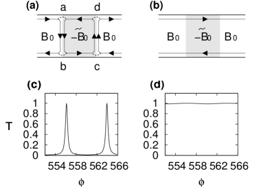
Figure 5: Upper panel: Schematic diagram of a graphene-ribbon interferometry, which consists of the left (with magnetic field $B_{0}$), middle (with $-\tilde{B}_{0}$), and right (with $B_{0}$) regions. There is one edge channel along the ribbon edges, while there can be magnetic edge states along the left and right boundaries, $\bar{ab}$ and $\bar{cd}$, of the middle region, depending on the energy of the states and the field configuration of ($B_{0}$, $-\tilde{B}_{0}$). In (a), there appear two magnetic edge states along each boundary, and thus the Aharonov-Bohm interference, while no state and no interference exists in (b). Lower panel: Aharonov-Bohm effect in the transmission $T$ through the interferometry, as a function of the Aharonov-Bohm flux $\phi$. The case of (a) is plotted in (c), while that of (b) in (d).

In this section, we propose an interferometry setup for studying magnetic edge states in a graphene ribbon. We focus on the case of $\gamma=-1$ in Fig. 2(b) and demonstrate that the energy gap of the magnetic edge states can be directly studied by observing the Aharonov-Bohm interference of the setup. The interferometry setup is useful as well for the other cases of $\gamma$.

We consider a ribbon with armchair edge; a setup with zigzag edge will show a similar result. The ribbon consists of three parts, the current source in the left, the middle scattering region, and the drain in the right. A nonuniform magnetic field is applied such that $B=B_{0}\hat{z}$ in the source and drain while $B=\tilde{B}_{0}\hat{z}\simeq-B_{0}\hat{z}$ in the middle region (see Fig. 5). At the same time, a constant electrostatic potential $V_{0}=0$ is applied in the source and drain while $V_{1}=0.5$ in the middle region. Then, the magnetic edge states form along the left and right boundaries $\bar{ab}$ and $\bar{cd}$ of the middle region, while along each boundary of the ribbon, there is one edge channel, which is formed as a mixture of the contribution of the $K$ and $K^{\prime}$ valleys.Brey The magnetic edge states are the same as those studied in Fig. 2(b), when their position separates from the ribbon edge by more than the scale of magnetic length, $l_{B}\equiv\sqrt{\hbar/(eB_{0})}$, so that the overlap between the magnetic edge states and the ribbon-edge channels is negligible. Note that at each of the scattering points $a$-$d$ in Fig. 5(a), the number of the incoming channels is the same as that of the outgoing channels, so that the current is conserved.

The formation of the magnetic edge states depends on energy. In the energy range $\in[0.5,1]$ of Fig. 2(b), where each valley supports only one magnetic edge channel, one has the edge-channel transport shown in Fig. 5(a). In this case, there appears an Aharonov-Bohm loop around the middle region, which is supported by the two counterpropagating edge channels along the upper and lower ribbon edges and by the magnetic edge states along the boundaries $\bar{ab}$ and $\bar{cd}$. As a function of $\tilde{B}_{0}$, one can observe the Aharonov-Bohm interference in the transmission through the setup. On the other hand, in the energy range $\in[0,0.5]$, where there is no magnetic edge state along $\bar{ab}$ and $\bar{cd}$ [see Fig. 5(b)], no Aharonov-Bohm interference can be observed. Therefore, the Aharonov-Bohm loop can be formed, depending on whether the magnetic edge channels exist along the boundaries $\bar{ab}$ and $\bar{cd}$. This property allows one to measure the gap of the magnetic edge states by varying the energy of the incoming edge channel and by modulating $\tilde{B}_{0}$.

We confirm the above proposal numerically by calculating the transmission probability $T(E)$ through the setup, using the tight-binding methodBrey2 and the Green’s function approach.Meir ; Datta Here we skip the details of the method and instead refer Refs. Sim2 ; Sim3 . The effect of the magnetic field is taken into account by the Peierls phase. The strength of $B_{0}$ is set to be about 800 T. At the boundaries $\bar{ab}$ and $\bar{cd}$, the magnetic field spatially varies linearly from $B_{0}$ to $\tilde{B}_{0}$ over the length scales of $3l_{B}$. We choose the ribbon width $|\bar{ab}|$ and the width $|\bar{bc}|$ of the middle region as about $15l_{B}$ and $30l_{B}$, respectively, so that we can ignore the overlap between the edge channels propagating oppositely to each other.

In Fig. 5, we plot $T(E)$ for $E=0.65$ and $E=0.35$ as a function of the Aharonov-Bohm flux $\phi\equiv 2\pi|\tilde{B}_{0}|S/\phi_{0}$, where $E$ is the energy of the incoming states to the setup, $S$ is the area of the middle region, and $\phi_{0}=h/e$ is the flux quantum. As expected, for $E=0.65$, one has the interference, while not for $E=0.35$. This confirms the proposal discussed above.

Finally, we briefly analyze the numerical result for $E=0.65$ in Fig. 5(a). The period of the Aharonov-Bohm oscillation is found to be $\Delta\phi=7.8=1.24\times 2\pi$. The fact that $\Delta\phi/(2\pi)$ is larger than 1 indicates that the actual Aharonov-Bohm loop has smaller area than $S$, which is reasonable. The lineshape of the interference can be analyzed by using the expression of $T$ in Eq. (24) derived in Appendix B. The lineshape is well fitted by Eq. (24) with parameters of $\alpha=\beta=0.5$ and $t_{a}=t_{b}=t_{c}=t_{d}=0.23$. From this fitting, one can get the information of the scattering between the edge channels along the ribbon edges and the magnetic edge channels along $\bar{ab}$ and $\bar{cd}$.

VI Summary

We have studied the magnetic edge states formed along the boundary between the two domains with different magnetic fields $B_{0}$ and $B_{1}$ in graphene. It turns out that the magnetic edge states have very different features from those of the conventional 2D electrons, since the formers have pseudo-spin which couples to the direction of the magnetic field. As a result, the $n=0$ magnetic edge states are dispersionless for $\gamma\equiv B_{1}/B_{0}>0$ while they split into electron-like and hole-like current carrying states for $\gamma<0$. The Zeeman spin splitting or the additional electrostatic step potential can make the $n=0$ states dispersive for $\gamma>0$ and open energy gap in the bipolar region for $\gamma<0$. These features show interesting manifestation of the Dirac fermions in graphene, and the magnetic edge states can play a special role in the transport of the Dirac fermions in a nonuniform magnetic field, such as spin-polarized current along the boundaries of magnetic domains.

We are supported by Korean Research Foundation Grants (KRF-2005-084-C00007,KRF-2006-331-C00118).

Note added: During the preparation of this manuscript, we have been aware of two preprintsRakyta ; Ghosh where the energy dispersion and current density of the snake states in a nonuniform magnetic field of waveguide shape are studied. Their results partially overlap with our results for the case of $\gamma<0$ in the Section II.

Appendix A Inter-valley scattering in nonuniform magnetic fields

In Appendix A, based on the tight-binding method, we show that the mixing between the $K$ and $K^{\prime}$ valleys due to a spatially nonuniform magnetic field can be ignored when the field strength and the gradient of the field are much smaller than $10^{4}$ T and $10^{4}\,\,\textrm{T}\cdot\textrm{\AA}^{-1}$, respectively, which is achieved in current experimental studies.

We first discuss the matrix elements of the tight-binding Hamiltonian of graphene in the presence of an external magnetic field. For each sub-lattice site $j=A,B$, the Bloch wave functions of an electron is written as

$$\Phi^{j}_{\vec{k}}(\vec{r})=\frac{1}{\sqrt{N}}\sum_{\vec{R}_{j}}e^{i\vec{k}\cdot\vec{R}_{j}-i\frac{e}{\hbar}\int^{\vec{r}}_{\vec{R}_{j}}\vec{A}\cdot d\vec{r}_{1}}\phi(\vec{r}-\vec{R}_{j}),$$ (15)

where the sum runs over the potisions $\vec{R}_{j}$ of site $j$, $N$ is the number of unit cells, $\vec{A}(\vec{r}_{1})$ is the vector potential, $\vec{k}$ is the momentum of the states, and $\phi(\vec{r})$ is the wave function of electrons participating in the $\pi$ bonding. The matrix element $\langle\Phi^{B}_{\vec{k}^{\prime}}|H|\Phi^{A}_{\vec{k}}\rangle$ of the tight-binding Hamiltonian for the nearest-neighbor hopping is found to be

$$\langle\Phi^{B}_{\vec{k}^{\prime}}|H|\Phi^{A}_{\vec{k}}\rangle = \frac{t}{N}{\sum}^{\prime}e^{i\frac{e}{\hbar}\int_{\mathbf{C}}\vec{A}\cdot d\vec{r}_{1}}e^{i\vec{k}\cdot\vec{R}_{A}-i\vec{k}^{\prime}\cdot\vec{R}_{B}},$$ (16)

where $t$ is the hopping energy between two nearest neighbor sites in the tight-binding scheme, the sum ${\sum}^{\prime}$ runs over the nearest-neighbor site pairs of $A$ and $B$, and $\mathbf{C}$ denotes the path connecting the site pair.

Using the matrix element in Eq. (16), one can estimate the effect of the magnetic field on the intervalley mixing. To do so, we assume that $\vec{k}$ and $\vec{k}^{\prime}$ are located near the $K$ and $K^{\prime}$ points, respectively. When a uniform magnetic field is applied, the path integration can be estimated, in terms of the magnetic length $l_{B}$ and the lattice constant $a$, as $\frac{e}{\hbar}\int_{\mathbf{C}}\vec{A}(\vec{r}_{1})\cdot d\vec{r}_{1}\sim a^{2}/l^{2}_{B}$. For

$$a^{2}/l_{B}^{2}\ll|\vec{K}-\vec{K}^{\prime}|a,$$ (17)

the intervalley mixing is negligible, since $\langle\Phi^{B}_{\vec{k}^{\prime}}|H|\Phi^{A}_{\vec{k}}\rangle\simeq(t/N){\sum}^{\prime}e^{i\vec{k}\cdot\vec{R}_{A}-i\vec{k}^{\prime}\cdot\vec{R}_{B}}\propto\delta(\vec{k}-\vec{k}^{\prime})$. For the uniform field (perpendicular to the graphene sheet) of strength $10$ T, one can find $a/(l^{2}_{B}|K-K^{\prime}|)\sim 10^{-4}$ so that the condition (17) is achieved, which is why the intervalley scattering can be ignored in current experimental studies. The intervalley mixing becomes important in a very strong magnetic field $\sim 10^{4}$ T, where $a/(l^{2}_{B}|K-K^{\prime}|)\sim 0.1$.

In the same way as above, one can find the condition when the intervalley mixing is negligible in a nonuniform field with constant gradient $\lambda=\nabla B(\vec{r})$. For the mixing to be ignored, the maximum value of the field must satisfy the condition (17). In addition, the gradient $\lambda$ should be much smaller than $10^{4}\,\,\textrm{T}\cdot{\textrm{{\AA}}}^{-1}$, since the path integration $(e/\hbar)\int_{\mathbf{C}}\vec{A}\cdot d\vec{r}_{1}$ in Eq. (16) becomes comparable to $\vec{K}\cdot\vec{R}_{A}-\vec{K}^{\prime}\cdot\vec{R}_{B}$ when $\lambda=\lambda_{0}\simeq 1.7\times 10^{4}\,\,\textrm{T}\cdot{\textrm{{\AA}}}^{-1}$. In current experimental studies, the gradient is much smaller than $\lambda_{0}$ so that one can ignore the intervalley scattering.

Appendix B Transmission through a graphene ribbon interferometry

In Appendix B, we derive the transmission probability through the inteferometry in Fig. 5(a), based on the scattering matrix formalism. The resulting expression in Eq. (24) can describe the Aharonov-Bohm effect of the interferometry. One can easily obtain the transmission probability for other setups with different edge channel configurations by slightly modifying the derivation.

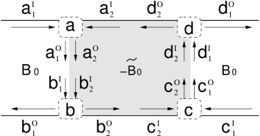
Figure 6: The same as Fig. 5(a) but with detailed labeling of edge channels (represented by solid arrows) at its four scattering points $p\in\{a,b,c,d\}$ (dashed boxes). At each point $p$, there are two incoming channels with amplitude $(p_{1}^{\rm I},p_{2}^{\rm I})$ and two outgoing ones with $(p_{1}^{\rm O},p_{2}^{\rm O})$.

The interferometry is in the integer quantum Hall regime so that its electron transport can be described by edge channels, such as the edge states along ribbon edges and the magnetic edge states along the boundaries $\bar{ab}$ and $\bar{cd}$. The scattering between the edge channels occurs at four scattering points $p\in\{a,b,c,d\}$. Each point $p$ has two incoming channels with amplitude $(p_{1}^{\rm I},p_{2}^{\rm I})$ and two outgoing ones with $(p_{1}^{\rm O},p_{2}^{\rm O})$; for example, the two incoming channels to the point $a$ are one right-going and the other left-going channels along the upper ribbon edge, while the two outgoing channels from $a$ are the two magnetic edge channels along the line $\bar{ab}$ (see Fig. 6). At each point $p$, we introduce a scattering matrix $S_{p}$ which links the amplitudes of the incoming and outgoing states,

$$\left(\begin{array}[]{c}p^{\rm O}_{1}\\ p^{\rm O}_{2}\\ \end{array}\right)=S_{p}\left(\begin{array}[]{c}p^{\rm I}_{1}\\ p^{\rm I}_{2}\\ \end{array}\right)=\left(\begin{array}[]{cc}s^{p}_{11}&s^{p}_{12}\\ s^{p}_{21}&s^{p}_{22}\\ \end{array}\right)\left(\begin{array}[]{c}p^{\rm I}_{1}\\ p^{\rm I}_{2}\\ \end{array}\right).$$ (18)

The scattering matrix $S_{p}$ has a general form of $2\times 2$ unitary matrix,

$$\left(\begin{array}[]{cc}s^{p}_{11}&s^{p}_{12}\\ s^{p}_{21}&s^{p}_{22}\\ \end{array}\right)=e^{i\theta_{p}}\left(\begin{array}[]{cc}i\sqrt{1-t^{2}_{p}}e^{i\phi_{p}}&t_{p}e^{i\phi^{\prime}_{p}}\\ t_{p}e^{-i\phi^{\prime}_{p}}&i\sqrt{1-t^{2}_{p}}e^{-i\phi_{p}}\\ \end{array}\right).$$ (19)

On the other hand, while edge channels propagate from one scattering point $p$ to its neighboring point $p^{\prime}$, they acquire phase accumulation $\varphi_{pp^{\prime}}$. As a result, one has

$$(b_{1}^{\rm I},b_{2}^{\rm I}) = e^{i\varphi_{ba}}(a_{1}^{\rm O},a_{2}^{\rm O}),$$ (20)

$$(d_{1}^{\rm I},d_{2}^{\rm I}) = e^{i\varphi_{dc}}(c_{1}^{\rm O},c_{2}^{\rm O}),$$ (21)

$$c^{\rm I}_{2} = e^{i\varphi_{cb}}b^{\rm O}_{2},$$ (22)

$$a^{\rm I}_{2} = e^{i\varphi_{ad}}d^{\rm O}_{2}.$$ (23)

By combining the relations (18)-(23) and by putting $a_{1}^{\rm I}=1$ and $c_{1}^{\rm I}=0$, one can obtain the transmission probability $T=|d_{1}^{\rm O}|^{2}$ of the edge state incoming from the source (the left of the inteferometry) to the drain (the right),

$$T=\left|\frac{(t_{b}r_{a}+t_{a}r_{b}e^{-i\alpha})(t_{c}r_{d}+t_{d}r_{c}e^{-i\beta})}{1-e^{i\varphi}(t_{a}t_{b}-r_{a}r_{b}e^{-i\alpha})(t_{c}t_{d}-r_{c}r_{d}e^{-i\beta})}\right|^{2},$$ (24)

where $r_{p}=\sqrt{1-t_{p}^{2}}$, $\varphi$ contains the Aharonov-Bohm phase as well as the dynamical phase accumulated along one circulation of the closed loop $abcd$,

$$\varphi = \varphi_{ba}+\varphi_{cb}+\varphi_{dc}+\varphi_{ad}+\phi^{\prime}_{a}-\phi^{\prime}_{b}+\phi^{\prime}_{c}-\phi^{\prime}_{d}$$ (25)

$$+ \sum_{p\in\{a,b,c,d\}}\theta_{p},$$

$\alpha=\phi_{a}+\phi_{b}+\phi^{\prime}_{a}-\phi^{\prime}_{b}$, and $\beta=\phi_{c}+\phi_{d}+\phi^{\prime}_{c}-\phi^{\prime}_{d}$. The transmission $T$ can describe the Aharonov-Bohm oscillation of the Dirac fermions in the setup of Fig. 5(a), as a function of $\tilde{B}$. Note that in general the scattering matrix $S_{p}$ contains the information of the scattering between the $K$ and $K^{\prime}$ valleys.two

We close this appendix by analyzing Eq. (24) for a simple case of $t_{a}=t_{b}=t_{c}=t_{d}=t=1/\sqrt{2}$. In this case, the transmission probability can be simplified as

$$T=\frac{\cos^{2}\frac{\alpha}{2}\cos^{2}\frac{\beta}{2}}{1+2\sin\frac{\alpha}{2}\sin\frac{\beta}{2}\cos(\varphi-\frac{\alpha}{2}-\frac{\beta}{2})+\sin^{2}\frac{\alpha}{2}\sin^{2}\frac{\beta}{2}}.$$ (26)

This result shows a usual form for the Aharonov-Bohm interference, except for the factors $\cos\alpha/2\cos\beta/2$ and $\sin\alpha/2\sin\beta/2$. From the factors, one can see that there appears no interference whenever $\alpha=\pi$ or $\beta=\pi$. It happens when destructive interference occurs during the propagation from one ribbon edge to the other through the two magnetic edge channels along $\bar{ab}$ or $\bar{cd}$ in such special cases.

References

- (1) G. W. Semenoff, Phys. Rev. Lett. 53, 2449 (1984).
- (2) F. D. M. Haldane, Phys. Rev. Lett. 61, 2015 (1988).
- (3) K. S. Novoselov, A. K. Geim, S. V. Morozov, M. I. Katsnelson, I. V. Grigorieva, S. V. Dubonos, and A. A. Firsov, Nature 438, 197 (2005).
- (4) Y. Zhang, Y. W. Tan, H. L. Stormer, and P. Kim, Nature 438, 201 (2005).
- (5) See, e.g., T. Chakraborty and P. Pietiläinen, The Quantum Hall Effects: Integral and Fractional (Springer, 1995).
- (6) C. Berger, Z. Song, X. Li, X. Wu, N. Brown, C. Naud, D. Mayou, T. Li, J. Hass, A. N. Marchenkov, E. H. Conrad, P. N. First, and W. A. de Heer, Science 312, 1191 (2006).
- (7) F. Miao, S. Wijeratne, Y. Zhang, U. C. Coskun, W. Bao, and C. N. Lau, Science 317, 1530 (2007).
- (8) R. G. Mints, JETP Lett. 9, 387 (1969).
- (9) J. E. Müller, Phys. Rev. Lett. 68, 385 (1992).
- (10) H.-S. Sim, K.-H. Ahn, K. J. Chang, G. Ihm, N. Kim, and S. J. Lee, Phys. Rev. Lett. 80, 1501 (1998).
- (11) B. I Halperin, Phys. Rev. B 25, 2185 (1982).
- (12) A. Nogaret, S. J. Bending, and M. Henini, Phys. Rev. Lett. 84 2231 (2000).
- (13) F. M. Peeters and A. Matulis, Phys. Rev. B 48, 15166 (1993).
- (14) S. M. Badalyan and F. M. Peeters, Phys. Rev. B 64, 155303 (2001).
- (15) J. Reijniers, A. Matulis, K. Chang, F. M. Peeters, and P. Vasilopoulos, Europhys. Lett. 59, 749 (2002).
- (16) J. Reijniers, F. M. Peeters, and A. Matulis, Phys. Rev. B 59, 2817 (1999).
- (17) K. S. Novoselov, A. K. Geim, S. V. Dubonos, Y. G. Cornelissens, F. M. Peeters, and J. C. Maan, Phys. Rev. B 65, 233312 (2002).
- (18) N. Kim, G. Ihm, H.-S. Sim, and K. J. Chang, Phys. Rev. B 60 8767 (1999).
- (19) H. A. Carmona, A. K. Geim, A. Nogaret, P. C. Main, T. J. Foster, M. Henini, S. P. Beaumont, and M. G. Blamire, Phys. Rev. Lett. 74, 3009 (1995).
- (20) P. D. Ye, D. Weiss, R. R. Gerhardts, M. Seeger, K. von Klitzing, K. Eberl, and H. Nickel, Phys. Rev. Lett. 74, 3013 (1995).
- (21) I. S. Ibrahim and F. M. Peeters, Phys. Rev. B 52, 17321 (1995).
- (22) A. Matulis, F. M. Peeters, and P. Vasilopoulos, Phys. Rev. Lett. 72, 1518 (1994).
- (23) H.-S. Sim, G. Ihm, N. Kim, and K. J. Chang, Phys. Rev. Lett. 87, 146601 (2001).
- (24) A nonuniform magnetic field has been generated by applying a uniform field to a nonplanar 2D system. See, e.g., M. L. Leadbeater, C. L. Foden, J. H. Burroughes, M. Pepper, T. M. Burke, L. L. Wang, M. P. Grimshaw, and D. A. Ritchie, Phys. Rev. B 52, R8629 (1995).
- (25) A. De Martino, L. Dell’Anna, and R. Egger, Phys. Rev. Lett. 98, 066802 (2007).
- (26) N. N. Lebedev, Special Functions and Their Applications (Dover Publications, Inc., NewYork, 1972).
- (27) In the presence of the step potential, depends on the eigenenergy of the Dirac Hamiltonian in Eq. (4); for example, one finds for . As a result, should be studied in a self-consistent way [see Eq. (7)].
- (28) L. Brey and H. A. Fertig, Phys. Rev. B 73, 195408 (2006).
- (29) See, e.g., R. Saito, G. Dresselhaus, and M. S. Dresselhaus, Physical Properties of Carbon Nanotubes (Imperial College Press, 1998).
- (30) Y. Meir and N. S. Wingreen, Phys. Rev. Lett. 68, 2512 (1992).
- (31) S. Datta, Electronic Transport in Mesoscopic Systems (Cambridge University Press, Cambridge, UK, 1995).
- (32) H.-S. Sim, C.-J. Park, and K. J. Chang, Phys. Rev. B 63, 073402 (2001).
- (33) D. A. Abanin, P. A. Lee, and L. S. Levitov, Phys. Rev. Lett. 96, 176803 (2006).
- (34) L. Oriszlány, P. Rakyta, A. Kormányos, C. J. Lambert, and J. Cserti, Phys. Rev. B 77, 081403(R) (2008).
- (35) T. K. Ghosh, A. De Martino, W. Häusler, L. Dell’Anna, and R. Egger, Phys. Rev. B 77, 081403(R) (2008).
- (36) The scattering between the valleys and has been studied in a graphene ribbon. See, e.g., J. Tworzydlo, I. Snyman, A. R. Akhmerov, and C. W. J. Beenakker, Phys. Rev. B 76, 035411 (2007).