Ergodicity and Slowing Down in Glass-Forming Systems with Soft Potentials: No Finite-Temperature Singularities

Abstract

The aim of this paper is to discuss some basic notions regarding generic glass forming systems composed of particles interacting via soft potentials. Excluding explicitly hard-core interaction we discuss the so called ‘glass transition’ in which super-cooled amorphous state is formed, accompanied with a spectacular slowing down of relaxation to equilibrium, when the temperature is changed over a relatively small interval. Using the classical example of a 50-50 binary liquid of $N$ particles with different interaction length-scales we show that (i) the system remains ergodic at all temperatures. (ii) the number of topologically distinct configurations can be computed, is temperature independent, and is exponential in $N$. (iii) Any two configurations in phase space can be connected using elementary moves whose number is polynomially bounded in $N$, showing that the graph of configurations has the ‘small world’ property. (iv) The entropy of the system can be estimated at any temperature (or energy), and there is no Kauzmann crisis at any positive temperature. (v) The mechanism for the super-Arrhenius temperature dependence of the relaxation time is explained, connecting it to an entropic squeeze at the glass transition. (vi) There is no Vogel-Fulcher crisis at any finite temperature $T>0$.

I Introduction

It is not uncommon to read in papers devoted to the glass-transition a statement of the type ‘it is well known that glass forming systems lose ergodicity’. It is even more common 96EAN to use fits of the $\alpha$ relaxation-time $\tau_{\alpha}$ in such systems to the Tamam-Vogel-Fulcher formula

$$\tau_{\alpha}\propto\exp\bigl{(}AT/(T-T_{\rm VF})\bigr{)}\ ,$$ (1)

which indicates a belief that the relaxation time actually diverges at some temperature $T_{\rm VF}>0$. Related to these issues is the concept of the Kauzmann temperature 48Kau which is a finite temperature $T_{\rm K}>0$ where the extrapolated entropy appears to vanish. In this paper we argue that these related questions should be addressed with care; we wish to clarify which of these issues can actually appear in glass-forming systems, and which of them are only a consequence of inadequate simulations or interpretations, or even of a confusion of questions.

In some parts this paper is a review, or an outgrowth of our own efforts to understand basic concepts of glass-formation, which became more transparent in some of our earlier work 07ABHIMPS ; 07HIMPS ; 07Eck , and whose findings we combine in this paper. Glasses and their formation have occupied researchers for many decades, with ideas being first developed on theoretical bases 01Don , and, in more recent years, being studied extensively with the help of computer simulations 89DAY ; 99PH ; 04DA ; 06ST . Such simulations vary from very realistic models to toy models with simplified dynamics, but correspondingly faster simulations. We can summarize our findings in the following logical structure:

1) One has to distinguish between large (but finite) systems as compared to infinite systems. Infinite systems pose difficult conceptual problems, because in this case, density and close packing are not tightly related (any small lowering of density will allow for arbitrarily large voids, and the jamming problems disappear).

We will therefore focus our discussion only on systems with a finite, but arbitrary, number of particles. In this view an Avogadro number of particles is finite, and it is important to state this fact.

2) There is an essential difference between systems or particles with a hard core and systems of particles interacting with soft repulsive potentials. In the first case, there is obviously a density where the particles can not move any more (or at least not all of them can be moved). This poses interesting problems of jamming, or contact geometry. These issues have been studied in depth by Stillinger and his school, with a careful analysis of different types of ‘movability’ 06Don . We point out that these problems, while very interesting from the geometrical point of view (see also the book by Conway and Sloane Con ) do not really address the questions of what a generic glass is. We will thus focus attention to systems with a finite number of particles, and with soft potentials.

3) There is another issue which deserves attention: time. Many concepts of glasses are based on the notion that if something does not happen before a given time, then it will never happen. Such reasoning is unacceptable from a theoretical point of view, since a natural time scale does not exist. We will argue that in systems with a finite number of particles interacting via soft potentials there is no singularity in the relaxation time at any positive temperature. In particular such systems undergo a glass ‘transition’ in the sense that their relaxation time increases without limit as temperatures are lowered, but they remain ergodic. Observing the consequences of ergodicity may necessitate waiting for an unbounded, but still finite time. At any temperature larger than $T=0$ all of phase space is available to the system, all the configurations are dynamically connected; the configurational entropy can be computed, yielding a finite result for any given finite energy (or finite temperature). We stress and reiterate that this paper deals with systems having a finite number of particles, which are interacting via soft potentials and are being observed for an unbounded time.

One can exemplify the discussion with the help of many simple models, and for concreteness we choose the classical example of a glass forming binary mixture of particles interacting via a soft $1/r^{12}$ repulsion with a ‘diameter’ ratio of 1.4. More or less related models can be found in FA1984 ; davisonsherrington2000 ; sh2002 ; schliecker2002 ; Jstatmech2007 ; benarous2006 . This 2-dimensional model had been selected for simulation speed and, more importantly, for the ease of interpretation. We refer the reader to the extensive work done on this system 89DAY ; 99PH ; 07ABHIMPS ; 07HIMPS ; 07IMPS . It shows that it is a bona fide glass-forming liquid meeting all the criteria of a glass transition. In short, the system consists of an equimolar mixture of two types of particles with diameter $\sigma_{2}=1.4$ and $\sigma_{1}=1$, respectively, but with the same mass $m$. The three pairwise additive interactions are given by the purely repulsive soft-core potentials

$$u_{ab}=\epsilon\left(\frac{\sigma_{ab}}{r}\right)^{12}\ ,\quad a,b=1,2\ ,$$ (2)

where $\sigma_{aa}=\sigma_{a}$ and $\sigma_{ab}=(\sigma_{a}+\sigma_{b})/2$. The cutoff radii of the interaction are set at $4.5\sigma_{ab}$. The units of mass, length, time and temperature are $m$, $\sigma_{1}$, $\tau=\sigma_{1}\sqrt{m/\epsilon}$ and $T=\epsilon/k_{B}$, respectively, with $k_{B}$ being Boltzmann’s constant.

It has been shown that for temperatures $T>0.5$ the system behaves like a liquid. For temperatures lower than 0.5 the system begins to slow down, the correlation functions stop decaying exponentially, and can be fitted within reason to a stretched exponential form, cf. Fig. 1.

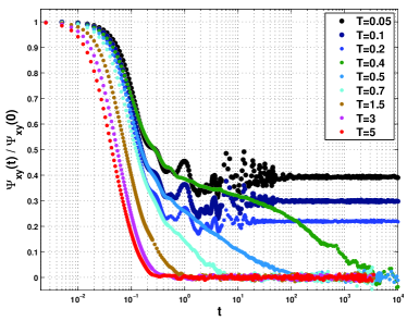
Figure 1: (Color online:). Typical correlation functions at different temperatures for the model under discussion. Shown are the shear stress-shear stress correlation function which decays exponentially at high temperatures, and then, at about $T=0.5$, changes character to a stretched exponential form. At temperatures lower than 0.4 the correlations decay to a finite value, which is determined by the mean shear modulus, indicating that the material behaves like a solid for the given measurement time. For further details about these measurements see 08IPS .

The time constant (or so-called $\alpha$ relaxation time) can be fitted to the Vogel-Fulcher form (1) for temperatures not too close to $T_{\rm VF}$. The model shows the expected behavior of the specific heat at the temperature range that is considered the ‘glass transition’ (i.e., where the relaxation time increases rapidly), and the ‘super-Arrhenius’ dependence of the viscosity on the temperature. In short, the system appears as a good example to consider to elucidate the fundamental issues that concern us here.

In Sect. II we explain how to discretize the configurational space using Voronoi tesselations and their dual Delaunay triangulations. This offers the basis of the demonstration of ergodicity at any finite temperature. We also review the mathematical results concerning the size of this phase space (exponential in the number of particles $N$) and the fact that its graph has the small-world property in the sense that any configuration can be reached from any other using a polynomial number of steps. In Sect. III we discuss the configurational entropy, and explain that there is never a Kauzmann crisis in this system. Finally in Sect. IV we present the fundamental reason for the ‘super-Arrhenius’ dependence of the relaxation time on the temperature. This is due to the fast decrease in the concentration of some quasi-species, leading to an entropic squeeze. In Sect. V we summarize the paper and offer concluding remarks.

II Voronoi construction and ergodicity

II.1 Voronoi tessellation and Delaunay triangulation

We begin by discussing the possible configurations of the system in a systematic way, using the time-honored Voronoi polygon construction 89DAY . It associates with every configuration of the particles a subdivision of position space into polygons, one per particle. These polygons will also be called cages. The polygon associated with any particle contains all points closer to that particle than to any other particle. The edges of such a polygon are the perpendicular bisectors of the vectors joining the center of the particle (actually the coordinates of the point particles we consider). As had been noted in 89DAY ; 99PH , when periodic boundary conditions are used, the average number of sides of the polygons is exactly 6. This follows because the Euler characteristic on the torus is 0: $\chi=V-E+F=0$, where $V$, $E$, and $F$ are respectively the numbers of vertices (corners), edges and faces in the given polyhedron.

Typical such Voronoi tessellations for two different temperatures are shown in Fig. 2. Since there are two types of particles (small or large, or blue and red (respectively)), in order to have a mapping between the particle positions and the number of sides in the polygons of the Voronoi tessellation, we distinguish between polygons having a small and large particles in their center. Thus, a coloring scheme of cells will take into account not only the number of sides, but also the type of the particle (big or small) in each cell. The tessellation obtained without distinguishing the type of particles will be referred to as ‘colorless’ and so, below, will be the resulting triangulation. When distinguishing the two types of particles, the tessellation and its triangulation will be referred to as colored.

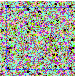
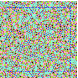
Figure 2: Upper panel: The Voronoi polygon construction in the liquid state at $T=3$ with the seven-color code used in this paper. Small particles in pentagons (heptagons) are light green (dark green) and large particles in pentagons (heptagons) are violet (pink). Lower panel: a typical Voronoi construction in the glass phase at $T=0.1$. Note the total disappearance of liquid-like defects (large particles in pentagons and small particles in heptagons).

Note that in a generic configuration the Voronoi decomposition has the property that exactly three lines meet at a point. Accordingly, the dual graph of such a decomposition is a triangulation. Such triangulations are called Delaunay triangulations. They are obtained by simply connecting the centers of those particles which are separated by one edge of the polygon. In other words, the vertices of the triangles coincide with the particles at the centers of the Voronoi cells. Let us remark that this construction can be also done in 3-dimensions (or more), where now instead of edges of polygons we have faces of polyhedra and four faces will meet at a point. In this case, the dual graphs are now made of tetrahedra. In 3-dimensions we will call the graphs obtained in this way Delaunay tetrahedrization. It is noteworthy that there is an important difference between 2 and 3-dimension. In 2-dimensions, the points of any triangulation can be arranged in such a way in position space that the triangulation is indeed a Delaunay triangulation, as described above, that is, the dual of a Voronoi decomposition. However, in 3-d there exist tetrahedrizations which are not duals of Voronoi tessellations, or in other words, cannot be obtained starting with particles spread in 3-dimensions, mapped onto a Voronoi tessellation and then tetrahedrized (06santos ).

Having outlined the description of configurations in this model (and in fact all models of this general type), we consider now the question of dynamic accessibility, viz. ergodicity. The model under consideration is Hamiltonian, but in simulations it is coupled to a heat bath of temperature $T$. There are several methods for achieving such a coupling, leading to the study of this model in either $N$, $V$, $T$ or $N$, $p$, $T$ ensembles. In either ensemble the mean energy per particle is fixed, but there can be arbitrarily large fluctuations in the energy. It is precisely these fluctuations which are the source of ergodicity. The energy is partially kinetic and partially potential. By ergodicity, one means that the natural motion of the system can reach every point in phase space. For systems having one type of (indistinguishable) particles, it is not important to look at particles exchanging positions: indeed every point in phase space can be obtained by moving particles within their cages and translating cages as is necessary. In contrast, when there is more than one type of particle (here we have two types), ergodicity means that particles must also be able to change their relative positions in all imaginable ways. It is therefore useful in both cases to distinguish between thermal motion of individual particles rattling in their own ‘cages’, without really changing their relative positions, and large scale movements and exchanges of particles that change the macroscopic configuration. Only the second class of movements is important in terms of the configurational entropy of the system, which arises from counting different configurations, for which the thermal motion does not matter. For example, in systems with hard core interactions, there are various levels at which motion can be restricted, as we have mentioned before. But here, we consider soft particles.

Since we are starting from a problem with particles which live in a concrete space, we can focus on the restricted class of Delaunay graphs (which actually coincides in 2-d with all triangulations, as we have explained earlier). In other words, in 2-dimensions (3-dimensions) the natural phase-space for our system is the set of all Delaunay triangulations (tetrahedrization).

In 2-dimensions the elementary change in the Voronoi tessellation is obtained by a so called $T_{1}$ process as seen in Fig. 3. (This operation has various names in the literature: Gross-Varstedt move, Pachner move, flip.) Malyshev1999 ; Negami1999 ; Mori2003 ; pach78 ; pach81 . Note that the operation of a $T_{1}$ process in the Voronoi tessellation translates to a flip in the Delaunay triangulation, see Fig. 3.

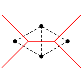
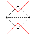
Figure 3: A T1 process in the Voronoi tessellation (in red lines) and the equivalent flip process in the Delaunay triangulation (dashed curves)

To simplify things further, we consider instead of the triangulations of the torus the triangulations ${\cal T}$ of the sphere. The simplification is that the genus is 0, and that more is known about the combinatorics of triangulations of the sphere than of the torus. Given $N$, corresponding to the number of particles in the original model, we let ${\cal T}$ denote a triangulation of the sphere with $N$ nodes and we let ${\mathbb{T}}_{N,0}$ denote the set of all such triangulations. By this, one means the set of all combinatorially distinct rooted simplicial 3-polytopes. In particular, a triangulation should not have any ‘double edges’. We further refine the definition, by distinguishing 2 types of nodes in the triangulation: We first number the nodes from 1 to $N$ and then define 2 types of nodes. Those with even index are the ‘small particles’ and those with odd index the ‘large’ ones. This means that the triangulation has the same number of large and small nodes (up to a difference of one). We will also call the two types of nodes two colors.

We shall call the odd nodes blue and the even ones red and will refer to the triangulations as colored triangulations. Once the colors are assigned, the numbers are again forgotten. The set of all colored triangulations with $N$ nodes will be called ${\mathbb{T}}_{N}$. This is our phase space and the dynamics is mapping points in this phase space to other points. Having understood that, we can now ask the major question of this section:

The question of ergodicity: is every point in phase-space accessible through a sequence of motions that are flips. The answer is not obvious from the outset. For example in 2-dimensions one can consider a triangulation that includes locally a form as in Fig. 4.

Figure 4: A configuration with four nodes that cannot be flipped, because that would lead to double links. In 3-dimensions there is more than one corresponding graph, but none of them is the dual of a Voronoi 06santos ,

Obviously, a form like this is stuck, since one cannot do any flip without doubling one of the links. (One can see this easily by noticing that the configuration in Fig. 4 is a valid triangulation of the sphere, and it is the unique triangulation with four points.) The question of ergodicity is even less trivial in 3-dimension, where there is a whole class of unflippable tetrahedrizations. However, they are not duals of Voronois. But, the relevant question (in any dimension) is whether the triangulations (tetrahedrizations,…) which are duals of Voronoi tessellations are indeed all connected in one large component. The answer is nevertheless ‘yes’ in both 2 and 3-dimensions as we explain next.

II.2 Demonstration of ergodicity

One can attack this problem in two ways, the first being more physical, and the second more mathematical. The physical argument is trivial. Since the particles are soft, and the energy is not bounded, they can be moved around each other in any way one can imagine. We stress again that while this needs perhaps a lot of energy, the large fluctuations of the energy will guarantee that this will eventually happen, rarely, but surely. And hence ergodicity is obvious. The only care one must observe is that moves through degenerate situations (4 lines meeting at a Voronoi vertex) must be avoided.

The question is more intriguing when formulated in terms of triangulations alone, since we have seen in Fig. 4 that a local configuration in which 3 links emanate from a node cannot be flipped. Could it be that the triangulation is so imbricated that in fact none of the edges can be flipped? Indeed, for 4 particles this is exactly what happens, but then, the phase space consists of exactly one triangulation and thus there is no need to move any link. In 1936, Wagner Wagner1936 showed that a finite number of flips will transform any triangulation of the sphere into a ‘Christmas tree,’ which is the configuration shown in Fig. 5. See also CE2005 for a discussion of several related issues.

Figure 5: The Christmas tree. Two nodes are at the bottom, the others (only 4 shown) are in the stem of the tree.

Since one can undo the flips, this implies immediately that any two triangulations can be connected by a sequence of flips going through the christmas tree. There is abundant literature on this question 06santos ; Negami1999 which also plays a certain role in the classification of 3-manifolds.

II.3 The size of phase space

The possible states of our system of triangulations with $N$ nodes is the set ${\mathbb{T}}_{N}$ of all possible colored triangulations. The set ${\mathbb{T}}_{N}$ has, as we will see, a number of elements which grows like $C^{N}$ for some constant $C>1$. It is thus a discrete space with a finite number of states. To describe the dynamics of flipping in a geometric way, one should view this set as the dynamical graph $\cal G$, whose nodes are now the elements of the set ${\mathbb{T}}_{N}$ (not to be confused with the nodes (particles) of any triangulation ${\cal T}$) and two of its nodes are linked if one can be reached from the other by a flip. (This makes an undirected graph, since one can flip back and forth.) The reader should note that there are two graphs in this discussion: Each triangulation is a graph with $N$ nodes, and $3N-6$ links (by Euler’s theorem), while the graph $\cal G$ has about $C^{N}$ nodes, and about $3N-6$ links per node. This last statement follows because in every state of ${\mathbb{T}}_{N}$, one can choose which of the $3N-6$ links of the triangulation ${\cal T}$ one wants to flip. However, there will, in general, be somewhat fewer links which are candidates for flipping, because whenever there is a node of degree $3$ in the triangulation ${\cal T}$ its links can not be flipped (a tetrahedron is unflippable).

Finally, given any two elements in ${\mathbb{T}}_{N}$, that is, any two triangulations with $N$ nodes, we will show below that ${\cal O}(N^{2})$ flips are sufficient to walk on the graph $\cal G$ from one to the other. Thus, the diameter of the graph $\cal G$ is at most ${\cal O}(N^{2})$ while it has ${\cal O}(1)^{N}$ vertices. This means that $\cal G$ has the ‘small-world’ property Watts1998 . It has also small clustering coefficient, since there are very few triangles in the graph $\cal G$ (it is difficult to get from a triangulation back to the same triangulation with 3 flips).

In the remainder of this section, we spell out these statements. They are well-known for uncolored graphs, so the only task is to prove them for the colored graphs, see 07Eck .

We first state two known results for the set ${\mathbb{T}}_{N,0}$ of uncolored triangulations:
Lemma 1 Tutte1962 ; Negami1999 ; Mori2003 The number of elements in ${\mathbb{T}}_{N,0}$ is asymptotically

$$\left(\frac{256}{27}\right)^{N-3}\frac{3}{16\sqrt{6\pi N^{7}}}~{}.$$ (3)

The distance between any two uncolored triangulations is at most $6N-30$ flips.

For the case of the colored graphs, with $N_{\rm red}=N_{\rm blue}+c$ and $c\in\{0,1\}$, that is, about equal number of red and blue nodes, one has
Lemma 2 The number of elements in ${\mathbb{T}}_{N}$ is asymptotically bounded above by

$$2^{N}\left(\frac{256}{27}\right)^{N-3}\frac{3}{16\sqrt{6\pi N^{5}}}~{},$$ (4)

and below by the expression (3). The distance between any two colored triangulations in ${\mathbb{T}}_{N}$ is bounded by

$$C_{1}N^{2}+C_{2}$$ (5)

flips with some universal constants $C_{1}$, $C_{2}$.

We note that the phase space as defined here is (obviously) independent of the temperature. We can thus conclude that the present classical model of glass-formation does not suffer from any issue of loss of ergodicity. Accordingly, it should have a valid statistical mechanics at any temperature $T>0$. Next we show that indeed its configurational entropy $S$ never suffers any finite temperature crisis, and there is no Kauzmann temperature where $S\to 0$

III Configurational Entropy

III.1 Statistical Mechanics

Needless to say, the configurations discussed in the previous section have different energies and therefore the probability to see any particular one can be strongly dependent on the temperature. To discuss the temperature dependence of the configurational entropy of this system we need to review the statistical mechanics that was introduced for this system in 07HIMPS . The basis of the analysis is again the Voronoi tessellation.

To get some systematics, we first define a ‘typical’ energy for each type of topological cell, with an average taken over all cells with a given number of sides and a given particle type (big or small) in its center. The average is then $\epsilon_{i}=\langle\,\sum_{k=1}^{E_{i}}\epsilon\left(\frac{\sigma_{ik}}{r_{ik}}\right)^{12}\rangle$ where $E_{i}$ is the number of edges associated with that cell type ($i$), and $r_{ik}$ being the distance to the particle in the adjacent Voronoi cell and the average is over all particles of the same type $i$. In Fig. 6 we present the values of these energies measured numerically as a function of the temperature, following a protocol of slow cooling. In the range of temperatures explored by simulations there are 10 different cell types, (large particle or small particle in squares, pentagons, hexagons, heptagons and octagons), but octagons and squares are not shown since they already disappear at relatively high temperature, much above the glass transition.

We learn from these data graphs that the different cell types have clearly split energies throughout the interesting temperature range, and that these energies are only weakly dependent on the temperature. Within the temperature range of interest we can focus on the six types of cells; denote by $\{N_{i}\}_{i=1}^{6}$ the number of cells of each type, with number of edges $E_{i}$, ordering them by the mean energy $\epsilon_{i}$ with $i=1$ being the highest (large particle in a pentagon) and $i=6$ being the lowest (small particle in an heptagon). Additional important properties of the cell types are their areas $\Omega_{i}$ and their shapes; the first affects the enthalpy term and both affect the configurational entropy when we count the number of possible tilings of the plane.

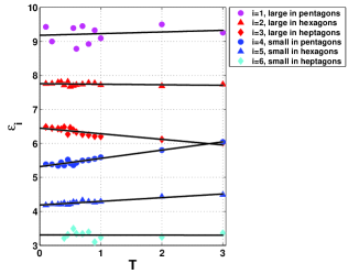
Figure 6: (Color online). The average energies of the Voronoi cells as a function of the temperature as measured in the simulations.

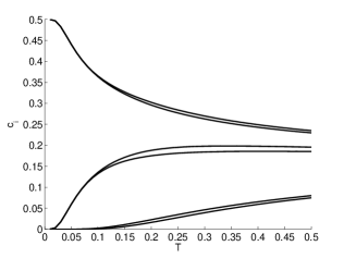
Figure 7: The concentrations of all the Voronoi cells as a function of $T$. Note the close-to-degeneracy of pairs of cells: the upper pair are the glass-like quasi-species, the middle pair are the two hexagons and the lower pair the liquid-like quasi-species. Observe the existence of two typical temperatures ranges, one around $T_{2}$ where the liquid-like quasi-species deplete severely, and the other around $T_{1}$ where the hexagons deplete rapidly.

With this in mind we can construct the statistical mechanics of this system by considering the free energy $G=U+pV-TS$. We should stress at this point that one could aspire for more accurate statistical mechanics, considering for example not only the type of particle inside the Voronoi n-gon, but also who are the neighbors (small or large particles) (which resembles somehow the plaquette expansions in statistical mechanics). Such a choice would have allowed a better treatment of the tendency of hexagons with large (or small) particles for example to crowd together to minimize the $pV$ term in the free energy. The price is that the number of quasi-species increases to 42 (6, 7 and 8 for each pentagon, hexagon and heptagon respectively). While doable and a bit more precise, this more involved statistical mechanics does not shed more light on the issues of principle that interest us in the present paper, and therefore we do not discuss such improvements any further.

Coming back to the simpler variant, we note that in the free energy the value of $U$ is $\sum_{i=1}^{6}N_{i}\epsilon_{i}$. The $pV$ term is simply $p\sum_{i=1}^{6}N_{i}\Omega_{i}$. Lastly, we need to estimate the entropy term. In principle this should be computed from the number of possible complete tilings of the area by $N_{i}$ cells of each type with its given area and shape, subject to the Euler constraint $\sum_{i=1}^{6}N_{i}E_{i}=6N$, where $E_{i}$ is the number of edges of the $i$’th polygon. This is a formidable problem. A useful estimate can be obtained by considering the area only, and filling space starting with the largest objects, then the next largest, and so on, until the smallest are fit in. We do this by dividing the (remaining) volumes into boxes, and studying the combinatorial filling of these boxes. Denoting the possible number of boxes to fit the largest cells by ${\cal N}_{1}\equiv V/\Omega_{1}$, then the number of boxes available for the second largest cell by ${\mathcal{N}}_{2}\equiv(V-N_{1}\Omega_{1})/\Omega_{2}$ etc., the number of possible configurations $W$ is

$$W=\prod_{i=1}^{6}\frac{{\mathcal{N}}_{i}!}{N_{i}!({\mathcal{N}}_{i}-N_{i})!}\ .$$ (6)

Using the abbreviation $x_{i}\equiv N_{i}/{\mathcal{N}}_{i}$ we compute directly $x_{i}=c_{i}\Omega_{i}/\sum_{j=i}^{6}c_{j}\Omega_{j}$ where $c_{i}$ is the number concentration of each defect. We can now compute $S=k_{\rm B}\ln W$ and write $G$ together with a Lagrange multiplier for the Euler constraint,

$$G=\sum_{i=1}^{6}N_{i}\epsilon_{i}+p\sum_{i=1}^{6}N_{i}\Omega_{i}+\lambda\sum_{i=1}^{6}N_{i}E_{i}$$

$$+T\sum_{k=1}^{6}{\mathcal{N}}_{k}[x_{k}\ln x_{k}+(1-x_{k})\ln(1-x_{k})]\ .$$ (7)

The chemical potential $\mu_{i}\equiv\partial G/\partial N_{i}$ is then, for $i=1,\dots,6$,

$$\mu_{i}=\epsilon_{i}+p\Omega_{i}+T[\ln x_{i}+\sum_{k=1}^{i-1}\frac{\Omega_{i}}{\Omega_{k}}\ln(1-x_{k})]+\lambda E_{i}\ .$$ (8)

We now recognize that Voronoi cells of different values $E_{i}$ but with the same size particle (small or large) are in equilibrium, each one being able to change to another, but small particles cannot change to large particles, and therefore in equilibrium there exist only two independent values of $\mu_{i}$, one for the small particles $\mu_{S}$ and one for the large particles $\mu_{L}$, and we have 9 unknowns – six values of $c_{i}$, 2 values of $\mu$ and one Lagrange multiplier $\lambda$. This is precisely balanced by the 6 equations (8), the Euler constraint, and the two constraints $\sum_{i=1}^{3}c_{i}=\sum_{k=4}^{6}c_{k}=1/2$. These equations could be solved numerically using the precise values of $\Omega_{i}(T)$ and $\epsilon_{i}(T)$ as measured in the simulation. The approximate calculation of the entropy however does not warrant such a detailed calculation. In reality, calculating the average areas of the cell types in the numerical simulations, we discover that to an excellent approximation these fall in two classes, smaller cells of area $\Omega_{S}$ when small particles are in them, and larger cells of area $\Omega_{L}$ where large particles are enclosed. These areas again are only weakly dependent on the temperature. Then the whole system of equations simplifies to two analytically tractable sets of equations

$$\tilde{\mu}_{L} = \epsilon_{i}+T\ln c_{i}+\lambda E_{i}\ ,\quad\{i=1,2,3\}\ ,$$

$$\tilde{\mu}_{S} = \epsilon_{i}+T\ln c_{i}+\lambda E_{i}\ ,\quad\{i=4,5,6\}\ ,$$ (9)

together with the above mentioned three constraints. In $\tilde{\mu}$ we have absorbed terms that added to $\mu$ in this special case.

In Fig. 7 we show the solutions of these equations when we use values of $\epsilon_{i}$ taken from the Fig. 6 at $T=0$. We learn from these results that the statistical mechanics predicts that the first quasi-species to disappear are the large particles in pentagons and the small particles in heptagons. While the first is the highest in energy, the disappearance in tandem of the second is a result of the Euler constraint, and could not be guessed a priori. In previous work the first disappearing quasi-species were called ‘liquid-like’, since they are common in the liquid state and their concentration is exponentially small in the glass state. The region of temperature where their concentration falls off rapidly was identified with the region of slowing down. In fact, in 07HIMPS a quantitative relation between the concentration of these liquid-like quasi-species and the relaxation time was derived, explaining the slowing down as a result of an entropic squeeze. We will return to this issue in Sect. IV.

The statistical mechanics predicts a second transition (cf. Fig. 7). Below some temperature the concentration of hexagonal cells is predicted to be exponentially small, and the system retains only pentagons with small particles and heptagons with large particles. These are referred to as the ‘glass-like’ quasi-species. Indeed, in 07HIMPS it was found that a phase made of only pentagons with small particles and heptagons with large particles exists and is stable at low temperatures, see Fig. 8.

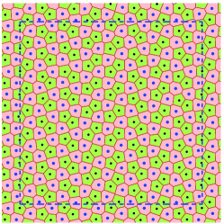
Figure 8: (Color online). An example of a stable phase formed by glass-like quasi-species at very low temperatures.

Upon warming up such a phase, at a temperature roughly around $T_{1}$, a sizable number of hexagons appears to form the generic glassy state. Upon further warming, crossing a temperature roughly around $T_{2}$, a sizable number of liquid-like defects brings the system to a liquid state. The actual values of $T_{1}$ and $T_{2}$ can be understood from this model. Denote by $c_{\ell}$, $c_{H}$ and $c_{G}$ the concentrations of the liquid-like, hexagons and glass-like quasi-species, and by $\epsilon_{\ell}=\epsilon_{1}+\epsilon_{6}\approx 12.48$ as the energy associated with the liquid-like quasi-species, by $\epsilon_{H}=\epsilon_{2}+\epsilon_{5}\approx 11.94$ the energy of the hexagons, and $\epsilon_{G}=\epsilon_{3}+\epsilon_{4}\approx 11.76$ the energy of the glass-like defects. The theory predicts that ratios $c_{\ell}/c_{H}$ and $c_{H}/c_{G}$ are of the order of $\exp[-(\epsilon_{\ell}-\epsilon_{H})/T]$ and $\exp[-(\epsilon_{H}-\epsilon_{G})/T]$ respectively. As an estimate of $T_{2}$ and $T_{1}$ take these ratios to be, say, of the order of $1\%\sim\exp(-5)$ and observe that such ratios are obtained for $T=T_{2}\approx 0.11$ and $T=T_{1}\approx 0.04$. It is important to notice that $\epsilon_{H}-\epsilon_{G}$ could be positive rather than negative, and then the system would crystallize on a hexagonal lattice. Such a lattice can exist in this system only when the particles phase separate into two pure hexagonal lattices of small and large particles respectively, with an interface in between. Such a phase may even be the ground state, but seems to be inaccessible in dynamical experiments starting from random organizations of small and large particles.

III.2 Nonexistence of Kauzmann temperature

Assuming that indeed the realized state at $T=0$ is the state shown in Fig. 8, but equivalently if the ground state were made of hexagons, it is obvious now that any finite temperature will allow the appearance of the other quasi-species (hexagons inside the phase in Fig. 8 or pairs of pentagons and heptagons in the hexagonal phase if the latter were the ground state). Focusing on the first situation, we understand that any pair of hexagons costs a given amount of energy $\epsilon_{H}$ which is a given $\Delta$ above the ground-state $\epsilon_{G}$. The calculation given by Eq. (7) is legitimate at any temperature $T$, and the configuration entropy is approximately correct as stated there. One can improve the calculation of the entropy compared to the approximation employed above, but there is nothing extraordinary that is expected at any temperature. We thus state that the configurational entropy is expected to be an analytic function of $T$ at any value of the temperature, and it can vanish only at $T=0$. There is no Kauzmann temperature here or in any similar generic model.

III.3 The notion of fictive temperature

Notwithstanding all of the above, the system under study can slow down so much that upon reducing the temperature one has to wait for a very long time before equilibrium is reached. When the relaxation times are already very large, say at an initial temperature $T_{\rm i}$, any rapid decrease in the temperature of the heat bath to a final temperature $T_{\rm f}$ may result in a very lethargic response of the system, which may keep the concentrations of various quasi-species at values which are consistent with $T_{\rm i}$ rather than $T_{\rm f}$. It is then perfectly legitimate to introduce the notion of a fictive temperature $T_{\rm fic}\approx T_{\rm i}$, as long as one is satisfied with short observation times. For longer and longer times the system will exhibit the process of aging, and in particular $T_{\rm fic}$ will converge to $T_{\rm f}$, reaching there with certainty if given enough time.

IV Slowing down and entropic squeeze

The aim of this section is to explain the most important aspect of glass formation, i.e., the extreme slowing down in relaxation to equilibrium when the temperature is lowered. The riddle is as follows: the natural time scale is determined by the molecular jitter due to thermal motion. This time is typically of the order or $10^{-12}$s at room temperature. Glassy dynamics exhibits relaxation time $\tau_{e}$ of the order of seconds, or hours, sometimes years. How is it that such a huge gap in time scale is obtained without geometrical obstruction (as is the main theme of this paper)? We will explain that the issue is entropic squeeze, or the failure of entropy or ‘the number of available paths’ to overcome the necessary energy climb required for relaxation.

In 07ABHIMPS ; 07ILLP it was argued that the relaxation time can be predicted if one knew the typical scale $\xi$ that separates ‘liquid-like’ quasi-species. In other words, having the concentration $C_{\ell}$ of large particles in pentagons and small ones in heptagons one introduces a typical scale $\xi$ by

$$\xi\sim\frac{1}{\sqrt{C_{\ell}}}\ ,$$ (10)

since the system has two dimensions. To connect between the relaxation time $\tau_{e}$ and the length scale $\xi$ it was asserted that for the viscous fluid there exists a free energy of activation $\Delta G^{*}(T)$ associated with the relaxation event,

$$\tau_{e}=\tau_{0}\exp(\Delta G^{*}(T)/T)\ ,$$ (11)

where $\tau_{0}$ is a microscopic time scale of the order of a single particle vibration time. The free energy of activation is estimated as the number of Voronoi cells $N^{*}(T)$ involved in the relaxation event, times the (temperature independent) chemical potential per cell $\Delta\mu$, $\Delta G^{*}(T)\approx N^{*}(T)\Delta\mu$. The number $N^{*}$ depends on whether the relaxation event is a 1-dimensional 07ILLP or 2-dimensional event 07ABHIMPS . In the first case $N^{*}(T)\approx\xi(T)/\sqrt{\bar{\Omega}}$ while in the second $N^{*}(T)\approx\pi\xi^{2}(T)/4\bar{\Omega}$, where $\bar{\Omega}$ is the mean area of a Voronoi cell. We end up with the predictions

$$\tau_{e} = \tau_{0}\exp(\xi(T)\Delta\mu/\sqrt{\bar{\Omega}}T)\ ,\text{1-d event}\ ,$$ (12)

$$\tau_{e} = \tau_{0}\exp(\pi\xi^{2}(T)\Delta\mu/4\bar{\Omega}T)\ ,\text{2-d event}\ .$$ (13)

These predictions were shown to fit the simulation data very well 07ILLP ; 07ABHIMPS . Here we want to explain the fundamental origin of these formulae.

The glass transition and the associated slowing down take place in the range of temperatures around $T_{1}$ where the liquid-like quasi-species deplete rapidly. It is advantageous theoretically to focus on the range of temperatures around $T_{2}$ where the hexagons deplete quickly, cf. Fig. 9,

Figure 9: (Color online). An example of a phase obtained by simulation at low temperatures when hexagons appear in the phase of Fig. 8. Note the tendency of hexagons to clump together, a tendency that is ignored in our approximate estimate of the configurational entropy.

since then we have a smaller number of quasi-species to take into account, while the fundamental phenomenon of entropic squeeze is not very different. So think about a situation when the majority of quasi-species are pairs of glass-like pentagons and heptagons, and set up the energy scale such that these pairs have energy zero. Next consider a temperature $T$ where the equilibrium concentration $c$ of hexagons is small, $c\ll 1$. Set up the energy units such that each pair of hexagons (one with small particle and one with large particle) has an energy $\Delta=1$. Accordingly the energy of this configuration is

$$E=cN\ .$$ (14)

One the other hand, the entropy of this configuration can be estimated as the logarithm of the number of ways the hexagons can be distributed, which is

$$S\approx-Nc\ln c=Nc\ln(1/c)\ .$$ (15)

As a result we can compute

$$\frac{\partial S}{\partial E}=\frac{1}{N}\frac{\partial S}{\partial c}=-\ln c-1\approx-\ln c~{}.$$ (16)

Remembering the thermodynamic identity $\partial E/\partial S=T$ we then conclude that the concentration of hexagons satisfies the relation

$$c=\exp(-1/T)\ .$$ (17)

Accordingly we conclude that in two-dimensions the average distance $\xi$ between hexagons, which is $\xi\approx 1/\sqrt{c}$, satisfies

$$\xi\approx\exp(1/2T)\ .$$ (18)

Whenever a pair of hexagons is created, with high probability, this will be undone sometime in the future (by the inverse operation). Once they are separated in space by the distance $\xi$, we need a number of flips which is at least of the order of $\xi$, but maybe many more, in order to annihilate a pair. This is the fundamental process of relaxation at temperature $T$ which we now proceed to estimate. In other words, we estimate how many flips are typically needed in order to get rid of one pair of hexagons, and we will show that the answer is super-Arrhenius.

We first note that because the concentration $c$ is small, any random flip will create a pair of hexagons and increase the energy by unity. Only flips that eliminate a pair of hexagons (to create a heptagon and pentagon) reduce the energy by unity. We denote the probability of such a rare event by $\gamma$. It will be crucial that $\gamma$ depends on the temperature as we will explain below. Out of all the other flips, assume that a fraction $\alpha$ of flips does not change the energy (it has to involve a hexagon and one of a pentagon-heptagon pair). What is then the best way to move one hexagon a distance $\xi$ until it can annihilate its counterpart? Assume that the path takes $m$ flips where the energy increases by one unit (a typical flip), is energy neutral over $k$ flips, and then goes down in energy in $m$ steps, with the constraint

$$2m+k\geq\xi\ .$$ (19)

Of course, these events can take place in any order. Clearly, we have a competition between the number of ways to arrange such a path and the energy barrier that needs to be surmounted, i.e., we need to sum up over all $m$ and $k$ the expression

$$P(m,k)=\frac{(2m)!}{m!\,m!\,k!}(1-\alpha-\gamma)^{m}\alpha^{k}\gamma^{m}e^{-m/T}\ .$$ (20)

Note that all the factors are smaller than 1 and therefore the sum is well approximated by the largest term, which occurs for $m=\xi/2$ and $k=0$. We thus get

$$P=\sum_{2m+k\geq\xi}P(m,k)\sim[(1-\alpha-\gamma)\gamma e^{-1/T}]^{\xi/2}\ .$$ (21)

Note now that $\alpha$ is just some number smaller than 1, but more importantly, $\gamma$, which is the probability to find an energy-lowering move is proportional to the density of defects. Indeed, if any flip is done at a link in the triangulation in which neither of its ends is a defect the energy will go up. (In fact, this reasoning also shows that $\alpha$ goes to zero when the temperature goes to 0.)

Now, the density of defects is $c=\exp(-1/T)=\gamma$ so that we get finally,

$$P\sim(e^{-1/T}e^{-1/T})^{\exp(1/2T)/2}\ .$$

The time we need to wait to see the event is proportional to the inverse of this probability, or

$$\tau_{e}\propto\exp{(\xi/T)}$$ (22)

which is precisely Eq. (12). This is the one appropriate for 1-dimensional relaxation events as assumed here and the generalization to other dimensions is obtained by modifying the relation between the density and $\xi$. The non-Arrhenius nature of the relaxation time is due to the strong temperature dependence of $\xi(T)$ (cf. 07ILLP ), which in turn is due to the fast disappearance of a class of quasi-species. This reduction of the number of quasi-species is responsible for the entropy squeeze.

V Summary and Conclusions

Glass forming systems with hard cores can get jammed because of geometric constraints. In this paper we argued, on the basis of a generic example, that when the potentials are soft, the spectacular slowing down associated with the glass transition is in a sense more interesting, since it does not occur due to geometric jamming. Such system never lose their ergodicity, and any configuration can be reached from any other in a polynomial (in $N$) number of steps, even though the number of configurations is exponential in the number of particles. We demonstrated explicitly that the configurational entropy in such systems if finite at any temperature, and thus neither the Kauzmann temperature nor the Vogel-Fulcher formula can be taken seriously. Both are the result of an extrapolation which is not fundamental. Finally we addressed the question of what is the reason for slowing down, and what is the mechanism of its super-Arrhenius temperature dependence. We showed by an explicit calculation for a generic relaxation step that near the glass transition when the concentration of some quasi-species becomes very small, the entropic squeeze results in the inability of the entropic counting of paths to balance the energetic barriers, leading therefore to relaxation times that depend on the temperature much faster than expected from the Arrhenius form.

In summary, we focused on the topological properties of generic glass forming systems, to clarify some fundamental issues which are not always clear in the literature. Needless to say, much of the interest in glass forming systems, including their mechanical properties, calls for understanding further issues, including metric issues that are outside the scope of this paper. For some recent thoughts on these subjects we refer the reader to 07IMPS ; 08IPRS .

Acknowlegdments. We thank F. Santos for many helpful discussions on the issues of flips. We also thank D. Mukamel for drawing our attention to related work. The work of JPE was partially supported by the Fonds National Suisse and the Joseph Meyerhoff visiting professorship. IP is supported in part by the German-Israeli Foundation, the Israel Science Foundation and the Minerva Foundation, Munich, Germany.

References

- (1) For a balanced review in which many of the common concepts and terminology are well spelled out see M.D. Ediger, C.A. Angell and S.R. Angell, J. Phys. Chem. 100, 13200 (1996).
- (2) W. Kauzmann, Chem Rev. 43, 219 (1948)
- (3) E. Aharonov, E. Bouchbinder, H.G.E. Hentschel,V. Ilyin, N. Makedonska, I. Procaccia and N. Schupper, Europhys. Lett. 77, 56002 (2007) .
- (4) H. G. E. Hentschel, V. Ilyin, N. Makedonska, I. Procaccia and N. Schupper, Phys. Rev. E 76, 052401 (2007) .
- (5) J.-P. Eckmann, J. Stat. Phys. 129, 289–309 (2007).
- (6) see E. Donth, The Glass Transition, (Springer, Berlin, 2001) and references therein.
- (7) D. Deng, A.S. Argon and S. Yip, Philos. Trans. R. Soc. London Ser A 329, 549, 575,595, 613 (1989).
- (8) D.N. Perera and P. Harrowell, Phys. Rev. E 59, 5721 (1999) and references therein.
- (9) M. J. Demkowicz and A. S. Argon, Phys. Rev. Lett. 93, 025505 (2004).
- (10) H. Shintani and H. Tanaka, Nature Physics 2, 200 (2006).
- (11) For a particularly lucid and complete discussion of these issues see A. Donev, PhD dissertation, Princeton University, 2006, and references therein.
- (12) J. H. Conway, and N.J.A. Sloane, Sphere packings, lattices and groups. Grundlehren der Mathematischen Wissenschaften, Springer-Verlag, New York, 1999
- (13) G.H. Frederikson, and H.C. Anderson, Phys. Rev. Lett. 53, 1244 (1984).
- (14) L. Davison and D. Sherrington. Glassy behaviour in a simple topological model. J. Phys. A 33 (2000), 8615–8625.
- (15) D. Sherrington, L. Davison, A. Buhot, and J. P. Garraham. J. Physics: Condens, Matter 14 (2002), 1673–1682.
- (16) G. Schliecker. Adv. Physics 51 (2002), 1319–1378.
- (17) S. Léonard, P. Mayer, P. Sollich, L. Berthier and J.P. Garrahan, J. Stat. Mech. (2007) P07017 doi:10.1088/1742-5468/2007/07/P07017
- (18) G. Ben Arous and J. Černý. In: A. Bovier, F. Dunlop, A. van Enter, and J. Dalibard, eds., Mathematical Statistical Physics, Les Houches, Session LXXXIII (Elsevier, 2006).
- (19) V. Ilyin, N. Makedonska, I. Procaccia, N. Schupper, Phys. Rev. E 76, 052401 (2007).
- (20) V. Ilyin, I. Procaccia and N. Shupper, Weizmann Inst. preprint, 2008.
- (21) F. Santos, In ’Proceedings of the International Congress of Mathematicians, 2006’ (M. Sanz-Sole, J. Soria, J. L. Varona, J. Verdera, eds.), Eur. Math. Soc., 2006, Vol III, pp. 931–962
- (22) V. A. Malyshev. Uspekhi Mat. Nauk 54 (1999), 3–46.
- (23) R. Mori, A. Nakamoto, and K. Ota. Graphs Combin. 19 (2003), 413–418.
- (24) S. Negami. In: Proceedings of the 10th Workshop on Topological Graph Theory (Yokohama, 1998), 47 (1999).
- (25) U. Pachner, Arch. Math. (Basel), 30, 89–98 (1978).
- (26) U. Pachner, Math. Z., 176, 565–576 (1981)
- (27) K. Wagner. Jber. Deutsch. Math-Verein. 46 (1936), 126–132.
- (28) P. Collet and J.-P. Eckmann. J. Stat. Phys. 121 (2005), 1073–1081.
- (29) D. J. Watts and S. H. Strogatz. Nature 393 (1998), 440–442.
- (30) W. T. Tutte. Canad. J. Math. 14 (1962), 21–38.
- (31) V, Ilyin, I. Procaccia, I. Regev and N. Schupper, ‘Ageing and Relaxation in Glass Forming Systems’, in preparation.
- (32) V. Ilyin, E. Lerner, T-S. Lo and I. Procaccia, Phys. Rev. Lett., 99, 135702 (2007)