Spin Triplet Excitations for a Valence Bond Solid on the Kagome Lattice

Abstract

One of the most promising candidate ground states for the quantum antiferromagnetic Heisenberg model on the Kagome lattice is the valence bond solid (VBS) with a 36-site unit cell. We present a theory of triplet excitation spectra about this ground state using bond operator formalism. In particular we obtain dispersions of all 18 triplet modes in the reduced Brillouin zone. In the bond operator mean-field theory, it is found that a large number of triplet modes are non-dispersive. In particular, the lowest triplet excitation is non-dispersive and degenerate with a dispersive mode at the zone center. Away from the zone center, the lowest triplet is separated from two other flat modes by a small energy gap. Quantum fluctuations are considered by taking into account scattering processes of two triplets and their bound state formation, which leads to a downward renormalization of the lowest spin triplet gap. The dispersion of the lowest triplet excitation in the VBS state is compared with the dispersive lower bound of the triplet continuum expected in competing spin liquid phases. Implications to future neutron scattering experiments are discussed.

I Introduction

The quantum antiferromagnetic Heisenberg model on the Kagome lattice is a quintessential example of frustrated quantum magnets and therefore has been a subject of intense research activities Zeng ; Marston ; sachdev2 ; Huse_old ; Leung ; Mila ; Sindzingre_old ; Hastings ; Nikolic ; Ran ; Huse ; Huse2 . The ground state of this model, however, has been highly controversial generating a number of competing proposals. Recent proposals include a gapless spin liquid with Dirac fermionic spinons Hastings ; Ran , a gapped spin liquid with bosonic spinons sachdev2 , and the valence bond solid (VBS) with a 36-site unit cell structure Marston ; Huse ; Huse2 .

The identification of the ground state may be important to explain a series of recent experiments on herbertsmithites ZnCu₃(OH)₆Cl₂ kagome_exp1 ; kagome_exp2 ; kagome_exp3 ; kagome_exp4 ; kagome_exp5 , where spin-1/2 moments reside on the ideal Kagome-lattice structure and interact with each other antiferromagnetically. It was found that the material remains paramagnetic down to 50 mK while the Curie-Weiss temperature is about 300 K kagome_exp1 ; kagome_exp2 ; kagome_exp3 ; kagome_exp4 ; kagome_exp5 . While this discovery is consistent with nonmagnetic ground states, the precise nature of the ground state still needs to be clarified by future experiments.

Recent theoretical studies reveal that the energy difference between various competing ground states is extremely small Hastings ; Nikolic ; Ran ; Huse ; Huse2 , which makes it quite difficult to theoretically determine the true ground state. At the same time, this implies that even a small perturbation to the ideal nearest-neighbor Heisenberg model on the Kagome lattice may result in completely different ground states. Given that small perturbations such as the Dzyaloshinski-Moriya interaction and impurities are indeed likely to be present in herbertsmithites rigol , the identification of the true ground state in this material becomes a complex issue. In this context, it is crucial to make testable experimental predictions for various proposed ground states, which then can be used to determine the true nature of the nonmagnetic state discovered in herbertsmithites kagome_exp1 ; kagome_exp2 ; kagome_exp3 ; kagome_exp4 ; kagome_exp5 .

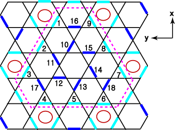
Figure 1: (Color online) Dimer covering pattern for the valence bond solid phase with a 36-site unit cell. The unit cell with 36 sites (or 18 dimers) is indicated by the enclosing dotted line. Thick solid bars denote singlet dimers. We use numbers between 1 and 9 to represent surrounding dimers (light-blue bars) while core dimers (dark-blue bars) are denoted by numbers between 10 and 18. Red circles indicate the locations of perfect hexagons. Note that perfect hexagons are made of three neighboring dimers, $(1,4,7)$ or $(3,6,9)$. The dimers 2, 5, and 8 become bridges connecting perfect hexagons.

In this paper, we focus on the valence bond solid ground state with a 36-site unit cell (shown in Fig. 1) and compute spin-triplet excitation spectra by using bond opertor formalism. The triplet excitation spectra can be directly measured in future neutron scattering experiments when single crystals become available. The eighteen dimers in a 36-site unit cell can be categorized into two groups: “core” dimers (numbered $10-18$ in Fig. 1) including a “pin-wheel” structure at the center and “surrounding” dimers (numbered $1-9$ in Fig. 1) including the honeycomb-lattice structure of “perfect hexagons”. As shown later, triplet excitations in the core dimers are highly localized and have flat dispersions. On the other hand, triplet excitations in the surrounding dimers can develop a dispersion by hopping around perfect hexagons.

Triplet excitation spectra are obtained by using the fully self-consistent mean-field theory in the bond operator representation. As shown later (see Fig.3 and Fig.6), the main feature of the triplet excitation spectra is that a large number of triplet modes are non-dispersive. The lowest triplet excitation is non-dispersive and degenerate with a dispersive mode at the zone center. Away from the zone center, the lowest triplet is separated from two other flat modes by a small energy gap. It is expected that the triplet excitation energies at high symmetric points such as $\Gamma$ and $X$ may be useful for comparison to future neutron scattering experiments on single crystals.

The mean-field energy of the ground state is $-0.427J$ which is not too bad for a näive mean-field theory when compared to $-0.438J$ obtained from exact diagonalization of a 36-site cluster Leung . On the other hand, the lowest spin-triplet gap is rather high, namely $0.795J$, which is expected to be significantly reduced once quantum fluctuations are properly taken into account. It is shown later that the formation of two-triplet bound state can renormalize the lowest spin-triplet gap from $0.795J$ to $0.622J$. While it is still larger than $0.164J$ obtained from exact diagonalization of a 36-site cluster Sindzingre , it is certainly in the right direction. Possible origins for the discrepancy are discussed later.

The rest of the paper is organized as follows. In section II, physical motivations for studying the VBS state with a 36-site unit cell are provided. In this section, the bond operator representation is explained. In section III, the bond operator mean-field theory is developed. Results for the spin-triplet excitation spectra and quantum fluctuation effects are presented in section IV. Finally, in section V we conclude by making a direct comparison between the lowest spin-triplet excitation obtained from our theory and those from the spin liquid theories. In the spin liquid states, triplet excitations form a continuum. The lower bound of such continuum, or the threshold energy, is given by the convolution of spinon-antispinon excitation spectra. Detailed measurement of the triplet spectra would be a key to the identification of the true ground state.

II Motivation for Valence Bond Solid

In this section we discuss physical motivations for the valence bond solid (VBS) state with a 36-site unit cell structure. The VBS state with a 36-site unit cell was initially proposed by Marston and Zeng Marston who envisioned the Kagome lattice as a honeycomb-lattice arrangement of perfect hexagons composed of resonant spin singlets.

Some time later, Nikolic and Senthil Nikolic provided an argument for the general validity of the 36-site VBS state in the Kagome-lattice antiferromagnet by a duality mapping. The main idea of this work is that the original Kagome-lattice antiferromagnetic model can be mapped to the fully frustrated Ising model on the dual dice lattice with transverse fields. Using a reasonable assumption about the magnitude of the transverse fields relative to the Ising coupling parameter, it is shown that the honeycomb structure of perfect hexagons is likely to be the ground state. Meanwhile, in a series expansion study by Singh and Huse Huse , it has been shown that the ground state energy is minimized when perfect hexagons are connected to their neighbors through empty triangles sharing a singlet dimer bond which in turn implies the same honeycomb structure of perfect hexagons as discussed in earlier works.

Here we provide an alternative viewpoint on the origin of the valence bond solid state. We begin by asking what state may be the most stable dimer covering configuration on the Kagome lattice. We argue that the most stable configuration is the dimer covering which maximizes the number of “topologically perpendicular” spin-singlet dimers. This argument is motivated by the exact ground state of the antiferromagnetic Heisenberg model on the Shastry-Sutherland lattice, where all dimers are mutually perpendicular to each other ss1 . We use the word “topologically perpendicular” since two neighboring dimers have the identical spin exchange energy as those obtained in the Shastry-Sutherland lattice when a spin belonging to a given dimer shares a triangle with its neighboring dimer.

It can be shown that the pinwheel structure at the core of the unit cell in Fig. 1 is the configuration maximizing the number of “topologically perpendicular” dimers. The rest of the dimer covering falls into the honeycomb array of perfect hexagons. While the final conclusion is exactly the same as before, there is an additional advantage over the previous arguments. Our point of view naturally leads to the fact that core dimers are decoupled from surrounding dimers. To see this, it is convenient to use a mathematical formalism which uses the spin-singlet degree of freedom as a natural building block of the VBS phase. The bond operator representation is such a formalism sachdev ; Gopalan ; kpark .

Let us consider two neighboring $S=\frac{1}{2}$ spins, ${\bf S}_{R}$ and ${\bf S}_{L}$. The Hilbert space is spanned by four states which can be decomposed into a singlet state, $|s\rangle$, and three triplet state, $|t_{x}\rangle$, $|t_{y}\rangle$ and $|t_{z}\rangle$. Then, singlet and triplet boson operators are introduced such that each of the above states can be created from the vacuum $|0\rangle$ as follows:

$$|s\rangle =s^{\dagger}|0\rangle=\frac{1}{\sqrt{2}}(|\uparrow\downarrow\rangle-|\downarrow\uparrow\rangle),$$

$$|t_{x}\rangle =t_{x}^{\dagger}|0\rangle=-\frac{1}{\sqrt{2}}(|\uparrow\uparrow\rangle-|\downarrow\downarrow\rangle),$$

$$|t_{y}\rangle =t_{y}^{\dagger}|0\rangle=\frac{i}{\sqrt{2}}(|\uparrow\uparrow\rangle+|\downarrow\downarrow\rangle),$$

$$|t_{z}\rangle =t_{z}^{\dagger}|0\rangle=\frac{1}{\sqrt{2}}(|\uparrow\downarrow\rangle+|\downarrow\uparrow\rangle).$$ (1)

To eliminate unphysical states from the enlarged Hilbert space, the following constraint needs to be imposed on the bond-particle Hilbert space:

$$s^{\dagger}s+t_{\alpha}^{\dagger}t_{\alpha}=1,$$ (2)

where $\alpha=x,y,$ and $z$, and we adopt the summation convention for the repeated index hereafter unless mentioned otherwise.

Constrained by this equation, the exact expressions for the spin operators can be written in terms of the bond operators.

$$S_{R\alpha} =\frac{1}{2}(s^{{\dagger}}t_{\alpha}+t_{\alpha}^{{\dagger}}s-i\varepsilon_{\alpha\beta\gamma}t_{\beta}^{{\dagger}}t_{\gamma}),$$

$$S_{L\alpha} =\frac{1}{2}(-s^{{\dagger}}t_{\alpha}-t_{\alpha}^{{\dagger}}s-i\varepsilon_{\alpha\beta\gamma}t_{\beta}^{{\dagger}}t_{\gamma}),$$ (3)

where $\varepsilon_{\alpha\beta\gamma}$ is the third rank antisymmetric tensor with $\varepsilon_{xyz}=1$.

When neighboring dimers are “topologically perpendicular”, spin-singlet contributions from both of the constituent spins of the neighboring dimer exactly cancel out. This cancellation can be seen in the bond operator representation of spin operators in Eq. (II) where it is shown that a pair of the spin operators within the same dimer have the opposite sign in the parts containing spin singlets. This results in the Hamiltonian with no dispersive quadratic part for core triplets, which eventually gives rise to nine-fold degenerate flat bands plotted in Fig. 3 and 6 in Sec. IV. This fact is completely consistent with conclusions from the series expansion studies Huse2 ; Huse .

In conclusion, the honeycomb lattice of perfect hexagons is a stable dimer covering maximizing the number of “topologically perpendicular” dimers, which in turn naturally suggests decoupling of core dimers from surrounding ones. Since the bond operator representation is a perfect theoretical framework for such situation, we use it to analyze the Kagome-lattice antiferromagnetic Heisenberg model.

Since we expect qualitatively different behaviors between core and surrounding dimers, we introduce a different set of parameters for their singlet condensate densities, $\langle s_{{\bf i},n}\rangle$ = $\bar{s}_{n}$ and chemical potentials, $\mu_{{\bf i},n}$. Here ${\bf i}$ denotes the position of the unit cell located at ${\bf i}$ and $n$ indicates the dimer index inside the unit cell. Furthermore, it is expected that the dynamics is different for the dimers within perfect hexagons (the dimers 1, 3, 4, 6, 7, and 9 in Fig. 1) and those bridging perfect hexagons (the dimers 2, 5, 8 in Fig. 1). Therefore, we introduce $\bar{s}_{C}$, $\mu_{C}$ for nine core dimers, $\bar{s}_{H}$, $\mu_{H}$ for six surrounding dimers of perfect hexagons, and $\bar{s}_{Br}$, $\mu_{Br}$ for three bridging dimers connecting perfect hexagons. Technical details of the bond operator analysis are provided in the next section. Readers who are only interested in the results may directly go to Sec. IV.

III Hamiltonian and the Mean Field Theory

We consider the following Hamiltonian for the Heisenberg model:

$$H_{J}=\sum_{\langle{\bf r},{\bf r}^{\prime}\rangle}J_{{\bf r},{\bf r}^{\prime}}{\bf S}({\bf r})\cdot{\bf S}({\bf r}^{\prime})$$ (4)

where ${\bf r}$ indicates the original coordinate of the lattice, $J_{{\bf r},{\bf r}^{\prime}}=J$ within dimers, and $J_{{\bf r},{\bf r}^{\prime}}=\lambda J$ between neighboring sites belonging to different dimers. Utilizing the bond operator representation of spin operators, the Hamiltonian can be rewritten solely in terms of bond particle operators. At this point the hard-core constraint among bond particle operators is imposed via the Lagrange multiplier method;

$$H_{\mu}=-\sum_{{\bf i},n}\mu_{{\bf i},n}(\bar{s}^{2}_{n}+t^{\dagger}_{{\bf i},n\alpha}t_{{\bf i},n\alpha}-1),$$ (5)

where $({\bf i},n)$ denotes the position of the $n$-th dimer in the unit cell located at ${\bf i}$. The chemical potential, $\mu_{{\bf i},n}$, is set to be $\mu_{C}$ for core dimers, $\mu_{H}$ for perfect hexagon dimers, and $\mu_{Br}$ for bridge dimers. Similarly, the spin-singlet condensate density, $\bar{s}_{n}$, is set to be $\bar{s}_{C}$ for core dimers, $\bar{s}_{H}$ for perfect hexagon dimers, and $\bar{s}_{Br}$ for bridge dimers.

The total Hamiltonian, $H=H_{J}+H_{\mu}$, can be written as follows:

$$H=N\epsilon_{0}+H_{\textrm{Quad, Core}}+H_{\textrm{Quad, Surrounding}}+H_{\textrm{Quartic}},$$ (6)

where $H_{\textrm{Quad, Core}}$ denotes the quadratic part of the Hamiltonian for core triplets while $H_{\textrm{Quad, Surrounding}}$ represents for surrounding triplets. In the above, $N$ is the number of unit cells and

$$\epsilon_{0} =9\left[\mu_{C}(1-{\bar{s}_{C}}^{2})-\frac{3}{4}J{\bar{s}_{C}}^{2}\right]$$

$$+6\left[\mu_{H}(1-{\bar{s}_{H}}^{2})-\frac{3}{4}J{\bar{s}_{H}}^{2}\right]$$

$$+3\left[\mu_{Br}(1-{\bar{s}_{Br}}^{2})-\frac{3}{4}J{\bar{s}_{Br}}^{2}\right].$$ (7)

It is important to note that the Hamiltonian does not have the coupling between core and surrounding triplets at the quadratic level. As shown in Sec. IV, the absence of quadratic coupling is crucial for a complete decoupling between core and surrounding triplets.

The quadratic Hamiltonian for core dimers is given by

$$H_{\textrm{Quad, Core}} =\left(\frac{J}{4}-\mu_{C}\right)\sum_{\textbf{k}}\sum_{n=10}^{18}t^{{\dagger}}_{n\alpha}(\textbf{k})t_{n\alpha}(\textbf{k}),$$ (8)

where $\alpha=x,y,$ and $z$. Also, the quadratic Hamiltonian for surrounding dimers is given by

$$H_{\textrm{Quad, Surrounding}} =H_{\textrm{Quad,0}}+H_{\textrm{Quad,A}}+H_{\textrm{Quad,B}}+H_{\textrm{Quad,C}}$$ (9)

where $H_{\textrm{Quad,0}}$ denotes the quadratic Hamiltonian of triplet operators within a unit cell. $H_{\textrm{Quad,A}}$, $H_{\textrm{Quad,B}}$, and $H_{\textrm{Quad,C}}$ describe quadratic coupling between a given unit cell and neighboring unit cells separated by displacement vectors, ${\bf r}_{A}$, ${\bf r}_{B}$, and ${\bf r}_{C}$, respectively. These displacement vectors are defined as follows:

$${\bf r}_{A} =4\sqrt{3}a\hat{x},$$

$${\bf r}_{B} =2\sqrt{3}a\hat{x}-6a\hat{y},$$

$${\bf r}_{C} =\textbf{${\bf r}_{B}$}-\textbf{${\bf r}_{A}$}=-2\sqrt{3}a\hat{x}-6a\hat{y},$$ (10)

where $a$ is the distance between nearest neighbor spins. More explicitly, we get

$$H_{\textrm{Quad,0}}=\left(\frac{J}{4}-\mu_{H}\right)\sum_{\textbf{k}}\sum_{n\in g_{H}}t^{{\dagger}}_{n\alpha}(\textbf{k})t_{n\alpha}(\textbf{k})$$

$$\qquad+\left(\frac{J}{4}-\mu_{Br}\right)\sum_{\textbf{k}}\sum_{n\in g_{Br}}t^{{\dagger}}_{n\alpha}(\textbf{k})t_{n\alpha}(\textbf{k})$$

$$+\frac{{\bar{s}_{H}\bar{s}_{Br}}\lambda J}{4}\sum_{(m,n)\in G_{s}}\sum_{\textbf{k}}\Big{\{}[t^{{\dagger}}_{m\alpha}(\textbf{k})t_{n\alpha}(\textbf{k})+\textrm{H. c.}]$$

$$\qquad\qquad\qquad+[t^{{\dagger}}_{m\alpha}(\textbf{k})t^{{\dagger}}_{n\alpha}(-\textbf{k})+\textrm{H. c.}]\Big{\}}$$ (11)

with $g_{H}=\{1,4,7,3,6,9\}$, $g_{Br}=\{2,5,8\}$, and $G_{S}=\{(1,2),(2,3),(4,5),(5,6),(7,8),(8,9)\}$. Furthermore,

$$H_{\textrm{Quad,A}}=$$

$$-\frac{{\bar{s}_{H}}^{2}\lambda J}{4}\sum_{(m,n)\in G_{A,H}}\sum_{\textbf{k}}\Big{\{}[e^{i{\bf k}\cdot{\bf r}_{A}}t^{{\dagger}}_{m\alpha}(\textbf{k})t_{n\alpha}(\textbf{k})+\textrm{H. c.}]$$

$$\qquad\qquad\qquad+[e^{i{\bf k}\cdot{\bf r}_{A}}t^{{\dagger}}_{m\alpha}(\textbf{k})t^{{\dagger}}_{n\alpha}(-\textbf{k})+\textrm{H. c.}]\Big{\}}$$

$$-\frac{{\bar{s}_{H}\bar{s}_{Br}}\lambda J}{4}\sum_{(m,n)\in G_{A,Br}}\sum_{\textbf{k}}\Big{\{}[e^{i{\bf k}\cdot{\bf r}_{A}}t^{{\dagger}}_{m\alpha}(\textbf{k})t_{n\alpha}(\textbf{k})+\textrm{H. c.}]$$

$$\qquad\qquad\qquad+[e^{i{\bf k}\cdot{\bf r}_{A}}t^{{\dagger}}_{m\alpha}(\textbf{k})t^{{\dagger}}_{n\alpha}(-\textbf{k})+\textrm{H. c.}]\Big{\}},$$ (12)

where

$$G_{A,H}=\{(1,4),(9,6)\},\quad G_{A,Br}=\{(1,5),(9,5)\}.$$ (13)

$H_{\textrm{Quad,B}}$ and $H_{\textrm{Quad,C}}$ can be obtained from $H_{\textrm{Quad,A}}$ by replacing (i) ${\bf r}_{A}$ by ${\bf r}_{B}$ and ${\bf r}_{C}$ and (ii) $(G_{A,H},G_{A,Br})$ by $(G_{B,H},G_{B,Br})$ and $(G_{C,H},G_{C,Br})$, respectively. Here,

$$G_{B,H} =\{(9,3),(7,4)\},\quad G_{B,Br}=\{(8,3),(8,4)\},$$

$$G_{C,H} =\{(7,1),(6,3)\},\quad G_{C,Br}=\{(7,2),(6,2)\}.$$ (14)

The quartic interaction part of the Hamiltonian is analyzed in the Hartree-Fock mean-field theory via quadratic decoupling. The resulting mean-field Hamiltonian is written as follows:

$$H_{\textrm{Quartic}} =H_{\textrm{Quartic,0}}+H_{\textrm{Quartic,A}}+H_{\textrm{Quartic,B}}+H_{\textrm{Quartic,C}}$$ (15)

where, similar to the quadratic counterparts, $H_{\textrm{Quartic,0}}$ denotes the quartic Hamiltonian of triplet operators within a unit cell. $H_{\textrm{Quartic,A}}$, $H_{\textrm{Quartic,B}}$, and $H_{\textrm{Quartic,C}}$ describe quartic coupling between a given unit cell and neighboring unit cells separated by displacement vectors, ${\bf r}_{A}$, ${\bf r}_{B}$, and ${\bf r}_{C}$, respectively. More explicitly, we obtain

$$H_{\textrm{Quartic,0}}=\frac{9}{2}\lambda J(Q_{C}^{2}-P_{C}^{2}+Q_{CS}^{2}-P_{CS}^{2})$$

$$+\frac{3}{2}\lambda J(Q_{H}^{2}-P_{H}^{2})+\frac{3}{2}\lambda J(Q_{Br1}^{2}-P_{Br1}^{2}+Q_{Br2}^{2}-P_{Br2}^{2})$$

$$+\frac{\lambda J}{4}\sum_{(m,n)\in G_{S}}\sum_{\textbf{k}}\Big{\{}[P_{Br1}t^{{\dagger}}_{m\alpha}(\textbf{k})t_{n\alpha}(\textbf{k})+\textrm{H. c.}]$$

$$\qquad\qquad\qquad-[Q_{Br1}t^{{\dagger}}_{m\alpha}(\textbf{k})t^{{\dagger}}_{n\alpha}(-\textbf{k})+\textrm{H. c.}]\Big{\}}$$

$$+\frac{\lambda J}{2}\sum_{(m,n)\in G_{C}}\sum_{\textbf{k}}\Big{\{}[P_{C}t^{{\dagger}}_{m\alpha}(\textbf{k})t_{n\alpha}(\textbf{k})+\textrm{H. c.}]$$

$$\qquad\qquad\qquad-[Q_{C}t^{{\dagger}}_{m\alpha}(\textbf{k})t^{{\dagger}}_{n\alpha}(-\textbf{k})+\textrm{H. c.}]\Big{\}}$$

$$+\frac{\lambda J}{2}\sum_{(m,n)\in G_{CS}}\sum_{\textbf{k}}\Big{\{}[P_{CS}t^{{\dagger}}_{m\alpha}(\textbf{k})t_{n\alpha}(\textbf{k})+\textrm{H. c.}]$$

$$\qquad\qquad\qquad-[Q_{CS}t^{{\dagger}}_{m\alpha}(\textbf{k})t^{{\dagger}}_{n\alpha}(-\textbf{k})+\textrm{H. c.}]\Big{\}}$$ (16)

where

$$G_{C} =\{(10,11),(11,12),(12,13),(13,14),(14,15),$$

$$\qquad(15,10),(10,16),(12,17),(14,18)\},$$

$$G_{CS} =\{(16,1),(16,9),(17,4),(17,3),(18,7),(18,6),$$

$$\qquad(11,2),(13,5),(15,8)\}.$$ (17)

One also gets

$$H_{\textrm{Quartic,A}}$$

$$=\frac{\lambda J}{4}\sum_{(m,n)\in G_{A,H}}\sum_{\textbf{k}}\Big{\{}[P_{H}e^{i{\bf k}\cdot{\bf r}_{A}}t^{{\dagger}}_{m\alpha}(\textbf{k})t_{n\alpha}(\textbf{k})+\textrm{H. c.}]$$

$$\qquad\qquad\qquad-[Q_{H}e^{i{\bf k}\cdot{\bf r}_{A}}t^{{\dagger}}_{m\alpha}(\textbf{k})t^{{\dagger}}_{n\alpha}(-\textbf{k})+\textrm{H. c.}]\Big{\}}$$

$$+\frac{\lambda J}{4}\sum_{(m,n)\in G_{A,Br}}\sum_{\textbf{k}}\Big{\{}[P_{Br2}e^{i{\bf k}\cdot{\bf r}_{A}}t^{{\dagger}}_{m\alpha}(\textbf{k})t_{n\alpha}(\textbf{k})+\textrm{H. c.}]$$

$$\qquad\qquad\qquad-[Q_{Br2}e^{i{\bf k}\cdot{\bf r}_{A}}t^{{\dagger}}_{m\alpha}(\textbf{k})t^{{\dagger}}_{n\alpha}(-\textbf{k})+\textrm{H. c.}]\Big{\}},$$ (18)

Similar to the quadratic case, $H_{\textrm{Quartic,B}}$ and $H_{\textrm{Quartic,C}}$ can be obtained from $H_{\textrm{Quartic,A}}$ by replacing (i) ${\bf r}_{A}$ by ${\bf r}_{B}$ and ${\bf r}_{C}$ and (ii) $(G_{A,H},G_{A,Br})$ by $(G_{B,H},G_{B,Br})$ and $(G_{C,H},G_{C,Br})$, respectively.

The above mean-field order parameters, $P_{H}$, $Q_{H}$, $P_{Br1}$, $Q_{Br1}$, $P_{Br2}$, $Q_{Br2}$, $P_{C}$, $Q_{C}$, $P_{CS}$, and $Q_{CS}$, are determined by solving a coupled set of ten self-consistency equations. In other words,

$$P_{\gamma} \equiv\langle t^{{\dagger}}_{{\bf i},n\alpha}t_{{\bf j},m\alpha}\rangle,\;\;Q_{\gamma}\equiv\langle t_{{\bf i},n\alpha}t_{{\bf j},m\alpha}\rangle$$

where $({\bf i},{\bf j})$ indicates the positions of the neighboring unit cells and $\gamma\in(C,H,Br1,Br2,CS)$, both of which are related to the dimer index pair, $(n,m)$. To be specific, if $(n,m)\in G_{C}$, $\gamma=C$ and ${\bf j}={\bf i}$. If $(n,m)\in G_{S}$, $\gamma=Br1$ and ${\bf j}={\bf i}$. On the other hand, if $(n,m)\in G_{A,H}$, $\gamma=H$ and ${\bf j}-{\bf i}={\bf r}_{A}$. Those for $G_{B,H}$ and $G_{C,H}$ are defined similarly. Also, if $(n,m)\in G_{A,Br}$, $\gamma=Br2$ and ${\bf j}-{\bf i}={\bf r}_{A}$. Those for $G_{B,Br}$ and $G_{C,Br}$ are defined similarly. Finally, if $(n,m)\in G_{CS}$, $\gamma=CS$ and ${\bf j}={\bf i}$.

In physical terms, $P_{C}$ and $Q_{C}$ describe the diagonal and off-diagonal triplet correlations between core dimers, respectively. In the case of surrounding dimers, six order parameters are introduced. First, $P_{H}$ and $Q_{H}$ denote correlations between dimers within perfect hexagons. The other four order parameters, $(P_{Br1},Q_{Br1})$ and $(P_{Br2},Q_{Br2})$, represent correlations between a bridge dimer and two neighboring dimers belonging to the nearby perfect hexagons. In particular, $(P_{Br1},Q_{Br1})$ describes the correlations between a given bridge dimer and the dimer lying inside the nearby perfect hexagon in its parallel direction. $(P_{Br2},Q_{Br2})$ denotes the other correlations. A schematic diagram showing the definition of these order parameters is provided in the top panel of Fig.2. Finally, $P_{CS}$ and $Q_{CS}$ indicate the correlations between core and surrounding dimers.

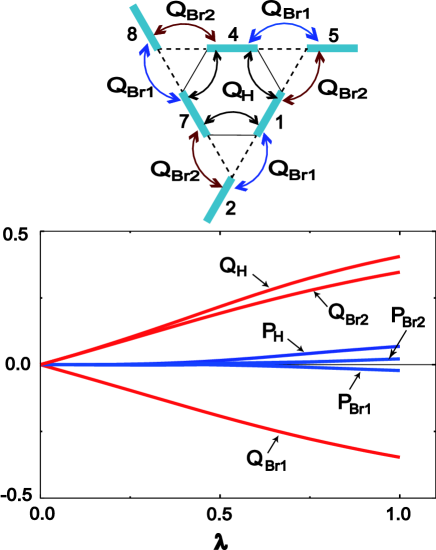
Figure 2: (Color online) Mean-field order parameters, $P$ and $Q$, as a function of $\lambda$. The top figure depicts dimer covering of the valence bond solid state in the vicinity of a perfect hexagon, which also shows how various $Q$’s are defined. Note that each $Q$ describes an off-diagonal correlation between two dimers connected by corresponding arrows. Diagonal correlations, $P_{H}$, $P_{Br1}$, and $P_{Br2}$, are defined in the same way. It is interesting to note that $Q_{Br1}$ $(P_{Br1})$ and $Q_{Br2}$ $(P_{Br2})$ have opposite signs.

In order to determine the ten mean-field order parameters defined above, one needs to compute yet another six unknown parameters which are three spin-singlet condensate densities, $\bar{s}_{C}$, $\bar{s}_{H}$, and $\bar{s}_{Br}$, and three chemical potentials, $\mu_{C}$, $\mu_{H}$, and $\mu_{Br}$. The hard-core constraints for bond operators provide three equations:

$$\bar{s}_{C}^{2}=1-\frac{1}{9N}\sum_{n=10}^{18}\sum_{\textbf{k}}\langle t^{{\dagger}}_{n\alpha}(\textbf{k})t_{n\alpha}(\textbf{k})\rangle,$$

$$\bar{s}_{H}^{2}=1-\frac{1}{6N}\sum_{n\in g_{H}}\sum_{\textbf{k}}\langle t^{{\dagger}}_{n\alpha}(\textbf{k})t_{n\alpha}(\textbf{k})\rangle,$$

$$\bar{s}_{Br}^{2}=1-\frac{1}{3N}\sum_{n\in g_{Br}}\sum_{\textbf{k}}\langle t^{{\dagger}}_{n\alpha}(\textbf{k})t_{n\alpha}(\textbf{k})\rangle.$$ (20)

On the other hand, the energy minimization with respect to spin-singlet condensate densities generate the other three necessary equations:

$$\frac{\partial\varepsilon_{gr}}{\partial\bar{s}_{C}}=0,\quad\frac{\partial\varepsilon_{gr}}{\partial\bar{s}_{H}}=0,\quad\frac{\partial\varepsilon_{gr}}{\partial\bar{s}_{Br}}=0.$$ (21)

Now the ground state energy and excitation spectra can be obtained as follows. For this purpose, the mean-field Hamiltonian is rewritten in the following compact fashion:

$$H=\frac{1}{2}\sum_{\textbf{k}}{\bf\Lambda}_{\alpha}^{{\dagger}}{\bf M}{\bf\Lambda}_{\alpha}-\frac{3}{4}\textrm{Tr}{\bf M},$$ (22)

where

$${\bf\Lambda}_{\alpha}^{\dagger}(\textbf{k}) \equiv\left[t^{{\dagger}}_{1\alpha}(\textbf{k}),\ldots,t^{{\dagger}}_{18\alpha}(\textbf{k}),t_{1\alpha}(-\textbf{k}),\ldots,t_{18\alpha}(-\textbf{k})\right]$$ (23)

and the matrix, ${\bf M}$, is determined by simply reorganizing the mean-field Hamiltonian.

It is important to note that our Hamiltonian describes dynamics of boson operators, in which case obtaining normal modes of the Hamiltonian is not equivalent to diagonalizing the matrix ${\bf M}$ in the above. Instead, we need to consider the following eigenvalue problem Blaizot :

$${\bf I}_{B}{\bf M}{\bf\Psi}=\omega{\bf\Psi}$$ (24)

where

$${\bf I}_{B}=\left(\begin{array}[]{ccc}{\bf I}&{\bf 0}\\ {\bf 0}&-{\bf I}\\ \end{array}\right)$$ (27)

with ${\bf I}$ being the $18\times 18$ identity matrix and

$${\bf\Psi}=\left(\begin{array}[]{ccc}{\bf\eta}\\ {\bf\xi}\\ \end{array}\right)$$ (30)

with ${\bf\eta}^{t}=(\eta_{1},\ldots,\eta_{18})$ and ${\bf\xi}^{t}=(\xi_{1},\ldots,\xi_{18})$. This difference between fermionic and bosonic problems fundamentally originates from the difference in their operator commutation relations.

IV Results

IV.1 Ground state energy

The ground state energy per unit cell is obtained by solving the eigenvalue equation described in the preceding section. In other words,

$$\varepsilon_{gr} =\epsilon_{0}+\frac{9}{2}\lambda J(Q_{C}^{2}-P_{C}^{2}+Q_{CS}^{2}-P_{CS}^{2})$$

$$\qquad+\frac{3}{2}\lambda J(Q_{H}^{2}-P_{H}^{2})$$

$$\qquad+\frac{3}{2}\lambda J(Q_{Br1}^{2}-P_{Br1}^{2}+Q_{Br2}^{2}-P_{Br2}^{2})$$

$$\qquad+\frac{3}{2}\frac{1}{N}\sum_{\textbf{k}}\sum_{n=1}^{18}\omega_{n}(\textbf{k})-\frac{18}{2}\Big{(}\frac{J}{4}-\mu_{H}\Big{)}$$

$$\qquad-\frac{9}{2}\Big{(}\frac{J}{4}-\mu_{Br}\Big{)}-\frac{27}{2}\Big{(}\frac{J}{4}-\mu_{C}\Big{)},$$ (31)

where $\omega_{n}$ $(n=1,\dots,18)$ are triplet eigenenergies obtained from diagonalization. As mentioned previously, the ground state energy is minimized with respect to spin-singlet condensate densities. Note that the minimization process is performed simultaneously satisfying the ten self-consistency conditions and three hard-core constraints.

Now let us discuss numerical results. When quartic interactions are completely ignored, the ground state energy per site is found to be $-0.414J$ at $\lambda=1$. The inclusion of quartic interactions lowers the ground state energy to $-0.427J$ per site, which can be favorably compared with $-0.438J$ from exact diagonalization Leung . This result is quite encouraging given that it is obtained from a naive mean-field theory. This perhaps indicates the robustness of the VBS state.

IV.2 Triplet dispersions without quartic interactions

We now discuss the energy dispersion of triplet excitations. In this section quartic interaction terms are ignored. The analysis of quartic interaction effects is relegated to the next section. One of the reasons why we first focus on the quadratic part of the Hamiltonian is that the overall structure of the dispersion is well captured even at the quadratic level. The inclusion of quartic interaction terms modifies the dispersion only quantitatively.

As seen in Eq. (8), core triplets have no dispersions. In this situation the ground-state energy minimization condition immediately leads to the conclusion that $\bar{s}_{C}=1$ and $\mu_{C}=-0.75J$, which implies that in the core part of the unit cell triplet fluctuations are entirely absent and triplet excitations are completely localized. As mentioned previously, the reason for this complete localization has to do with the dimer covering structure of the valence bond solid phase. The key fact is that every core dimer is “topologically perpendicular” to its neighboring dimers in the sense that each spin belonging to a core dimer shares a triangle with its neighboring dimer. This results in the Hamiltonian with no dispersive quadratic part for core triplets, which gives rise to nine-fold degenerate flat bands plotted as a dotted line in Fig. 3.

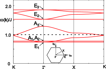
Figure 3: (Color online) Energy dispersion of the triplet excitations when quartic interaction effects are ignored. The dotted line describes the nine-fold degenerate triplet states from core dimers. The solid lines denote the nine triplet states from surrounding dimers.

Now let us turn to the remaining nine triplets in the surrounding dimers. After diagonalizing the corresponding bosonic Hamiltonian via the method described in the preceding section, mean-field parameters, $\bar{s}_{H}$,$\bar{s}_{Br}$, $\mu_{H}$, and $\mu_{Br}$, are self-consistently determined. Fig. 3 shows the resulting dispersion of nine triplet excitations at the isotropic exchange limit of $\lambda=1$. It is convenient at this point to classify characteristics of these eigenmodes using group theory. Since the unit cell possesses the $C_{3}$ point group symmetry, the states at the $\Gamma$ point can be decomposed with respect to irreducible representations of the $C_{3}$ point group. A representation, $R$, can be decomposed in the basis containing nine triplets localized at each dimer as follows:

$$R=3A\bigoplus 3E$$ (32)

where $A$ is an one-dimensional representation and $E$ is a two-dimensional one. (See Ref. Tinkham, for standard conventions and notations.)

The lowest flat mode belonging to the E irreducible representation is degenerate with a dispersive mode at the $\Gamma$ point ($E_{1}$ mode in Fig.3). There are two other flat modes ($A_{1}$ and $A_{2}$) which are separated from the lowest flat mode by a small gap. These states have $A$ characters and are completely localized within perfect hexagons. The fifth dispersive mode ($A_{3}$) is another $A$ mode. The remaining four modes belong to the E irreducible representation and make two doubly degenerate states at the $\Gamma$ point ($E_{2}$ and $E_{3}$). Real space representations of the five flat mode eigenvectors are shown in Fig. 4 and 5. Details of these eigenvectors for non-dispersive modes are further analyzed in the next section where their explicit forms are also presented. In the next section we study quartic interaction effects via the self-consistent mean-field theory.

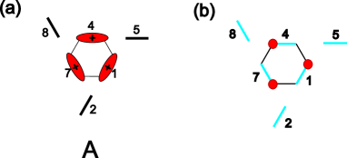
Figure 4: (Color online) Real space representation of the eigenvectors of the flat A mode at the $\Gamma$ point. The size of ovals and the sign inside indicate relative weights and phases of the amplitude at each dimer, respectively. (a) One of the flat $A$ modes with the energy eigenvalue $\Omega_{A}$. Triplets around each perfect hexagon have the same phases and weights. Two different flat $A$ modes are distinguished by relative phases between neighboring perfect hexagons. (b) Local geometry around a perfect hexagon. Here red dots indicate the position of R-spins within a dimer. See Eq. (II) for the definition of the R-spin.

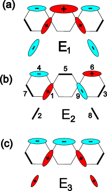
Figure 5: (Color online) Real space representation of the eigenvectors of the flat E modes. To avoid degeneracy eigenvectors are computed slightly away from the $\Gamma$ point to the direction of the K point, for (a) $E_{1}$ mode, (b) $E_{2}$ mode, and (c) $E_{3}$ mode. Note that the size of ovals and the sign indicate relative weights and phases of the amplitude at each dimer, respectively.

IV.3 Triplet dispersions with quartic interactions

In this section we solve the total Hamiltonian containing contributions from all eighteen dimers in the unit cell. The fully self-consistent calculation, however, shows that core dimers are still completely decoupled from surrounding dimers and remain flat in energy. In other words,

$$P_{C}=Q_{C}=P_{CS}=Q_{CS}=0,\quad\bar{s}_{C}=1,\quad\mu_{C}=-0.75J.$$ (33)

On the other hand, surrounding dimers experience band renormalization due to finite triplet correlations, $P$ and $Q$. Order parameters for the triplet correlations are plotted as a function of $\lambda$ in Fig.2. The order parameters are shown to have the largest value inside perfect hexagons which in turn implies that vacuum fluctuation is strongest at this location. Triplet correlations between bridge and perfect hexagon dimers are also quite large, about $86\%$ of those between perfect hexagon dimers. It is interesting to note that $Q_{Br1}$ $(P_{Br1})$ and $Q_{Br2}$ $(P_{Br2})$ are the same in magnitude but are the opposite in sign. In Fig.6 we plot the triplet dispersions obtained from fully self-consistent parameters at $\lambda=1$. The overall structure is identical to that obtained by ignoring quartic interaction terms.

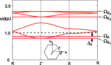
Figure 6: (Color online) Energy dispersion of the triplet excitations when quartic interaction effects are included in the self-consistent mean-field theory. Away from the zone center, the lowest flat mode is separated from doubly-degenerate flat $A$ modes by a small gap, $\Delta_{0}$ $\cong$ 0.069 J. Eigenenergies of the flat modes are shown on the right hand side of the plot, where subscripts indicate the irreducible representation of each state at the $\Gamma$ point.

One of the most interesting characteristics of the triplet dispersion is the existence of a large number of flat bands. Among the nine modes coming from surrounding dimers, five states have no dispersion. (If one includes the flat modes originating from core dimers, fourteen states out of eighteen are flat in energy.) These five flat modes are categorized in terms of the $C_{3}$ point group symmetry at the $\Gamma$ point. In the right hand side of Fig.6, each mode is indicated by $\Omega_{A_{1}}$, $\Omega_{A_{2}}$, $\Omega_{E_{1}}$, $\Omega_{E_{2}}$, and $\Omega_{E_{3}}$, respectively (these are also energy eigenvalues). Note that $\Omega_{A}$ = $\Omega_{A_{1}}$ = $\Omega_{A_{2}}$ and $\Omega_{E_{1}}$ $<$ $\Omega_{E_{2}}$ $<$ $\Omega_{E_{3}}$. In the above notations subscripts denote irreducible representations to which each flat mode belongs.

It is interesting to note that the eigenvalue equation can be solved exactly for the flat modes. The precise analytic expressions for the flat mode eigenvalues are given as follows:

$$\Omega_{A_{1}} =\Omega_{A_{2}}=\sqrt{(a_{H}-2b_{H})^{2}-4q_{H}^{2}},$$

$$\Omega_{E_{2}} =\sqrt{(a_{H}+b_{H})^{2}-q_{H}^{2}},$$

$$\Omega_{E_{1}} =\Omega_{-},\quad\Omega_{E_{3}}=\Omega_{+},$$ (34)

where

$$\Omega_{\pm}^{2}=\frac{1}{2}\left[a_{Br}^{2}+(a_{H}+b_{H})^{2}-q_{H}^{2}-12(q_{Br}^{2}-b_{Br}^{2})\pm\sqrt{D}\right],$$ (35)

$$D =\left[a_{Br}^{2}-(a_{H}+b_{H})^{2}+q_{H}^{2}\right]^{2}$$

$$-24(q_{Br}^{2}-b_{Br}^{2})\left[a_{Br}^{2}+(a_{H}+b_{H})^{2}-q_{H}^{2}\right]$$

$$+24a_{Br}\Big{[}(q_{Br}+b_{Br})^{2}(a_{H}+b_{H}-q_{H})$$

$$+(q_{Br}-b_{Br})^{2}(a_{H}+b_{H}+q_{H})\Big{]},$$ (36)

and

$$a_{H} =\frac{J}{4}-\mu_{H},\quad a_{Br}=\frac{J}{4}-\mu_{Br},$$

$$b_{H} =\frac{\lambda J}{4}(\bar{s}_{H}^{2}-P_{H}),\quad b_{Br}=\frac{\lambda J}{4}(\bar{s}_{H}\bar{s}_{Br}-P_{Br2}),$$

$$q_{H} =\frac{\lambda J}{4}(\bar{s}_{H}^{2}+Q_{H}),\quad q_{Br}=\frac{\lambda J}{4}(\bar{s}_{H}\bar{s}_{Br}+Q_{Br2}).$$ (37)

It is important to notice that the eigenvalues, $\Omega_{A_{1}}$, $\Omega_{A_{2}}$, and $\Omega_{E_{2}}$, are completely determined by the parameters defined inside perfect hexagons. In fact, the same energy eigenvalues are obtained by applying the bond operator theory to a single isolated perfect hexagon using the mean-field order parameters, $\mu_{H}$, $\bar{s}_{H}$, $P_{H}$, and $Q_{H}$. This means that for the flat $A$ and $E_{2}$ modes a simple product of perfect-hexagon eigenstates becomes that of the full Kagome lattice, at least in the self-consistent mean-field theory.

As mentioned in the previous section, the flat $A$ modes are completely localized within perfect hexagons, i. e. , there is no weight for the bridge dimers. Here triplets around each perfect hexagon have the same weight and phase while the $A_{1}$ and $A_{2}$ modes are distinguished by a relative phase difference in neighboring perfect hexagons. The $E_{2}$ mode is also localized within perfect hexagons. The difference between the flat $A$ and $E_{2}$ modes originates from the fact that they represent different eigenstates of the isolated perfect-hexagon. Schematic diagrams for the real space representation of these flat modes are provided in Fig. 4 and 5, which show the relative weight and sign of the eigenvector amplitudes at each real space dimer location.

To understand the flat nature of the $A$ modes, one needs to examine the local geometry around a perfect hexagon which is plotted in Fig. 4(b). As seen in Eq. (II), two constituent spins, the $R$ and $L$ spins, within the same dimer are distinguished by the sign difference in the part containing spin singlet operators. This is basically due to the odd parity of the spin singlet under the inversion with respect to the center of the dimer. The $R$-spins are denoted by red dots in Fig. 4(b). Because of the three-fold rotational symmetry, every spin from bridge dimers is simultaneously connected to both $R$ and $L$ spins of the perfect hexagon dimers. Due to the above-mentioned sign difference, hopping amplitudes between perfect hexagon and bridge dimers cancel, leading to the complete localization within perfect hexagons. The flat $E_{2}$ mode can be understood similarly.

We now present precise analytic expressions for the eigenvectors of all five flat modes in Table 1. The prefactors, $\tau_{M}$, in Table 1 denote the relative magnitudes of the hole (particle) component in the Bogoliubov quasiparticles (quasiholes), which are given as follows:

$$\tau_{A_{1}} =\tau_{A_{2}}=\frac{a_{H}-2b_{H}-\Omega_{H}}{2q_{H}},$$

$$\tau_{E_{2}} =\frac{\Omega_{E_{2}}-a_{H}-b_{H}}{q_{H}},$$

$$\tau_{E_{1}} =\frac{(\Omega_{E_{1}}^{2}-a_{Br}^{2})(\Omega_{E_{1}}-a_{H}-b_{H})}{q_{H}(\Omega_{E_{1}}^{2}-a_{Br}^{2})+12a_{Br}b_{Br}q_{Br}}$$

$$-\frac{\Big{\{}6\Omega_{E_{1}}(b_{Br}^{2}-q_{Br}^{2})+6a_{Br}(b_{Br}^{2}+q_{Br}^{2})\Big{\}}}{q_{H}(\Omega_{E_{1}}^{2}-a_{Br}^{2})+12a_{Br}b_{Br}q_{Br}},$$

$$\tau_{E_{3}} =\frac{(\Omega_{E_{3}}^{2}-a_{Br}^{2})(\Omega_{E_{3}}-a_{H}-b_{H})}{q_{H}(\Omega_{E_{3}}^{2}-a_{Br}^{2})+12a_{Br}b_{Br}q_{Br}}$$

$$-\frac{\Big{\{}6\Omega_{E_{3}}(b_{Br}^{2}-q_{Br}^{2})+6a_{Br}(b_{Br}^{2}+q_{Br}^{2})\Big{\}}}{q_{H}(\Omega_{E_{3}}^{2}-a_{Br}^{2})+12a_{Br}b_{Br}q_{Br}}.$$ (38)

Note that $\tau_{A_{1}}$, $\tau_{A_{2}}$ and $\tau_{E_{2}}$ depend only on the perfect hexagon parameters. The coefficients, $c_{1}$ $(d_{1})$ and $c_{3}$ $(d_{3})$ indicate the relative magnitude of coupling between perfect hexagon and bridge dimers in the $E_{1}$ and $E_{3}$ modes, respectively. More explicitly, one obtains

$$c_{1} =\frac{\Omega_{E_{1}}-a_{Br}}{b_{Br}+\tau_{E_{1}}q_{Br}},\quad d_{1}=\frac{-\Omega_{E_{1}}-a_{Br}}{b_{Br}+q_{Br}/\tau_{E_{1}}},$$

$$c_{3} =\frac{\Omega_{E_{3}}-a_{Br}}{b_{Br}+\tau_{E_{3}}q_{Br}},\quad d_{3}=\frac{-\Omega_{E_{3}}-a_{Br}}{b_{Br}+q_{Br}/\tau_{E_{3}}}.$$ (39)

Note that the eigenvector amplitudes in bridge dimers, i. e. , $(\eta_{2},\eta_{5},\eta_{8})$ and $(\xi_{2},\xi_{5},\xi_{8})$, are zero for the flat $A_{1}$, $A_{2}$ and $E_{2}$ modes, which confirms that they are completely localized within perfect hexagons.

	$A_{1}$	$A_{2}$	$E_{1}$	$E_{2}$	$E_{3}$
$\eta_{1}$	$z_{1}^{*}z_{2}$	$z_{1}^{*}z_{2}$	$2-z_{1}^{*}-z_{1}^{*}z_{2}$	$2-z_{1}^{*}-z_{1}^{*}z_{2}$	$2-z_{1}^{*}-z_{1}^{*}z_{2}$
$\eta_{4}$	$z_{2}$	$z_{2}$	$2-z_{1}-z_{2}$	$2-z_{1}-z_{2}$	$2-z_{1}-z_{2}$
$\eta_{7}$	$1$	$1$	$2-z_{2}^{*}-z_{2}^{*}z_{1}$	$2-z_{2}^{*}-z_{2}^{*}z_{1}$	$2-z_{2}^{*}-z_{2}^{*}z_{1}$
$\eta_{2}$	$0$	$0$	$c_{1}(1-z_{2}z_{1}^{*})$	$0$	$c_{3}(1-z_{2}z_{1}^{*})$
$\eta_{5}$	$0$	$0$	$c_{1}(1-z_{1})$	$0$	$c_{3}(1-z_{1})$
$\eta_{8}$	$0$	$0$	$c_{1}(1-z_{2}^{*})$	$0$	$c_{3}(1-z_{2}^{*})$
$\eta_{3}$	$r_{1}z_{2}$	$r_{2}z_{2}$	$2-z_{2}-z_{1}^{*}z_{2}$	$z_{2}+z_{1}^{*}z_{2}-2$	$2-z_{2}-z_{1}^{*}z_{2}$
$\eta_{6}$	$r_{1}z_{1}$	$r_{2}z_{1}$	$2-z_{1}-z_{2}^{*}z_{1}$	$z_{1}+z_{2}^{*}z_{1}-2$	$2-z_{1}-z_{2}^{*}z_{1}$
$\eta_{9}$	$r_{1}$	$r_{2}$	$2-z_{1}^{*}-z_{2}^{*}$	$z_{1}^{*}+z_{2}^{*}-2$	$2-z_{1}^{*}-z_{2}^{*}$
$\xi_{1}/\tau_{M}$	$z_{1}^{*}z_{2}$	$z_{1}^{*}z_{2}$	$2-z_{1}^{*}-z_{1}^{*}z_{2}$	$2-z_{1}^{*}-z_{1}^{*}z_{2}$	$2-z_{1}^{*}-z_{1}^{*}z_{2}$
$\xi_{4}/\tau_{M}$	$z_{2}$	$z_{2}$	$2-z_{1}-z_{2}$	$2-z_{1}-z_{2}$	$2-z_{1}-z_{2}$
$\xi_{7}/\tau_{M}$	$1$	$1$	$2-z_{2}^{*}-z_{2}^{*}z_{1}$	$2-z_{2}^{*}-z_{2}^{*}z_{1}$	$2-z_{2}^{*}-z_{2}^{*}z_{1}$
$\xi_{2}/\tau_{M}$	$0$	$0$	$d_{1}(1-z_{2}z_{1}^{*})$	$0$	$d_{3}(1-z_{2}z_{1}^{*})$
$\xi_{5}/\tau_{M}$	$0$	$0$	$d_{1}(1-z_{1})$	$0$	$d_{3}(1-z_{1})$
$\xi_{8}/\tau_{M}$	$0$	$0$	$d_{1}(1-z_{2}^{*})$	$0$	$d_{3}(1-z_{2}^{*})$
$\xi_{3}/\tau_{M}$	$r_{1}z_{2}$	$r_{2}z_{2}$	$2-z_{2}-z_{1}^{*}z_{2}$	$z_{2}+z_{1}^{*}z_{2}-2$	$2-z_{2}-z_{1}^{*}z_{2}$
$\xi_{6}/\tau_{M}$	$r_{1}z_{1}$	$r_{2}z_{1}$	$2-z_{1}-z_{2}^{*}z_{1}$	$z_{1}+z_{2}^{*}z_{1}-2$	$2-z_{1}-z_{2}^{*}z_{1}$
$\xi_{9}/\tau_{M}$	$r_{1}$	$r_{2}$	$2-z_{1}^{*}-z_{2}^{*}$	$z_{1}^{*}+z_{2}^{*}-2$	$2-z_{1}^{*}-z_{2}^{*}$

Table 1: Eigenvectors of the five flat modes. Among the 36 components of the full eigenvector, ${\bf\Psi}^{t}=(\eta_{1},\ldots,\eta_{18},\xi_{1},\ldots,\xi_{18})$, only the components for surrounding dimers are shown. Note that core dimers are decoupled from surrounding ones. In the above, $z_{1}=\exp{(-i{\bf k}\cdot{\bf r}_{A})}$, $z_{2}=\exp{(-i{\bf k}\cdot{\bf r}_{B})}$, and $(r_{1},r_{2})$ represents any pair of two complex numbers satisfying $r_{1}^{*}r_{2}=-1$. The prefactor, $\tau_{M}$, depends on the mode index, $M\in A_{1},A_{2},E_{1},E_{2},$ and $E_{3}$. Explicit expressions for $\tau_{M}$ as well as $c_{1},c_{3},d_{1},$ and $d_{3}$ are provided in the text.

While the amplitudes in bridge dimers do not vanish, the nature of the $E_{1}$ and $E_{3}$ modes is rather similar to that of the $E_{2}$ mode. As one can see from Table 1, the amplitudes inside perfect hexagons for the $E_{1}$ and $E_{3}$ modes are precisely identical to those for the $E_{2}$ mode. This identity is fundamentally due to (i) the odd parity of the singlet operator and (ii) the three-fold rotational symmetry of the lattice. Coupling to bridge dimers splits triple degeneracy by lowering the energy for the $E_{1}$ mode and increasing it for the $E_{3}$ mode. The difference from the $E_{2}$ mode case is that hopping amplitudes between perfect hexagon and bridge dimers do not cancel, but instead they add.

It is interesting to note that our $E_{1}$ mode is fully consistent with the lowest triplet excitation obtained in the series expansion study by Singh and Huse Huse2 . In fact, after properly redefining the unit cell convention, it can be shown that our $E_{1}$ mode becomes precisely equivalent to the lowest energy eigenstate obtained in first order of $\lambda$ under the conditions that (i) all off-diagonal coupling terms are ignored, (ii) all quartic interaction terms are ignored, and (iii) perfect hexagon and bridge dimers are physically identical, i. e., $\bar{s}_{H}=\bar{s}_{Br}$ and $\mu_{H}=\mu_{Br}$. Considering that our $E_{1}$ mode does not change abruptly upon relaxing these conditions or restoring the full self-consistency, one may expect that our $E_{1}$ mode is indeed adiabatically connected to the lowest energy eigenvector obtained in the previous series expansion study Huse2 and perhaps the corresponding eigenvector in yet-to-be-studied higher order series expansion.

IV.4 Quantum fluctuations

Up to now, triplet interactions are treated within the self-consistent mean-field theory. To investigate effects of quantum fluctuations, we need to go beyond the mean field theory. There are three classes of order parameters in the mean-field theory, which can be affected by quantum fluctuations. These are chemical potentials, $\mu$, diagonal correlation parameters, $P$, and off-diagonal correlation parameters, $Q$. Spin-singlet condensate densities, $\bar{s}$, which are the remaining variational parameters, can be determined by minimizing the ground state energy after quantum fluctuation effects are incorporated for the above-mentioned order parameters. Below we check how each of these order parameters is affected by quantum fluctuations.

The chemical potential is the Lagrange multiplier for the hard-core constraint. In the usual weak-coupling limit where the singlet nature of the ground state is robust, the dominant contribution comes from the hard-core constraint, Eq. (2), which can be conveniently implemented by an infinite on-site repulsion between triplets Kotov1 . When the triplet density is low, this hard-core constraint can be treated by summing ladder diagrams for the scattering vertex. The complete ladder diagram summation for the full lattice is rather complicated. Fortunately, however, in our system the most important aspect of the lowest excitation is determined by the nature of eigenstates inside a single perfect hexagon. Therefore, we expect that the dynamics inside a single perfect hexagon is a good indicator for the full lattice as far as the lowest excitation is concerned. It is shown that there is little difference between the chemical potential obtained from the mean-field theory and that from the ladder diagram summation using a single perfect hexagon. For this reason, we ignore the effects of quantum fluctuations on the chemical potential.

Next, we consider the effects of quantum fluctuations on the diagonal correlation order parameters, $P$, and the off-diagonal correlation order parameters, $Q$. From our mean-field analysis, it is shown that the shear size of the diagonal correlation parameters is almost one order of magnitude smaller than that of the off-diagonal counterparts (See Fig. 2). It is thus expected that, while $P$ is to be certainly renormalized by quantum fluctuations, the overall size of its renormalization should be much smaller than that of $Q$. Thus we focus on $Q$ below while ignoring fluctuation effects on $P$.

Off-diagonal correlations are enhanced when there are strong fluctuations toward the formation of two-triplet bound states, which is caused by the attractive interaction between nearest neighbor triplets Kotov2 ; Kotov3 . Effects of these fluctuations on the singlet/triplet spectrum can be captured by considering successive particle-particle scattering processes which renormalize the triplet pair emission/absorption amplitudes, i. e. , the coefficients of $t^{\dagger}t^{\dagger}+\textrm{H. c.}$ terms Kotov4 . To be concrete we describe below how the corrections in these coefficients are computed.

In the self-consistent mean field calculation as described in the Sec. III, the bare pair emission/absoprtion amplitude, $B^{0}$, is renormalized to $B^{MF}$ where

$$B^{0}_{\gamma}=\Big{\{}\begin{array}[]{lll}\bar{s}^{2}_{H}&\textrm{if $\gamma=H$},\\ \bar{s}_{H}\bar{s}_{Br}&\textrm{if $\gamma=Br1$ or $Br2$},\\ \end{array}$$ (42)

and $B^{MF}_{\gamma}=B^{0}_{\gamma}+Q_{\gamma}$. To go beyond the mean-field theory, we consider scattering of two triplets: $\alpha+\beta\rightarrow\mu+\nu$ where triplet spin indices, $\alpha,\beta,\mu,$ and $\nu$, belong to $\{x,y,z\}$. From the quartic interaction terms, one can get the following bare scattering amplitude:

$$V_{\alpha\beta,\mu\nu}=-\frac{J}{4}(\delta_{\alpha\beta}\delta_{\mu\nu}-\delta_{\alpha\nu}\delta_{\beta\mu}),$$ (43)

which shows that in the singlet $S=0$ channel the scattering amplitude is given by $V^{(S=0)}=\frac{1}{3}\delta_{\alpha\beta}\delta_{\mu\nu}V_{\alpha\beta,\mu\nu}=-\frac{J}{2}$.

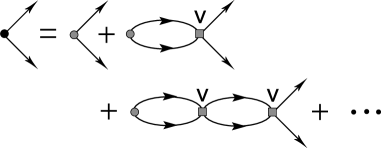
Figure 7: Renormalization of the triplet pair emission (or absorption) amplitude by quantum fluctuations. Vertices come from the singlet $S=0$ scattering channels of two triplets.

We now evaluate the ladder series for scattering processes in Fig. 7, which renormalize $B^{MF}_{\gamma}$ as follows:

$$B^{MF}_{\gamma}\quad\rightarrow\quad B_{\gamma}=B^{MF}_{\gamma}+\Delta B_{\gamma},$$ (44)

where

$$\Delta B_{\gamma} =-\frac{B^{MF}_{\gamma}V^{(S=0)}\Pi_{\gamma}}{1+V^{(S=0)}\Pi_{\gamma}},$$ (45)

and

$$\Pi_{\gamma} =\sum_{\bf k}\int\frac{d\omega}{2\pi i}G^{MF}_{nn}({\bf k},\omega)G^{MF}_{mm}(-{\bf k},-\omega).$$ (46)

In the above $G^{MF}_{nn}$ and $G^{MF}_{mm}$ are the mean-field Green’s function for triplets in the $n$- and $m$-th dimer location in the unit cell. Conventions for the relationship between $\gamma$ and $(n,m)$ are the same as those for $P$ and $Q$ in Eq. (III).

The inclusion of the above quantum fluctuation corrections modifies the triplet Hamiltonian matrix which, after diagonalization, leads to a reduction of the lowest spin gap from $0.795J$ to $0.622J$. Our prediction for the lowest spin gap is still larger than $0.164J$ obtained from exact diagonalization of a 36-site cluster  Sindzingre or $0.08\pm 0.02J$ from a recent 7th order series expansion result (Note that the value from series expansion becomes $0.2J$ in the same finite 36-site cluster) Huse2 . This may suggest that quantum fluctuations beyond what we have considered may be necessary to reach quantitative agreement. At the same time, finite-size effects also need to be examined very carefully.

V Discussion

The Kagome-lattice antiferromagnetic Heisenberg model has been generally regarded as one of the most geometrically frustrated spin systems in two dimension. Because of this, the Kagome lattice has been considered as a promising candidate system for realizing exotic quantum spin liquid ground states. In particular, there are two spin liquid states that have received much attention lately: (i) the U(1) Dirac spin liquid state suggested in a projected wave function study by Ran et al. Ran and (ii) the $Z_{2}$ spin liquid state obtained in a bosonic large-$N$ Sp$(N)$ approach by Sachdev sachdev2 .

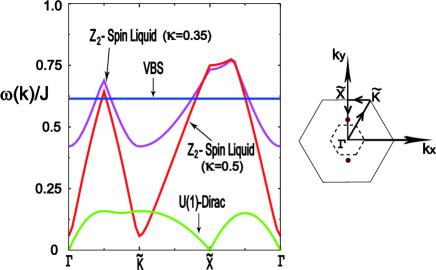
Figure 8: (Color online) Spin-triplet excitation spectra for three candidate ground states of the Kagome-lattice Heisenberg antiferromagnet: (i) the valence bond solid (VBS) with a 36-site unit cell, (ii) the U(1) Dirac spin liquid and (iii) the $Z_{2}$ spin liquid. In the case of the VBS state we plot the renormalized spectrum of the lowest triplet mode including quantum fluctuation effects as described in Sec. IV.4. For these two spin liquid states we plot the lower bound of the two-spinon continuum. The first Brillouin zone for the spin liquid states which has a 3-site triangular unit cell is depicted on the right hand side. The small dotted hexagon shows the first Brillouin zone for the VBS state with a 36-site unit cell. Two red dots lying in the $y$-axis indicate the positions (gauge-dependent) of the Dirac nodes for the U(1) Dirac spin liquid state.

To explicitly compare the lowest spin-triplet excitation energy of the VBS state with those of the above-mentioned spin liquid states, we compute the lower bound of the two-spinon continuum in spin liquid phases. The lower bound (or the bottom of the continuum) is given by

$$\omega({\bf k})=\textrm{Min}_{\bf p}[\epsilon({\bf k}/2+{\bf p}/2)+\epsilon({\bf k}/2-{\bf p}/2)],$$ (47)

where $\epsilon({\bf q})$ is the single spinon excitation energy with momentum ${\bf q}$. An assumption behind this calculation is that spinons themselves are weakly interacting.

For the U(1) Dirac spin liquid state we use the tight-binding spinon Hamiltonian with the mean-field order parameter for spinon hopping $\chi=0.221$ Hastings ; Ran . In the case of the $Z_{2}$ spin liquid state we solve the full saddle point equations for $\kappa=0.35$ and $\kappa=0.5$. Here $\kappa$ is a parameter measuring the strength of quantum fluctuations. In the large-$N$ Sp$(N)$theory the Kagome-lattice system shows magnetic ordering when $\kappa$ is larger than $0.53$ sachdev2 . Results for the lower bound of the two-spinon continuum are plotted in Fig. 8.

Owing to gapless fermionic spinons at nodal points, the U(1)-Dirac spin liquid state exhibits gapless spin-triplet excitations at the zero momentum point, $\Gamma$, and those momenta connecting two Dirac nodes, $\widetilde{X}$. The lower bound of the two-spinon continuum has variations in energy approximately given by $\chi J$. Gapped bosonic spinons of the $Z_{2}$ spin liquid state make the two-spinon spectrum also gapped with relatively large variations for the lower bound. On the other hand, the lowest spin-triplet excitation is completely non-dispersive in our valence bond solid theory. Since the flat dispersion of the lowest spin-triplet excitation is a distinct characteristic of the valence bond solid state, it may be used to distinguish our predictions from those of other spin liquid scenarios.

Acknowledgments

This work was supported by the NSERC, CRC, CIAR, KRF-2005-070-C00044 (YBK) and by the KOSEF through CSCMR SRC (BJY and JY). YBK thanks Brad Marston for careful explanation of his past works and acknowledges the Aspen Center for Physics where some part of this work was initiated. BJY thanks to Choong H. Kim for his valuable comments regarding numerics. Also, two of the authors (BJY, KP) would like to thank Asia Pacific Center for Theoretical Physics (APCTP) for its hospitality.

References

- (1) C. Zeng and V. Elser, Phys. Rev. B 42, 8436 (1990).
- (2) J. B. Marston and C. Zeng, J. Appl. Phys. 69, 5962 (1991).
- (3) S. Sachdev, Phys. Rev. B 45, 12377 (1992).
- (4) R. R. P. Singh and D. A. Huse, Phys. Rev. Lett. 68, 1766 (1992).
- (5) P. W. Leung and V. Elser, Phys. Rev. B 47, 5459 (1993).
- (6) F. Mila, Phys. Rev. Lett. 81, 2356 (1998).
- (7) P. Sindzingre, G. Misguich, C. Lhuillier, B. Bernu, L. Pierre, Ch. Waldtmann and H.-U. Everts , Phys. Rev. Lett. 84, 2953 (2000).
- (8) M. B. Hastings, Phys. Rev. B 63, 014413 (2000).
- (9) P. Nikolic and T. Senthil, Phys. Rev. B 68, 214415 (2003).
- (10) Y. Ran, M. Hermele, P. A. Lee, and X. G. Wen, Phys. Rev. Lett. 98, 117205 (2007).
- (11) R. R. P. Singh and D. A. Huse, Phys. Rev. B 76, 180407(R) (2007).
- (12) R. R. P. Singh and D. A. Huse, arXiv:0801.2735.
- (13) J. S. Helton, K. Matan, M. P. Shores, E. A. Nytko, B. M. Bartlett, Y. Yoshida, Y. Takano, A. Suslov, Y. Qiu, J.-H. Chung, D. G. Nocera, and Y. S. Lee, Phys. Rev. Lett. 98, 107204 (2007).
- (14) P. Mendels, F. Bert, M. A. de Vries, A. Olariu, A. Harrison, F. Duc, J. C. Trombe, J. S. Lord, A. Amato, and C. Baines , Phys. Rev. Lett. 98, 077204 (2007);
- (15) O. Ofer, A. Keren, E. A. Nytko, M. P. Shores, B. M. Bartlett, D. G. Nocera, C. Baines, and A. Amato, cond-mat/0610540.
- (16) T. Imai, E. A. Nytko, B. M. Bartlett, M. P. Shores, and D. G. Nocera, cond-mat/0703141.
- (17) M. A. de Vries, K. V. Kamenev, W. A. Kockelmann, J. Sanchez-Benitez, and A. Harrison, arXiv:0705.0654.
- (18) M. Rigol and R. R. P. Singh, Phys. Rev. B 76, 184403 (2007); G. Misguich and P. Sindzingre, Eur. Phys. J. B 59, 305 (2007).
- (19) Unpublished work by P. Sindzingre and C. Lhuillier as quoted by Singh and Huse Huse2 .
- (20) B. S. Shastry and B. Sutherland, Physica B 108, 1069 (1981).
- (21) S. Sachdev and R. N. Bhatt, Phys. Rev. B 41, 9323 (1990).
- (22) S. Gopalan, T. M. Rice and M. Sigrist, Phys. Rev. B 49, 8901 (1994).
- (23) K. Park and S. Sachdev, Phys. Rev. B 64, 184510 (2001).
- (24) J. P. Blaizot and G. Ripka, Quantum Theory of Finite Systems, (The MIT Press, 1986).
- (25) M. Tinkham, Group Theory and Quantum Mechancies, (McGraw-Hill Book Company, 1964).
- (26) V. N. Kotov, O. Sushkov, Zheng Weihong, and J. Oitmaa, Phys. Rev. Lett. 80, 5790 (1998).
- (27) O. P. Sushkov and V. N. Kotov, Phys. Rev. Lett. 81, 1941 (1998).
- (28) V. N. Kotov, O. P. Sushkov, and R. Eder, Phys. Rev. B. 59, 6266 (1999).
- (29) V. N. Kotov, D. X. Yao, A. H. Castro Neto, and D. K. Campbell, arXiv:0704.0114.