IPMU 08-0011

Gravitational Waves as a Probe of the Gravitino Mass

Fuminobu Takahashi¹, T. T. Yanagida^1,2, and Kazuya Yonekura²

¹ Institute for the Physics and Mathematics of the Universe, University of Tokyo, Chiba 277-8568, Japan
² Department of Physics, University of Tokyo, Tokyo 113-0033, Japan

If gaugino condensations occur in the early universe, domain walls are produced as a result of the spontaneous breaking of a discrete $R$ symmetry. Those domain walls eventually annihilate with one another, producing the gravitational waves. We show that the gravitational waves can be a probe for measuring the gravitino mass, if the constant term in the superpotential is the relevant source of the discrete $R$ symmetry breaking.

1 Introduction

The presence of numerous gauge symmetries is quite a mediocre phenomenon in the string landscape [1] and it is even unlikely that our universe possesses only the standard-model (SM) gauge interactions. Thus, we postulate, through this paper, that we have many (hidden) gauge bosons besides those in the SM.

Each gauge boson is always accompanied by its fermionic partner called a gaugino in supersymmetry (SUSY). Some of the gauginos may condense in the vacuum by the strong forces of the corresponding gauge interactions. Indeed, the gaugino condensation is known to occur in e.g. a $SU(N)$ pure SUSY Yang-Mills theory. In the theory, a continuous $R$ symmetry is explicitly broken to a discrete $Z_{2N}$ subgroup by instantons [2]. The gaugino condensation spontaneously breaks $Z_{2N}$ further down to $Z_{2}$. Accordingly, domain walls are formed at epochs of the condensations in the early universe [3, 4, 5, 6, 7]. If the gaugino condensation occurs before the inflation, the domain walls are diluted away by the subsequent exponential expansion, and there is no cosmological remnant of the walls in the observable universe. However, if the gaugino condensation occurs after the inflation, the domain walls may play an important role in cosmology, since their energy density decreases much more slowly than ordinary matters. In fact, if the domain walls are stable, they will dominate the energy density of the universe in the end, which makes the universe extremely inhomogeneous. To avoid such cosmological disaster, the domain walls must eventually disappear. Fortunately, we know that the discrete $Z_{2N}$ symmetry is not an exact symmetry and hence the domain walls are not stable.

In this paper, we discuss the dynamics of the domain walls formed by the gaugino condensation, assuming that the $SU(N)$ gauge sector does not have sizable couplings to the other sectors. We will briefly discuss the case that such couplings to the SUSY breaking sector are present later. Then the source of the breaking of the $R$ symmetry relevant for the $SU(N)$ sector comes only from the constant term $w_{0}$ in the superpotential $W$. The constant term preserves only the $Z_{2}$ symmetry, and it is needed to cancel the cosmological constant in supergravity (SUGRA). We find that the walls collapse at $H\simeq m_{3/2}$, where $H$ is the expansion rate of the universe and $m_{3/2}$ the gravitino mass. Interestingly, gravitational waves [8] are likely produced during the violent annihilation processes of the domain walls [9]. The typical frequency of the gravitational waves we observe today depends on the gravitino mass, while the intensity is sensitive to the gaugino condensation scale, $\Lambda$. Moreover, thermal history after inflation affects both the frequency and the intensity. We point out in this paper that such stochastic gravitational waves may be detectable by the forthcoming experiments such as Advanced LIGO [10, 11], LCGT [12], LISA [13], BBO [14] and DECIGO [15], for wide ranges of the gravitino mass and the reheating temperature.

2 Gaugino condensation and domain walls

We briefly explain the gaugino condensation and the subsequently formed domain walls. Let us consider a pure $SU(N)$ SUSY Yang-Mills theory . Then the gauge interactions become strong at a dynamical scale $\Lambda$, and the gaugino condensation occurs:

$$\left\langle\lambda^{a}\lambda^{a}\right\rangle_{k}\;=\;-32\pi^{2}e^{2\pi ik/N}\Lambda^{3},$$ (1)

where $k=1,\dots,N$, and there are $N$ degenerate vacua. The effective superpotential below the dynamical scale is given by

$$W_{GC}\;=\;N\Lambda^{3}e^{2\pi ik/N}.$$ (2)

One can derive the forms of the above expressions using the symmetry and the holomorphy of the superpotential.

We assume that the universe undergoes an exponential expansion called inflation. After inflation ends, the inflaton continues to dominate the energy density of the universe until it reheats the universe by the decay. Even before the reheating, there is a background thermal plasma. The maximal temperature of the background plasma can be expressed in terms of the reheating temperature $T_{R}$ and the Hubble parameter during inflation $H_{\rm inf}$ as [16, 17]

$$T_{\rm max}\sim\left(T_{R}^{2}\,H_{\rm inf}M_{P}\right)^{\frac{1}{4}},$$ (3)

where $M_{P}=2.4\times 10^{18}$ GeV is the reduced Planck mass. We require that the maximal temperature of the background plasma is higher than the dynamical scale:

$$T_{\rm max}\;\mathop{}_{\textstyle\sim}^{\textstyle>}\;\Lambda.$$ (4)

Then, the non-zero gaugino condensate is formed after inflation, when the cosmic temperature becomes comparable to $\Lambda$ . When gaugino condensation occurs, one of the $N$ vacua is selected in each domain with the size of $O(\xi)$, where $\xi$ denotes the correlation length, $\xi\sim T^{-1}$. Since the correlation length is much smaller than the horizon scale at the formation, there appear domain walls that connect the distinct vacua populated in each domain. The properties of the domain walls have been extensively studied (see Refs. [6, 18]). In particular, the tension of the wall connecting the adjacent vacua is analytically given by [6]

$$\sigma = 2N\Lambda^{3}\left|e^{2\pi i/N}-1\right|.$$ (5)

In the limit of large $N$, $\sigma$ approaches $4\pi\Lambda^{3}$. In the following analysis we adopt $\sigma=4\pi\Lambda^{3}$ as a reference value.

How does the domain-wall network evolve? The numerical [19, 20, 21] and analytical [22] results obtained so far show that the domain walls reach a scaling regime in simple models. We therefore assume that the evolution of the domain walls is given by the scaling law . That is, an averaged number of the walls per horizon remains the same in the evolution of the universe. This should be the case if the annihilation processes of the domain walls are efficient. The energy density of the domain walls, $\rho_{DW}$, obeying the scaling law is given by

$$\rho_{DW}\;\simeq\;n\,\sigma\,H,$$ (6)

where $H$ is the Hubble parameter, $n$ denotes an averaged number of the walls per horizon, and we expect $n\sim O(1)$. Note that the energy density of the domain walls decreases much more slowly than the radiation and ordinary matters. Therefore, if the domain walls are stable, they come to dominate the energy density of the universe when

$$H\;\sim\;\frac{\sigma}{M_{P}^{2}}.$$ (7)

Once the domain walls dominate the energy density of the universe, the universe will become intolerably inhomogeneous and anisotropic [5]. Therefore the domain walls must disappear before it starts to dominate the universe.

One of the easiest ways to induce the decay of the domain walls is to introduce a bias and lift the degeneracy of the vacua. That is, if the spontaneously broken discrete symmetry is only approximate, the false vacua will decay into the true vacuum in the end, and the domain walls will disappear. Such biased domain walls was first studied by Vilenkin [5]. Here we summarize the result. Let $\epsilon$ denote the bias between the false and true vacua. ($\epsilon$ has mass dimension $4$.) Then the domain walls annihilate with one another and disappear when the tension and the pressure on the wall due to the bias become comparable. The Hubble parameter at the decay is

$$H_{\rm decay}\;\sim\;\frac{\epsilon}{\sigma}.$$ (8)

Since the decay must be complete before the walls come to dominate the universe, there is a lower bound on the bias:

$$\epsilon\;\mathop{}_{\textstyle\sim}^{\textstyle>}\;\frac{\sigma^{2}}{M_{P}^{2}}.$$ (9)

On the other hand, if the bias is too strong, the domain walls are not formed, or even if formed, the walls might disappear before they reach the scaling law. We require that the bias is much smaller than $\rho_{DW}$ when they reach the scaling law soon after the formation. That is,

$$\sigma H_{f}\;\gg\;\epsilon$$ (10)

with

$$H_{f}\;\sim\;\left\{\begin{array}[]{cc}\displaystyle{\frac{\Lambda^{2}}{M_{P}}}&{\rm~~~for~~}T_{R}>\Lambda\\ \displaystyle{\frac{\Lambda^{4}}{T_{R}^{2}M_{P}}}&{\rm~~~for~~}T_{R}<\Lambda\end{array},\right.$$ (11)

where $H_{f}$ denotes the Hubble parameter at the domain-wall formation.

Our concern here is if such a bias exists in the case of the gaugino condensation. Fortunately, there is indeed a source for the explicit breaking of the discrete $Z_{2N}$ symmetry. In order to cancel the cosmological constant, we need to introduce a constant $w_{0}$ in the superpotential. The constant explicitly breaks $Z_{2N}$ down to $Z_{2}$, and so, the degeneracy of the vacua is lifted. To see this, we write down the scalar potential in SUGRA using the effective superpotential $W=W_{GC}+w_{0}$ ,

$$V\;\simeq\;-3N\frac{w_{0}^{*}}{M_{P}^{2}}\Lambda^{3}e^{2\pi ik/N}+{\rm h.c.}.$$ (12)

Thus, depending on the relative phase between the gaugino condensate and $w_{0}$, the scalar potentials take different values in the distinct $N$ vacua. The typical size of the bias between the adjacent vacua is given by

$$\epsilon\;\simeq\;\alpha\,m_{3/2}\Lambda^{3},$$ (13)

where we have used $|w_{0}|=m_{3/2}M_{P}^{2}$, and $\alpha=O(10)$ is a numerical coefficient. Throughout this paper, we assume that $w_{0}$ is the dominant source of the bias. Substituting (5) and (13) into (8), one can see that the Hubble parameter at the decay is given by

$$H_{\rm decay}\;\sim\;m_{3/2}.$$ (14)

Thus, as long as the constant $w_{0}$ is the main source of the bias, the timing of the domain-wall decay is determined by the gravitino mass. The constraints on the bias, (9) and (10), read

$$\Lambda_{\rm min}^{3}\;\ll\;\Lambda^{3}\;\mathop{}_{\textstyle\sim}^{\textstyle<}\;0.1\,m_{3/2}M_{P}^{2}$$ (15)

with

$$\Lambda_{\rm min}\;\equiv\;\left\{\begin{array}[]{cc}\displaystyle{\sqrt{m_{3/2}M_{P}}}&{\rm~~~for~~}T_{R}>\Lambda\\ \displaystyle{\left(m_{3/2}M_{P}T_{R}^{2}\right)^{\frac{1}{4}}}&{\rm~~~for~~}T_{R}<\Lambda\end{array}\right..$$ (16)

As we see in the next section, the intensity of the gravitational waves increases as $\Lambda$ becomes large. When $\Lambda$ takes the largest allowed value, the energy of the domain walls becomes comparable to the total energy of the universe at the decay.

The energy density stored in the domain walls must go into light degrees of freedom. In this paper we simply assume that the energy quickly goes into another hidden massless $U(1)$ gauge bosons through loop diagrams of some heavy vector-like quarks charged under both gauge symmetries . Since we assume that the domain walls decay before they come to dominate the universe, the energy of the hidden radiation is subdominant compared to the visible one. In Sec. 4, we will discuss a possibility to observe the effect of the hidden radiation. Even if the domain walls decay into the visible particles, the following arguments on the gravitational waves remain intact, as long as the decay proceeds fast enough.

Lastly let us summarize our picture. The domain walls are formed when the gauginos condense, i.e., $T\sim\Lambda$. Those walls evolve according to the scaling law (6) until $H\sim m_{3/2}$. When $H\sim m_{3/2}$, the domain walls experience the pressure due to the bias, and they are pulled toward one another. After violent collisions of the domain walls, the false vacua decay into the true vacuum, and the domain walls disappear. The energy stored inside the domain walls and the false vacua will be released into light degrees of freedom. Most importantly, since the walls are spatially extended two dimensional objects, the collisions likely occur in such a way widely deviated from the spherical symmetry, leading to the production of the gravitational waves. Thus the domain walls of the gaugino condensate may have left their traces in the gravitational waves, which will be discussed in the next section.

3 Gravitational waves

We discuss here the properties of the gravitational waves produced from the decay of the domain walls. To detect the gravitational waves by the forthcoming experiments, the frequency and the intensity must be in certain ranges.

Let us first consider the frequency of the gravitational waves. The gravitational waves are expected to peak at the frequency corresponding to a typical physical scale when they are produced. In our case, this frequency corresponds to the horizon scale at the decay, i.e., $f_{*}\sim m_{3/2}$. The frequency is red-shifted due to the subsequent cosmic expansion, and the frequency we observe today, $f_{0}$, is much smaller than $f_{*}$:

$$f_{0}\;=\;\frac{a_{*}}{a_{0}}\,f_{*},$$ (17)

where $a_{0}$ and $a_{*}$ are the scale factors at present and at the formation of the gravitational waves, respectively. The amount of the red-shift, or equivalently, $a_{*}/a_{0}$, depends on the thermal history of the universe.

If the reheating of the universe is completed before $H\sim m_{3/2}$, the universe is radiation-dominated afterwards until the matter-radiation equality. The ratio of the scale factors is estimated by

$$\frac{a_{*}}{a_{0}}\;\simeq\;6\times 10^{-14}\left(\frac{g_{*}}{200}\right)^{-\frac{1}{3}}\left(\frac{T_{*}}{1{\rm\,GeV}}\right)^{-1},$$ (18)

where $T_{*}$ denotes the cosmic temperature, and $g_{*}$ counts the relativistic degrees of freedom, both evaluated at $a=a_{*}$. Thus the frequency at present, $f_{0}$, is directly related to the gravitino mass as

$$f_{0} \simeq 0.1\,{\rm Hz}\,\left(\frac{g_{*}}{200}\right)^{-\frac{1}{12}}\left(\frac{m_{3/2}}{1{\rm\,keV}}\right)^{\frac{1}{2}}.$$ (19)

On the other hand, if the reheating is not completed when $H\sim m_{3/2}$, the universe is matter-dominated until the reheating. Then the amount of the red-shift is modified as

$$\frac{a_{*}}{a_{0}}\;\simeq\;1\times 10^{-21}\left(\frac{T_{R}}{1{\rm\,GeV}}\right)^{\frac{1}{3}}\left(\frac{m_{3/2}}{1{\rm\,keV}}\right)^{-\frac{2}{3}}.$$ (20)

The present frequency becomes

$$f_{0}\;\simeq\;2\,{\rm mHz}\,\left(\frac{T_{R}}{1{\rm\,GeV}}\right)^{\frac{1}{3}}\left(\frac{m_{3/2}}{1{\rm\,keV}}\right)^{\frac{1}{3}}.$$ (21)

Surprisingly, the peak frequencies of the gravitational waves coincide with those covered by various ongoing and planned experiments, for wide ranges of the gravitino mass and the reheating temperature. We will come to this point later.

The intensity of the gravitational waves decreases as the universe expands, since the amplitude is red-shifted for a mode with the wavelength less than the horizon size. In order to characterize the intensity, one may use a dimensionless quantity $\Omega_{\rm gw}(f)$ defined by

$$\Omega_{\rm gw}(f)\;\equiv\;\frac{1}{\rho_{c}}\frac{d\rho_{gw}}{d\log f},$$ (22)

where $\rho_{gw}$ is the energy density of the gravitational waves, $\rho_{c}$ the critical energy density, and $f$ the frequency.

Let us estimate the magnitude of $\Omega_{\rm gw}(f)$ (see [8]). The energy of the gravitational waves in a horizon at $H=m_{3/2}$ is estimated by

$$E_{gw}\;\sim\;G\,\frac{M_{DW}^{2}}{R_{*}}\sim\frac{2\pi\Lambda^{6}}{m_{3/2}^{3}M_{P}^{2}},$$ (23)

where $G=1/(8\pi M_{P}^{2})$ is the Newton constant, $M_{DW}$ the energy stored in the domain walls, and $R_{*}$ the typical spatial scale of the energy distribution. In the second equality in (23), we have used $M_{DW}\sim\sigma/m_{3/2}^{2}$ and $R_{*}\sim 1/m_{3/2}$. If the reheating is completed before $H=m_{3/2}$, we have

$$\Omega_{\rm gw}(f_{0})h^{2} \sim 10^{-7}\left(\frac{g_{*}}{200}\right)^{-\frac{1}{3}}\left(\frac{\Lambda^{3}}{0.1\,m_{3/2}M_{P}^{2}}\right)^{2},$$ (24)

where $f_{0}$ is given by (19), and $h$ is the present Hubble parameter in units of $100$ km/s/Mpc. For $\Lambda$ close to its upper bound given by (15), therefore, the energy density of the gravitational wave amounts to one percent of the cosmic microwave background photons! If the reheating is not completed at $H=m_{3/2}$, the gravitational waves are diluted by the entropy production of the inflaton. The density parameter, $\Omega_{\rm gw}$, is then given by

$$\Omega_{\rm gw}(f_{0})h^{2}\;\sim\;10^{-12}\left(\frac{T_{R}}{100{\rm\,GeV}}\right)^{\frac{4}{3}}\left(\frac{m_{3/2}}{1{\rm\,keV}}\right)^{-\frac{2}{3}}\left(\frac{\Lambda^{3}}{0.1m_{3/2}M_{P}^{2}}\right)^{2},$$ (25)

where $f_{0}$ is given by (21). Note that the intensity of the gravitational waves is very sensitive to the dynamical scale, $\Lambda$. In order to detect the gravitational waves from the domain-wall decay, $\Lambda$ must be close to its upper bound.

We have made a rough estimate of the intensity of the gravitational waves in the above. Further detailed analyses on the domain-wall dynamics may reveal the presence of additional suppression factors. However, there are at least two reasons to believe that the gravitational waves produced by the domain-wall dynamics are not extremely suppressed. One is that the collisions among the domain walls are strongly first order phase transition, since they are decoupled from the thermal bath. The other is that the domain-walls are spatially extended two dimensional objects, which exhibits a peculiar dependence on the spatial scale. To see this more explicitly, let us consider the dependence of $\Omega_{\rm gw}$ on the spatial scale, $R$. Using $M_{DW}\propto R^{2}$, we have $E_{gw}\propto R^{3}$, leading to $\Omega_{\rm gw}\propto R^{0}$! This is very different from the ordinary non-relativistic matters, which would lead to $\Omega_{\rm gw}\propto R^{2}$. Therefore, the resultant intensity of the gravitational waves is independent of the spatial scale, which makes the above rough estimate more robust . Thus, the domain-wall dynamics may be an ideal source for generating the gravitational waves in the early universe.

Here let us briefly mention the sensitivities of the ongoing and planned experiments on the gravitational waves. One of the ground-based experiments, LIGO [24], is in operation and it is sensitive to the frequency between $O(10)$ Hz and $10^{4}$ Hz. The latest upper bound is $\Omega_{\rm gw}h^{2}<6.5\times 10^{-5}$ around $100$ Hz [25], and an upgrade of the experiment, Advanced LIGO, would reach sensitivities of $O(10^{-9})$. The sensitivity of LCGT would be more or less similar to that of Advanced LIGO. There are also planned space-borne interferometers such as LISA, BBO and DECIGO. LISA is sensitive to the band of $(0.03-0.1)\,{\rm mHz}\mathop{}_{\textstyle\sim}^{\textstyle<}f_{0}\mathop{}_{\textstyle\sim}^{\textstyle<}0.1$ Hz, and it can reach $\Omega_{\rm gw}h^{2}<10^{-12}$ at $f_{0}=1$ mHz. Moreover, BBO and DECIGO will cover $10{\rm\,mHz}\mathop{}_{\textstyle\sim}^{\textstyle<}f_{0}\mathop{}_{\textstyle\sim}^{\textstyle<}10^{2}$ Hz with much better sensitivity.

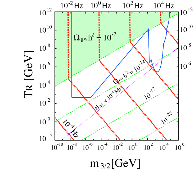
In Fig. 1, we show the contours of the frequencies: $f_{0}=10^{-4}$, $10^{-2}$, $1$, $10^{2}$, and $10^{4}$ Hz, and the (maximal) intensities: $\Omega_{\rm gw}h^{2}=10^{-22},10^{-17},10^{-12}$ and $10^{-7}$, in the parameter space of the gravitino mass and the reheating temperature. Here we have set $\Lambda$ to be the largest value allowed by (15). In the shaded triangle region, $\Omega_{\rm gw}h^{2}$ is saturated to $10^{-7}$, since the reheating is complete before the domain-wall decay (see (19) and (24)). Also we schematically show the upper bounds on $T_{R}$ from the gravitino problem [26, 27, 28, 29, 30, 31, 32, 33, 34] (solid (blue) line). The dotted (purple) line shows the constraint obtained by (4) and $H_{\rm inf}<10^{-4}\,M_{P}$ [35], and the region below the line is excluded .

One can see that, for wide ranges of $m_{3/2}$ and $T_{R}$, the peak frequencies of the gravitational waves correspond to those covered by the ongoing and planned experiments. Compared with the sensitivities of the experiments mentioned above, the gravitational waves from the domain-wall decay may be detectable, even by Advanced LIGO. Once it is detected, we will be able to obtain information on both the gravitino mass and the reheating temperature. In particular, for $m_{3/2}\mathop{}_{\textstyle\sim}^{\textstyle<}O(10)$ eV, the measured frequency can be directly related to the gravitino mass by (19).

Figure 1: Contours of the frequency (thick-dotted, red) and the maximal intensity (thin-dashed, green) of the gravitational waves from the domain-wall decay. $\Lambda$ is set to be the largest value allowed by (15). The solid (blue) line schematically shows upper bounds on the reheating temperature from the gravitino problem. The dotted (purple) line shows the bound coming from (4) and $H_{\rm inf}<10^{-4}\,M_{P}$, and the region below the dotted (purple) line is excluded. Note that the bound is not applied if the $SU(N)$ gauginos are not in thermal equilibrium. LIGO and LISA are sensitive to the bands of $O(10){\rm\,Hz}\mathop{}_{\textstyle\sim}^{\textstyle<}f_{0}\mathop{}_{\textstyle\sim}^{\textstyle<}10^{4}$ Hz and $0.1{\rm\,mHz}\mathop{}_{\textstyle\sim}^{\textstyle<}f_{0}\mathop{}_{\textstyle\sim}^{\textstyle<}0.1$ Hz, respectively, while BBO and DECIGO will cover $10{\rm\,mHz}\mathop{}_{\textstyle\sim}^{\textstyle<}f_{0}\mathop{}_{\textstyle\sim}^{\textstyle<}10^{2}$ Hz with much better sensitivity.

4 Discussion and conclusions

We have so far focused on the gravitational waves produced by the domain-wall dynamics. Let us here briefly discuss the decay products of the domain walls. After the collisions of the domain walls, the energy stored in the walls is assumed to decay into the hidden massless $U(1)$ gauge bosons. Then there is a relation between the energies of the hidden radiation and the gravitational waves:

$$\Omega_{hid}\sim 2\left(\frac{m_{3/2}M_{P}^{2}}{\Lambda^{3}}\right)\,\Omega_{\rm gw},$$ (26)

where $\Omega_{hid}$ is the density parameter of the hidden radiation. Therefore, the hidden radiation is always more abundant than the gravitational waves (see (15)). For the largest allowed value of $\Lambda$, we have $\Omega_{hid}\sim 20\,\Omega_{\rm gw}$. It might be possible to measure $\Omega_{hid}$ indirectly by using the big bang nucleosynthesis (BBN), the cosmic microwave background, and large-scale structure data. Indeed, measurements of the light-element abundances give $\Omega_{hid}h^{2}\mathop{}_{\textstyle\sim}^{\textstyle<}1.5\times 10^{-5}$ at 95% C.L. [36], which is translated to the bound on the gravitational waves,

$$\Omega_{\rm gw}h^{2}\;\mathop{}_{\textstyle\sim}^{\textstyle<}\;8\times 10^{-6}\frac{\Lambda^{3}}{m_{3/2}M_{P}^{2}}.$$ (27)

Therefore, if the domain walls mainly decay into the hidden massless $U(1)$ gauge bosons, the indirect measurement of $\Omega_{hid}$ can set a bound on $\Omega_{\rm gw}$ .

If SUSY is realized at a scale much higher than the weak scale, it may be difficult to directly produce SUSY particles in the accelerator experiments like LHC or ILC. Then, it will be interesting if we can probe high-energy physics inaccessible to the accelerator experiments, by observing the gravitational waves. For $m_{3/2}\sim 10^{4}-10^{6}$ GeV, the frequency of the gravitational waves is in the band of $10^{2}{\rm\,Hz}\mathop{}_{\textstyle\sim}^{\textstyle<}f_{0}\mathop{}_{\textstyle\sim}^{\textstyle<}10^{4}$ Hz, where the ground-based experiments are sensitive (see Fig. 1). If the gravitino mass is heavier than $10^{6}$ GeV, however, $f_{0}$ exceeds the frequencies to which the ongoing and planned experiments are sensitive. Even in this case, one may be able to indirectly observe the hidden radiation related to the gravitational waves by (26).

We have assumed that the constant in the superpotential, $w_{0}$, is the relevant source of the discrete $R$ symmetry breaking. If the $SU(N)$ gauge sector has couplings to the SUSY breaking sector, the gaugino mass $m_{\lambda}$ generically receives contribution larger than the anomaly mediation. In that case the relation between $f_{0}$ and $m_{3/2}$ will be lost. However, the properties of the gravitational waves we have derived in the previous section are still valid if one replaces the gravitino mass by the $(16\pi^{2}/3Ng^{2})m_{\lambda}$.

Gaugino condensation is ubiquitous, if there are many gauge groups besides the SM ones in nature. The domain walls are generically formed when the gauginos condense. To avoid cosmological disaster, however, those domain walls must disappear. Since the discrete $R$ symmetry is explicitly broken by the constant term $w_{0}$ in the superpotential, the domain walls are unstable and eventually decay into light particles. Interestingly, the gravitational waves are generated at the domain-wall collisions, and they contain valuable information on high-energy physics and the early universe. In this paper we have pointed out that the resultant gravitational waves can be a probe for measuring the gravitino mass, if $w_{0}$ is the relevant source of the discrete $R$ symmetry breaking.

References

- [1] L. Susskind, arXiv:hep-th/0302219.
- [2] E. Witten, Nucl. Phys. B 202, 253 (1982).
- [3] Y. B. Zeldovich, I. Y. Kobzarev and L. B. Okun, Zh. Eksp. Teor. Fiz. 67, 3 (1974) [Sov. Phys. JETP 40, 1 (1974)].
- [4] T. W. B. Kibble, J. Phys. A 9, 1387 (1976).
- [5] A. Vilenkin, Phys. Rev. D 23 (1981) 852.
- [6] G. R. Dvali and M. A. Shifman, Phys. Lett. B 396, 64 (1997) [Erratum-ibid. B 407, 452 (1997)].
- [7] T. Matsuda, Phys. Lett. B 436, 264 (1998).
- [8] See M. Maggiore, Phys. Rept. 331, 283 (2000), for a review.
- [9] M. Gleiser and R. Roberts, Phys. Rev. Lett. 81, 5497 (1998).
- [10] B. C. Barish and R. Weiss, Phys. Today 52N10 (1999) 44.
- [11] P. Fritschel, arXiv:gr-qc/0308090.
- [12] K. Kuroda et al., Class. Quant. Grav. 19, 1237 (2002).
- [13] LISA Pre-Phase A Report, 2nd Ed. (1998): http://www.srl.caltech.edu/lisa/documents/PrePhaseA.pdf
- [14] J. Crowder and N. J. Cornish, Phys. Rev. D 72, 083005 (2005).
- [15] N. Seto, S. Kawamura and T. Nakamura, Phys. Rev. Lett. 87, 221103 (2001).
- [16] T. Asaka and M. Kawasaki, Phys. Rev. D 60, 123509 (1999).
- [17] G. F. Giudice, E. W. Kolb and A. Riotto, Phys. Rev. D 64, 023508 (2001).
- [18] A. Kovner, M. A. Shifman and A. Smilga, Phys. Rev. D 56, 7978 (1997).
- [19] W. H. Press, B. S. Ryden and D. N. Spergel, Ap. J. 347, 590 (1989).
- [20] D. Coulson, Z. Lalak and B. A. Ovrut, Phys. Rev. D 53, 4237 (1996).
- [21] S. E. Larsson, S. Sarkar and P. L. White, Phys. Rev. D 55, 5129 (1997).
- [22] M. Hindmarsh, Phys. Rev. Lett. 77, 4495 (1996).
-
[23]
L. Randall and R. Sundrum,
Nucl. Phys. B 557, 79 (1999);
G. F. Giudice, M. A. Luty, H. Murayama and R. Rattazzi, JHEP 9812, 027 (1998);
J. A. Bagger, T. Moroi and E. Poppitz, JHEP 0004, 009 (2000). - [24] A. Abramovici et al., Science 256 (1992) 325.
- [25] Abbott, B. et al. (The LIGO Scientific Collaboration) Astrophys. J. 659, 918 (2007).
- [26] M. Kawasaki, K. Kohri and T. Moroi, Phys. Lett. B 625, 7 (2005); Phys. Rev. D 71, 083502 (2005).
- [27] K. Kohri, T. Moroi and A. Yotsuyanagi, Phys. Rev. D 73, 123511 (2006).
- [28] K. Jedamzik, Phys. Rev. D 74, 103509 (2006).
- [29] T. Moroi, H. Murayama and M. Yamaguchi, Phys. Lett. B 303, 289 (1993).
- [30] M. Bolz, W. Buchmuller and M. Plumacher, Phys. Lett. B 443, 209 (1998).
- [31] M. Bolz, A. Brandenburg and W. Buchmuller, Nucl. Phys. B 606, 518 (2001).
- [32] J. R. Ellis, K. A. Olive, Y. Santoso and V. C. Spanos, Phys. Lett. B 588, 7 (2004); L. Roszkowski, R. Ruiz de Austri and K. Y. Choi, JHEP 0508, 080 (2005); D. G. Cerdeno, K. Y. Choi, K. Jedamzik, L. Roszkowski and R. Ruiz de Austri, JCAP 0606, 005 (2006).
- [33] F. D. Steffen, JCAP 0609, 001 (2006).
- [34] J. Pradler and F. D. Steffen, Phys. Rev. D 75, 023509 (2007); Phys. Lett. B 648, 224 (2007).
- [35] D. N. Spergel et al. [WMAP Collaboration], Astrophys. J. Suppl. 170, 377 (2007).
- [36] G. Mangano, A. Melchiorri, O. Mena, G. Miele and A. Slosar, JCAP 0703, 006 (2007).