Lepton flavor violation in predictive supersymmetric GUT models
)
Abstract
There have been many theoretical models constructed which aim to explain the neutrino masses and mixing patterns. While many of the models will be eliminated once more accurate determinations of the mixing parameters, especially , are obtained, charged lepton flavor violation experiments are able to differentiate even further among the models. In this paper, we investigate various rare lepton flavor violation processes, such as and conversion, in five predictive supersymmetric (SUSY) models and their allowed soft-SUSY breaking parameter space in the constrained minimal SUSY standard model. Utilizing the Wilkinson Microwave Anisotropy Probe dark matter constraints, we obtain lower bounds on the branching ratios of these rare processes and find that at least three of the five models we consider give rise to predictions for that will be tested by the MEG Collaboration at PSI. In addition, the next generation conversion experiment has sensitivity to the predictions of all five models, making it an even more robust way to test these models. While generic studies have emphasized the dependence of the branching ratios of these rare processes on the reactor neutrino angle, , and the mass of the heaviest right-handed neutrino, , we find very massive is more significant than large in leading to branching ratios near to the present upper limits.
pacs:
14.60.Pq, 12.10.Dm, 12.15.FfI Introduction
The recent compilation of oscillation data from the atmospheric atm , reactor reactor , and long baseline lbl neutrino experiments has provided solid evidence that neutrinos have small but non-zero masses. A global fit to current data gives the following limits for the mixing parameters Maltoni:2004ei ,
| (1) | |||||
| (2) | |||||
| (3) |
Since then, the measurements of neutrino oscillation parameters have entered a precision era. On the other hand, as no information exists for the value of , the Dirac or Majorana nature of the neutrinos, the Dirac and/or Majorana CP phases, and the neutrino mass hierarchy, there are discoveries that are still yet to come.
In the Standard Model (SM), due to the lack of right-handed neutrinos and the conservation of lepton numbers, neutrinos are massless. To generate non-zero neutrino masses thus calls for physics beyond the SM. There have been many theoretical ideas proposed with an attempt to accommodate the experimentally observed small neutrino masses and the larger mixing angles among them. In Ref. Albright:2006cw , we have surveyed 63 models in the literature that are still viable candidates and have reasonably well-defined predictions for . We found that the predictions for of half of the models cover the range from 0.015 to the present upper bound of 0.13. Consequently, half of the models can be eliminated in the next generation of reactor experiments.
One of the implications of the observation of neutrino oscillation is the possibility of measurable branching ratio for charged lepton flavor-violating (LFV) decays. While not the case in the SM, predictions of the supersymmetric (SUSY) Grand Unified Theories (GUT) for these rare decays are much enhanced, as these processes are suppressed by the SUSY scale, rather than the Plank scale BorzMas . Furthermore, as different models obtain large neutrino mixing angles through different mechanisms, their predictions for the LFV charged lepton decays can be very distinct. Consequently, LFV charged lepton decays may provide a way to distinguish different SUSY GUT models.
Among the models aiming to explain the neutrino masses and mixing, a particularly promising class are those based on (SUSY) SO(10); for recent reviews of SO(10) models, see Chen:2003zv . In this paper, we investigate the predictions for various LFV charged lepton decays as well as muon-electron conversion in five of the SUSY SO(10) models, assuming constrained minimal SUSY standard model (CMSSM) boundary conditions where only five soft-SUSY breaking parameters are present. Furthermore, we impose the Wilkinson Microwave Anisotropy Probe (WMAP) dark matter constraints in the neutralino, stau and stop coannihilation regions. Specifically, we present the allowed values for these soft-SUSY parameters for various branching ratios of these rare LFV processes. In addition, the lower bounds on the predictions for these rare processes in the five different SUSY SO(10) models are given. We find that the predictions in these models are very distinct. We note the crucial role of the WMAP constraints in deducing the lower bounds on the predictions.
Many authors have previously studied the branching ratio predictions for charged LFV decays in the SUSY GUT framework. Rather than study specific models, they generally adopt a generic approach and assume a nearly diagonal Cabibbo-Kobayashi-Maskawa (CKM)-like or bimaximal Pontecorvo-Maki-Nakagawa-Sakata (PMNS)-like mixing matrix to diagonalize the Yukawa neutrino matrix generic . Following the procedure of Casas and Ibarra CasasIbarra to invert the seesaw formula, they have carried out Monte Carlo studies by scanning the unknown right-handed neutrino mass spectrum and the angles and phases of the inversion matrix in order to present scatter plots of the rare branching ratios. A few exceptions to this procedure can be found in Ref. exceptions . Here we are interested in specific models in order to determine the ability of the LFV experiments to differentiate among and rule out some models. The models chosen are highly predictive and illustrate a wide variety of textures for the charged lepton and neutrino mass matrices, and predictions for the right-handed neutrino mass spectrum and the reactor neutrino mixing angle, .
In Sec. II we describe the five representative SUSY SO(10) models that we have analyzed. In Sec. III we review LFV charged lepton decays in the SM and SUSY GUTs and present the predictions for the five SUSY SO(10) models considered. In Sec. IV their expectations for conversion are given. Sect. V concludes this paper.
II PREDICTIVE SUPERSYMMETRIC GRAND UNIFIED MODELS CONSIDERED
We begin with a brief discussion of the general formalism on which the supersymmetric grand unified models are based. For all five models to be illustrated, the seesaw mechanism seesaw is of the conventional type I leading to normal hierarchies for the light Majorana neutrinos. The leptonic sector of the Yukawa superpotential at the GUT scale can then be written as
| (4) |
where represents the left-handed lepton doublet, the
left-handed conjugate neutrino singlet, and the left-handed conjugate
charged lepton of one of the three dimensional representations of
. When the two Higgs doublets, and , acquire vacuum
expectation values, the charged lepton and neutrino mass matrices are
generated and can be written in form
| (5) |
With the entries in much larger than those in , the light Majorana neutrino mass matrix is given by the well-known type I seesaw formula seesaw ,
| (6) |
Note that the above Dirac mass matrix entries, and , are written in right - left order and appear in the flavor basis. As such, the matrices can be diagonalized by the unitary transformations
| (7) |
by forming the Hermitian products, calculating the left and right unitary transformations of column eigenvectors, and phase rotating the complex symmetric and matrices, so their mass eigenvalues are real. The PMNS neutrino mixing matrix PMNS is then given by .
On the other hand for later use, it is convenient to transform to the bases where and are diagonal and denoted by primed quantities. In this case
| (8) |
where now , since is just the identity matrix. A comparison of the seesaw diagonalization matrices then reveals that the transformed Dirac neutrino matrix in the new basis is given by
| (9) |
in terms of the original matrix in the flavor bases.
With either basis, the left-handed neutrino PMNS mixing matrix can be written as , where by convention PDB
| (10) |
in terms of the three mixing angles, and ; and the Dirac phase, , in analogy with the quark mixing matrix. The Majorana phase matrix,
| (11) |
written in terms of the two Majorana phases, and , is required since an arbitrary phase transformation is not possible when one demands real diagonal neutrino mass entries in the transformation of in Eq. (7) or in Eq. (8).
With this background in mind, we now turn to a brief discussion of the five models we have considered for our lepton flavor violation study. The grand unification symmetry is an economical and attractive one Chen:2003zv , for all sixteen left-handed quark and lepton fields and their left-handed conjugates fit neatly into one representation per family. Many models exist in the literature which differ from one another by their Higgs representation assignments and type of flavor symmetry imposed, if any. To appreciate this, it is of interest to note the following decompositions of the direct product of representations:
| (12) |
where in the first product the and matrices are symmetric, while the is antisymmetric under the interchange of family indices.
Given this group structure for , there are two general classes of models which have been extensively studied. Those with Higgs in the , and possibly the and/or , dimensional representations are often referred to as the minimal Higgs models minimal and lead to symmetric or antisymmetric matrix elements, or a superposition of the two. The advantage is that the couplings are renormalizable and preserve R-parity, but the latter representations are of rather high rank and disfavored in the string theory framework. The other class typically involves the lower rank Higgs representations such as , with some non-renormalizable effective operators formed from them, lopsided but R-parity is not conserved. They can lead to lopsided mass matrices for the charged lepton and down quark mass matrices, due to the structure present in the ’s. As such, one may anticipate that they will predict a higher level of lepton flavor violation than the first class. The triplet components in the Higgs representations in all five models considered have no electroweak VEV and hence lead to the conventional type I seesaw mechanism with the prediction of normal hierarchy for the light left-handed neutrino spectrum normal . We elaborate on each model in turn but give only the neutrino and charged lepton mass matrices. All successfully predict the observed quark structure and CKM mixings.
II.1 Albright - Barr Model
This model, based on with a flavor symmetry ABmodel , is of the lopsided variety and has matrices of the following textures:
| (13) |
where the parameters have the values . The right-handed Majorana mass matrix is given by
| (14) |
where GeV. One finds
| (15) |
A value of assures that and that the corresponding lopsided nature of the 23 element of the down quark mass matrix gives a good fit to the results for the quark sector. The elements of the Dirac neutrino matrix were added Amodel to the original model to give a better fit to baryogenesis arising from resonant leptogenesis involving the two lighter right-handed neutrinos leptogen . Evolution downward from the GUT scale to has little effect on the mixing angles due to the small , the opposite CP-parity of the lighter two right-handed Majorana neutrinos, and their large hierarchy with the heaviest one; but serves to lower the values of the ’s and and relative to their GUT scale values.
II.2 Chen - Mahanthappa Model
This model, based on with a flavor symmetry CMmodel , is of the minimal Higgs variety leading to symmetric entries in the mass matrices:
| (16) |
where GeV and the parameters have the values . The solar and atmospheric neutrino mass squared differences, and were used as input to determine the and parameters in the effective light left-handed Majorana neutrino mass matrix
| (17) |
One then finds
| (18) |
For this model, a value of is used. The effect of evolution from the GUT scale to is to raise and to lower .
II.3 Cai - Yu Model
This model is based on with an flavor symmetry CYmodel . The Higgs fields appear in six ’s, three ’s, three , and one representations of , distinguished by their flavor assignments. Of the 14 pairs of Higgs doublets at the GUT scale, all but one pair are assumed to get superheavy. The charged lepton mass matrix is chosen to be diagonal, while the right-handed Majorana neutrino mass matrix is proportional to the identity matrix, so all three heavy neutrinos are degenerate. The Dirac neutrino and charged lepton mass matrices are symmetric and given by
| (19) |
where the parameters have the values , all in GeV. The common mass of the degenerate right-handed neutrinos is determined to be GeV, so as to fit with the aid of the seesaw formula. The authors find
| (20) |
A value of is used to evolve the quark and charged lepton masses, though the neutrino masses and mixings have not been evolved downward to the electroweak scale.
II.4 Dermisek - Raby Model
This model is based on with a family symmetry DRmodel . The charged lepton and down quark mass matrices have lopsided textures, but they are not so extreme as in the case of the Albright - Barr model:
| (21) |
where GeV and the parameters have the values . The right-handed Majorana mass matrix is diagonal with mass eigenvalues , , GeV. These parameters were chosen by making use of the central experimental values for and at the time of writing. The authors find
| (22) |
The evolution has been carried out with and GeV down to and then down to the 1 GeV scale for the light neutrino masses.
II.5 Grimus - Kuhbock Model
This model is based on with an flavor symmetry GKmodel . The Higgs fields appear in one each of the , , and dimensional representations of . The fermion mass matrices are generated by renormalizable Yukawa couplings of these Higgs fields to the three families placed in ’s. The Dirac neutrino and charged lepton mass matrices are written as linear combinations of the Yukawa couplings of the , , and Higgs representations, respectively, while the right-handed Majorana matrix is proportional only to the latter:
| (23) |
where the individual Higgs contributions to the mass matrices are given by
| (24) |
in the right-left order we have adopted. The coefficient parameters are taken to be . A value of is used to evolve the quark and charged lepton masses downward to the electroweak scale. One finds then that
| (25) |
Although the results are impressive, the authors do note that 21 parameters have been introduced in order to obtain the results. Hence the model should be viewed as an existence proof that the lepton masses and mixings as well as the quark masses and mixings can be described in the framework of renormalizable couplings with only the three Higgs representations contributing to the Yukawa couplings.
| Models | Higgs Content | Flavor Symmetry | (GeV) | Interesting Features | ||
|---|---|---|---|---|---|---|
| AB | 5 | 0.0020 | Large hierarchy with lightest | |||
| () | two nearly degenerate leads to | |||||
| resonant leptogenesis. | ||||||
| CM | 10 | 0.013 | Large hierarchy with heaviest | |||
| () | more than 3 orders of magnitude | |||||
| below GUT scale; large . | ||||||
| CY | 10 | 0.0029 | Degenerate spectrum 4 orders | |||
| () | of magnitude below GUT scale. | |||||
| DR | 50 | 0.0024 | Mild hierarchy almost 3 orders | |||
| () | of magnitude below GUT scale. | |||||
| GK | 10 | 0.00059 | Mild hierarchy just 1 order of | |||
| () | magnitude below GUT scale; | |||||
| rather small . |
We close this section by summarizing the features of these models in Table I. Three of the models have similar predictions for , near the expected reach of the Double CHOOZ and Daya Bay reactor experiments newreactors . One of the models predicts a value near the present upper limit placed by the CHOOZ experiment CHOOZ , while the fifth model predicts a value of which is essentially beyond reach until a Neutrino Factory becomes a reality. We shall see what potential success charged lepton flavor violation experiments will have in further distinguishing the viable models.
III LEPTON FLAVOR VIOLATION IN RADIATIVE DECAYS
We now turn to the subject of charged lepton flavor violation that can occur in the radiative decays, , , and . In the SM with the addition of three massive right-handed neutrinos, we observe that the individual lepton numbers, and , are not individually conserved. In radiative lepton decays, the flavor violation arises in one loop, where the neutrino insertion involves lepton flavor-changing Yukawa couplings of the left-handed and right-handed neutrinos; cf. Fig. 1. The branching ratio BR21 defined by the ratio of the rate for the mode relative to the purely leptonic mode, , is given by LeeShrock
| (26) |
where the ’s are elements of the PMNS mixing matrix. Hence in the SM, the expected branching ratio is immeasurably small, and the MEG experiment MEG looking for would be expected to give a null result. The present upper limit of was obtained by the MEGA collaboration MEGA .

In SUSY GUT models on the other hand, the leading log approximations involve slepton-neutralino and sneutrino-chargino loops which contribute to the radiative lepton decays BorzMas ; cf. Fig. 2. With more comparable heavy masses of the SUSY particles in the loops and lack of a Glashow-Iliopoulos-Maiani (GIM) mechanism, such a great suppression of the branching ratio does not occur. We shall work in the CMSSM CMSSM , where the soft-breaking scalar and gaugino masses and trilinear scalar couplings are assumed to be universal at the GUT scale. The lepton flavor violation then arises from evolution of the Yukawa couplings and soft-breaking parameters from the GUT scale down to the electroweak scale HMTY .
Feynman diagrams for the LFV radiative decays in leading log approximation involve both neutralino - slepton () loops and chargino - sneutrino () loops with the emitted photon attached to the internal charged slepton or chargino, respectively. Through evolution from the GUT scale, the LFV neutrino Yukawa couplings are induced primarily in the mass squared submatrix for the doublet sleptons, . We do not repeat the details here for this complicated calculation but rather refer the reader to the pioneering paper of Hisano, Moroi, Tobe, and Yamaguchi HMTY . We simply note that the radiative decay rate is given by
| (27) |
where and refer to the neutralino and chargino loop contributions to the transition form factors and connecting leptons of opposite chirality. The branching ratio for the flavor-violating decay mode relative to the flavor-conserving purely lepton mode is then
| (28) |

In the leading log approximation with the largest contribution coming from the left-handed slepton mass matrix, the branching ratio is given by
| (29) |
where
| (30) |
with the Yukawa couplings specified in the lepton flavor basis and the right-handed Majorana matrix diagonal, so is just the kth heavy right-handed neutrino mass, while is the GUT scale typically equal to GeV and is some typical SUSY scalar mass. Petcov and collaborators Petcov have shown that the full evolution effects as first calculated in HMTY can be extremely well approximated by Eq. (29), if one sets
| (31) |
While the branching ratio for is well approximated by the above equations, the branching ratios for and must be scaled by the branching ratios for the flavor-conserving leptonic modes relative to their total decay rates.
We see that the MEG experiment MEG has no chance of observing a positive
signal in the SM for the decay channel; however, the
situation will be totally different for the SUSY GUT models we have chosen to
consider. In the CMSSM with universal soft-breaking parameters
and , for a given and ,
we consider the following correlations between the branching ratio and the soft-SUSY
breaking parameters:
-
(a)
the branching ratio vs. for fixed , for example, with different choices of ;
-
(b)
the allowed parameter space for vs. , for specific branching ratio ranges;
-
(c)
the branching ratio for vs. that for , on a log-log plot, which are related by
(32) where , and again the Yukawa matrices are converted to the lepton flavor basis with diagonal. Due to the factorization of the soft-breaking parameters and the GUT model parameters in the approximate Eq. (29), the slope is unity, and the intercept is just the sum of the last two terms after correcting for the branching ratio. The length of the straight line segment depends on the range of the soft-breaking parameters chosen. A similar plot can be made for the branching ratio for vs. that for .
For all three types of plots we have imposed the following soft parameter constraints PDB :
| (33) |
In addition it is desirable to impose WMAP dark matter constraints in the neutralino, stau or stop coannihilation regions coannih , where the lightest neutralino is the LSP. These more restrictive constraints are well described by the quadratic polynomial for the soft scalar mass in terms of the soft gaugino mass WMAPconstraints :
| (34) |
(a) (b)
where is bounded since is bounded. If is too small, the present experimental bound on the Higgs mass PDB of GeV may be violated or the neutralino relic density in the early universe will be too small, while if is too large the neutralino relic density will be too large. We shall impose both limits on the DM constraint conditions for various values of and find that both lower and upper limits are placed on the branching ratios for each model.
(a) (b)
(a) (b)
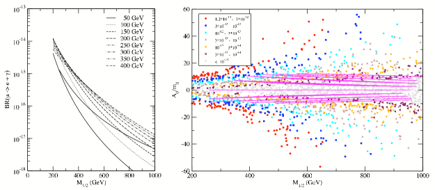
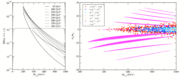
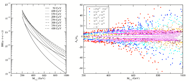
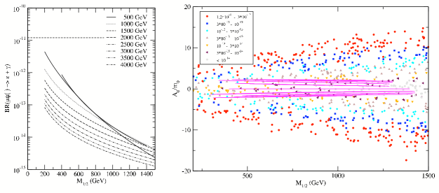
For each model in Figs. 3(a), 4(a), 5(a), 6(a), and 7(a), we plot curves with constant values of indicated for the BR21 branching ratios as functions of with the trilinear coupling at the GUT scale. The curve which cuts across the curves in each left-hand plot represents the WMAP dark matter constraint for this value of . The horizontal broken line indicates the present experimental upper limit for this branching ratio MEGA .
In Figs. 3(b), 4(b), 5(b), 6(b), and 7(b), we allow to depart from zero and show scatterplots of vs. . The points are color-coded as indicated according to the branching ratio intervals in which they fall, with all points below the present upper limit on the branching ratio. The soft parameter constraints in Eq. (33) have been imposed for the Monte Carlo selection of points. The continuous curves represent the WMAP dark matter constraints and are drawn in steps of 500 GeV from TeV to TeV.
(a) (b)
(a) (b)
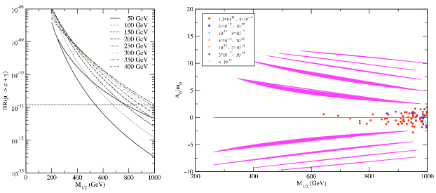
It is clear that the predicted branching ratio decreases as the universal soft gaugino mass at the GUT scale increases along the constant scalar mass curve. The Grimus-Kuhbock (GK) and Albright-Barr (AB) models will be probed first and then the Dermisek-Raby (DR) model by the MEG experiment, while the other two models are essentially beyond reach, if as depicted. One sees that higher values of BR21 are predicted for a given value of as increases. For the AB and GK models the experimental branching ratio greatly limits the allowed ranges of , while for the Chen-Mahanthappa (CM), Cai-Yu (CY), and DR models the dark matter constraints limit the allowed ranges of . In any case, the minimum predicted BR21 branching ratio occurs for .
One can also present similar scatter plots for the and decay modes. Since all three decay modes are intimately related in each model through the corresponding logarithmic terms such as that in Eq. (32), the same scatter points will appear with only the color-coding changed (assuming one imposes the BR21 experimental limit for each plot).
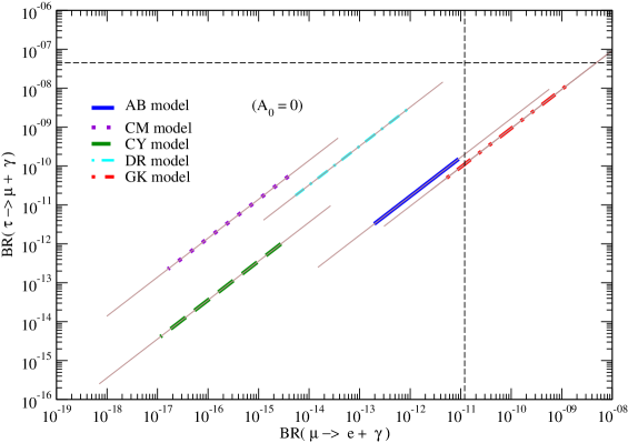
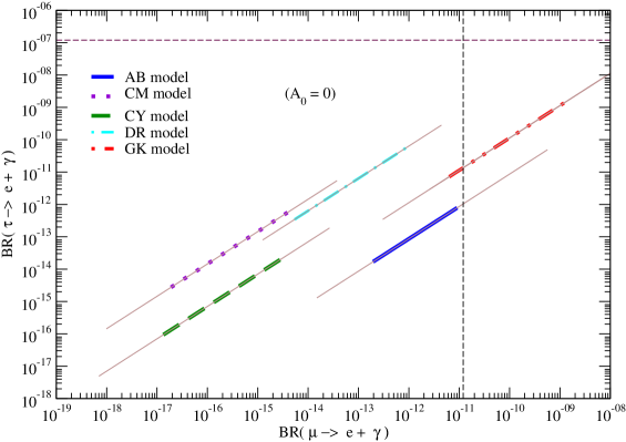
Instead, we present two log-log plots for the BR32 and BR31 branching ratios against that for BR21 in Figs. 8 and 9, where has again been imposed. The thin line segments for each model observe the soft parameters constraints imposed, while the heavier line segments observe the more restrictive WMAP dark matter constraints. The vertical dashed line reflects the present BR21 bound, while the horizontal dashed line refers to the present BR32 or BR31 experimental limit, respectively BRlimits . It is clear from these two plots that the ongoing MEG experiment stands the best chance of confirming the predictions for or eliminating the GK and AB models. Even with a super-B factory superB , the present experimental bounds on the BR32 and BR31 branching ratios can only be lowered by one or two orders of magnitude at most.
| Models | BR()/BR() | BR()/BR() | BR()/BR() |
|---|---|---|---|
| AB | 16.7 | 0.09 | 0.33 |
| CM | 171 | 0.11 | |
| CY | 400 | 6.5 | 0.11 |
| DR | 61.0 | 0.026 | |
| GK | 10.0 | 1.0 | 0.12 |
But recall that the line segments apply for the special case of . If one allows to depart from zero, the line segments will slide diagonally upward and toward the right along their presently depicted positions by amounts that can be estimated from Figs. 3 - 7. Hence only the lower limits on the branching ratios are robust in Figs. 8, 9 and 11. However, it is clear that ratios of the branching ratios remain fixed for each model for any allowed . We present these ratios for the and conversion branching ratios relative to the branching ratio in Table II. The spread in numbers for the ratios in different models appears to be greater than that anticipated by the authors of Ref. vogel for the class of models considered here.
| Models | ’s | BR21 | BR32 | BR() | |||
| Expt. | (GeV) | ||||||
| Limits | |||||||
| AB | 0.0020 | 5 | 5 | ||||
| () | |||||||
| CM | 0.013 | 10 | 12 | ||||
| () | |||||||
| CY | 0.0029 | 10 | 12 | ||||
| () | |||||||
| DR | 0.0024 | 50 | 2.5 | ||||
| () | |||||||
| GK | 0.00059 | 10 | 2 | ||||
| () | |||||||
In Table III we summarize the relevant findings from our study of the five models. The branching ratio ranges apply for the case and with the stricter WMAP dark matter constraints imposed. It is clear that the five predictive SUSY GUT models considered have very representative right-handed neutrino mass spectra and predictions for . The CM, DR, and GK models have massive hierarchical spectra with ranging from to GeV. The CY model, on the other hand, has a degenerate spectrum with GeV, while the AB model has degenerate and which can lead to resonant leptogenesis. The CM model has a relatively large prediction which should be observable at the upcoming reactor neutrino experiments, Double CHOOZ and Daya Bay. The AB, CY and DR models have similar predictions for which will make observation of oscillation somewhat marginal at those reactors and in the proposed NOA and T2K long-baseline experiments novat2k without a SuperBeam source. For the GK model, the observation of such a low prediction would only take place with a Neutrino Factory. But it is clear from Table III and the previous figures that the GK and AB models will be tested first with the MEG experiment. From our discussion it is then clear that the LFV branching ratios are more sensitive to large than to large in the models considered. In previous generic studies of SUSY GUT models, the rare branching ratios were nearly equally sensitive to each of the two parameters genericresults .
IV LEPTON FLAVOR VIOLATION IN CONVERSION
It is also of interest to consider lepton flavor violation in the to conversion process in Titanium, . While there is no such ongoing experiment, preliminary discussion is underway to propose one which will lower the present limit. We shall see that the conversion rate predictions relative to the muon capture process, , are such that all five models considered in this paper can potentially be eliminated, if no signal is observed.
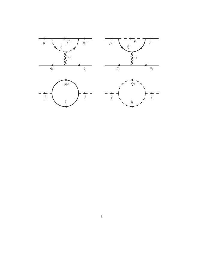
While predictions for the conversion process in the SM are infinitesimally small, large enhancements in the CMSSM framework again occur by virtue of massive super partners appearing in loop diagrams involving and Higgs penguins and boxes. Of these, Arganda, Herrero and Teixeira have shown that the penguin contributions dominate the others by at least two orders of magnitude AHT . The slepton-neutralino and sneutrino-chargino loop contributions to the penguins are shown in Fig. 10. The virtual massive and with their Yukawa couplings again appear in the slepton loops along with a higgsino or Higgs particle, respectively.
The complex formulas for lepton flavor violation in this process were first derived by Hisano, Moroi, Tobe, and Yamaguchi HMTY . If we restrict our attention to the penguin contribution as suggested by Arganda et al. AHT , one finds the conversion rate is given by
| (35) |
where here are form factors for the vertices connecting leptons of equal chirality, while are combinations of the electric dipole and magnetic dipole transition form factors previously denoted by . For a target, and the nuclear form factor is HMTY . In the case of the conversion process, we have explicitly carried out the full evolution running from the GUT scale to the scale. The conversion branching ratio is then obtained from the conversion rate above by scaling it with the capture rate on , which is quoted in mueconv as with the present experimental limit on the conversion branching ratio found to be .
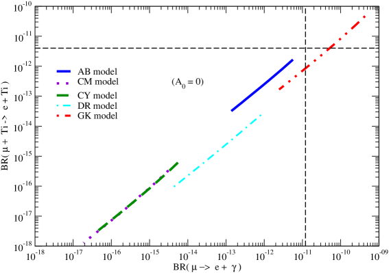
In Fig. 11. we show a plot of the conversion branching ratio vs. the branching ratio for each of the five models considered. We have limited the line segments by applying the WMAP dark matter constraints of Sec. III. It is clear that the GK and AB models would be tested first, followed by the DR, CY and CM models. In fact, a first generation conversion experiment may be able to reach a branching ratio of , while a second generation experiment may lower the limit from the present value down to mueprojection . If such proves to be the case and no signal is seen, all five models will be eliminated. Hence the conversion experiment is inherently more powerful than the MEG experiment looking for which is designed to reach a level of , sufficient only to eliminate the GK and AB models. The caveat, of course, is that MEG is now starting to take data, while no new conversion experiment has been approved to date.
V Conclusions
There have been many theoretical models constructed which aim to explain the neutrino masses and mixing patterns. While the predictions for the value of in these models may provide a way to distinguish some of these models, as shown in the survey over 63 models we have carried out in Ref. Albright:2006cw , the rare LFV processes, such as and conversion can provide an even more sensitive way to disentangle these models. We have investigated these rare processes in five SUSY SO(10) models that are currently still viable and highly predictive, making use of the allowed parameter space for the soft SUSY breaking parameters in the CMSSM framework. Utilizing the WMAP dark matter constraints, lower bounds on the branching ratios of these rare processes can be placed, and we find that at least three of the five models considered give rise to prediction for that will be tested at MEG. More interestingly, the next generation conversion experiment should be sensitive to the predictions of all five models, making it an even more robust way to test these models. While generic studies have emphasized the important dependence of the branching ratios on the reactor neutrino angle, , and the mass of the heaviest right-handed neutrino, we find the latter to be by far the more significant in the models tested.
ACKNOWLEDGMENTS
We thank Stephen Martin for making available to us his evolution program for the Yukawa couplings and soft SUSY breaking parameters. The work of M.-C.C. is supported, in part, by the National Science Foundation under Grant No. PHY-0709742. One of us (C.H.A.) thanks the members of the Theory Group at Fermilab for their kind hospitality. Fermilab is operated by the Fermi Research Alliance under contract No. DE-AC02-07CH11359 with the U.S. Department of Energy.
Note added.–After completion of this work, the authors of Ref. muecorrection informed us that a suppression factor should be applied to the lepton flavor violating branching ratios calculated in our paper. This suppression arises from a QED radiative correction to the effective dipole operators responsible for the rare decays. The multiplicative factor in question is given by , where , GeV is the sparticle mass scale responsible for the LFV, and for the rare radiative muon or tau decays. For , the correction amouts to roughly 0.15, so the branching ratio is about 0.85 times the rate given in the paper. The authors thank Andrzej Czarnecki and Ernest Jankowski for pointing out their earlier work to them.
References
- (1) Y. Ashie et al. (Super-Kamiokande Collaboration), Phys. Rev. D 71, 112005 (2005); J. Hosaka et al. (Super-Kamiokande Collaboration), Phys. Rev. D 73, 112001 (2006); B. Aharmin et al. (SNO Collaboration), Phys.Rev. C 72, 055502 (2005);
- (2) M. Apollonio et al. (CHOOZ Collaboration), Phys. Lett.B 420, 397 (1998); ibid., Eur. Phys. J C 27, 331 (2003); F. Boehm et al. (Palo Verde Collaboration), Phys.Rev. D 64, 112001(2001); T. Araki et al. (KamLAND Collaboration), Phys.Rev.Lett.94, 081801 (2005); S. Abe et al. (KamLAND Collaboration), arXiv:0801.4589.
- (3) M. Ahn et al. (K2K Collaboration), Phys. Rev. D 74, 072003 (2006); D.G. Michael et al. (MINOS Collaboration), Phys. Rev. Lett. 97, 191801 (2006); (MINOS Collaboration), arXiv:0708.1495.
- (4) M. Maltoni, T. Schwetz, M.A. Tortola and J.W.F. Valle, New J. Phys. 6, 122 (2004).
- (5) C.H. Albright and M.-C. Chen, Phys. Rev. D 74, 113006 (2006).
- (6) F. Borzumati and A. Masiero, Phys. Rev. Lett. 57, 961 (1986).
- (7) For recent reviews, see, e.g. M.-C. Chen and K. T. Mahanthappa, Int. J. Mod. Phys. A 18, 5819 (2003); AIP Conf. Proc. 721, 269 (2004); G. Altarelli and F. Feruglio, New J. Phys. 6, 106 (2004); S.F. King, Rept. Prog. Phys. 67, 107 (2004); Z.z. Xing, Int. J. Mod. Phys. A 19, 1 (2004); R.N.Mohapatra, New J. Phys. 6, 82 (2004); A. Yu. Smirnov, Int. J. Mod. Phys. A 19 1180 (2004); R.N. Mohapatra and A.Y. Smirnov, Ann. Rev. of Nucl. and Part. Sci., 56, 569 (2006); R.N. Mohapatra et al., Rep. Prog. Phys. 70, 1757 (2007); A. Strumia and F. Vissani, arXiv:hep-ph/0606054.
- (8) A. Masiero, S.K. Vempati, and O. Vives, Nucl. Phys. B649, 189 (2003); New J. Phys. 6, 202 (2004); F. Deppisch, H. Päs, A. Redelbach, R. Rückl, and Y. Shimizu, Eur. Phys. J. C 28, 365 (2003); F. Deppisch, H. Päs, R. Rückl, and A. Redelbach, Phys. Rev.D 73, 033004 (2006); E. Arganda and M.J. Herrero, Phys. Rev. D 73, 055003 (2006); L. Calibbi, A. Faccia, A. Masiero, and S.K. Vempati, J. High Energy Phys. 7, 012 (2007).
- (9) J.A. Casas and A. Ibarra, Nucl. Phys. B618, 171 (2001).
- (10) A. Kageyama, S. Kaneko, N. Shimoyama, and M. Tanimoto, Phys. Lett. B 527, 206 (2002); Q. Shafi and Z. Tavartkiladze, Nucl. Phys. B772, 133 (2007); B778, 216(E) (2007); S. Antusch and S.F. King, Phys. Lett. B 659, 640 (2008). An earlier test of one of the models considered in this work for the branching ratio was published in E. Jankowski and D.W. Maybury, Phys. Rev. D 70, 035004 (2004).
- (11) P. Minkowski, Phys. Lett. B 67, 421 (1977); T. Yanagida, in Proceedings of the Workshop on the Unified Theory and Baryon Number in the Universe, Tsukuba, Japan 1979, edited by O. Sawada and A. Sugamoto (KEK, Tsukuba, 1979), p. 95; M. Gell-Mann, P. Ramond, and R. Slansky, in Supergravity, edited by P. van Nieuwenhuizen and D. Z. Fredman (North-Holland, Amsterdam, 1979), p. 315; S.L. Glashow, in Proceedings of the 1979 Cargese Summer Institute on Quarks and Leptons, edited by M. Levy, J.-L. Basdevant, D. Speiser, J. Weyers, R. Gastmans, and M. Jacob (Plenum Press, New York, 1980), p. 687; R.N. Mohapatra and G. Senjanovic, Phys. Rev. Lett. 44, 912 (1980).
- (12) B. Pontecorvo, Zh. Eksp. Teor. Fiz. 33, 549 (1957) [Sov. Phys. JETP 6, 429 (1957)]; Z. Maki, M. Nakagawa and S. Sakata, Prog. Theor. Phys. 28, 870 (1962).
- (13) Review of Particle Physics, W.-M. Yao et al., J. Phys. G 33, 1 (2006).
- (14) K.S. Babu and R.N. Mohapatra, Phys. Rev. Lett. 70, 2845 (1993).
- (15) K.S. Babu and S.M. Barr, Phys. Lett. B 381, 202 (1996); C.H. Albright, K.S. Babu, and S.M. Barr, Phys. Rev. Lett. 81, 1167 (1998).
- (16) C.H. Albright, Phys. Lett. B 599, 285 (2004).
- (17) C.H. Albright and S.M. Barr, Phys.Rev. D 64, 073010 (2001).
- (18) C.H. Albright, Phys. Rev. D 72, 013001 (2005); 74, 039903(E) (2006).
- (19) A. Pilaftsis and T.E.J. Underwood, Nucl. Phys. B692, 303 (2004).
- (20) M.-C. Chen and K.T. Mahanthappa, Phys. Rev. D 70, 113013 (2004).
- (21) Y. Cai and H.-B. Yu, Phys. Rev. D 74, 115005 (2006).
- (22) R. Dermisek and S. Raby, Phys.Lett. B 622, 327 (2005).
- (23) W. Grimus and H. Kühbock, Phys. Lett. B 643, 182 (2006).
- (24) S.A. Dazley (Double CHOOZ Collaboration), in Proceedings of NuFACT05, Nucl. Phys. B, Proc. Suppl. 155, 231 (2006); J. Cao (Daya Bay Collaboration), ibid. 155, 229 (2006).
- (25) M. Apollonio et al. (CHOOZ Collaboration), Phys. Lett. B 420, 397 (1998); Eur. Phys. J. C 27, 331 (2003); cf. also F. Boehm et al. (Palo Verde Collaboration), Phys.Rev. D 64, 112001(2001).
- (26) B.W. Lee and R.E. Shrock, Phys. Rev. D 16, 1444 (1977).
- (27) A. Baldini, Nucl. Phys. B, Proc. Suppl. 168, 334 (2007).
- (28) M.L. Brooks et al. (MEGA Collaboration), Phys. Rev. Lett. 83, 1521 (1999).
- (29) For references to the CMSSM, cf. K.A. Olive, submitted to the SUSY07 proceedings arXiv:0709.3303.
- (30) J. Hisano, T. Moroi, K. Tobe, and M. Yamaguchi, Phys. Rev. 53, 2442 (1996).
- (31) S.T. Petcov, S. Profumo, Y. Takanishi, and C.E. Yaguna, Nucl. Phys. B676, 453 (2004).
- (32) D.N. Spergel et al. (WMAP Collaboration), Astrophys. J. Suppl. Ser. 170, 377 (2007).
- (33) P. Binetruy, G. Girardi, and P. Salati, Nucl. Phys. B237, 285 (1984); K. Griest and D. Seckel, Phys. Rev. D 43, 3191 (1991).
- (34) L.S. Stark, P. Häfliger, A. Biland, and F. Pauss, J. High Energy Phys. 0508, 059 (2005).
- (35) B. Aubert et al. (BABAR Collaboration), Phys. Rev. Lett. 96, 041801 (2006); 95, 041802 (2005); K. Abe et al. (Belle Collaboration), in Proceedings of the ICHEP06 Conference, Moscow, 2006.
- (36) A.G. Akeroyd et al. (SuperKEKB Physics Working Group), arXiv:hep-ex/0406071.
- (37) V. Cirigliano, A. Kurylov, M.J. Ramsey-Musolf, and P. Vogel, Phys. Rev. Lett. 93, 231802 (2004).
- (38) Y. Hayato et al. (T2K Collaboration), Nucl. Phys. B, Proc. Suppl. 143, 269 (2005); D.S. Ayres et al., Technical Design Report for the NOA Experiment E929 at Fermilab, 2007.
- (39) S. Antusch, E. Arganda, M.J. Herrero, and A.M. Teixeira, J. High Energy Phys. 11, 090 (2006), cf. Ref. generic .
- (40) E. Arganda, M.J. Herrero, and A.M. Teixeira, J. High Energy Phys. 10, 104 (2007).
- (41) C. Dohmen et al. (SINDRUM II Collaboration), Phys. Lett. B 317, 631 (1993).
- (42) W. Molzon, in Fermilab Program Planning Report Presented before the P5 Committee, January 2008.
- (43) A. Czarnecki and E. Jankowski, Phys. Rev. D 65, 113004 (2002).