Unbiased computation of transition times by pathway recombination
Abstract
In many systems, the time scales of the microscopic dynamics and macroscopic dynamics of interest are separated by many orders of magnitude. Examples abound, for instance nucleation, protein folding, and chemical reactions. For these systems, direct simulation of phase space trajectories does not efficiently determine most physical quantities of interest. The last decade has seen the advent of methods circumventing brute force simulation. For most dynamical quantities, these methods all share the drawback of systematical errors. We present a novel method for generating ensembles of phase space trajectories. By sampling small pieces of these trajectories in different phase space domains and piecing them together in a smart way using equilibrium properties, we obtain physical quantities such as transition times. This method does not have any systematic error and is very efficient; the computational effort to calculate the first passage time across a free energy barrier does not increase with the height of the barrier. The strength of the method is shown in the Ising model. Accurate measurements of nucleation times span almost ten orders of magnitude and reveal corrections to classical nucleation theory.
1 Introduction
The average time it takes a protein to fold, an undercooled liquid to crystallize, or a chemically active molecule to react, can in principle be obtained from brute force computer simulations, by simply starting several times in the unfolded, liquid or pre-reaction state and then integrating the dynamical equations in time until folding, crystallization or reaction takes place. However, the typical time scales of the microscopic dynamics and macroscopic dynamics of interest are often separated by many orders of magnitude; for such systems, direct simulation of relevant phase space trajectories is very inefficient, if at all possible. In the last decade, methods have been developed that sample transition pathways while circumventing brute force simulation, such as transition path sampling [1], transition interface sampling [2] and milestoning [3], but most dynamical quantities, e.g. the average transition time, are not provided by those methods or are provided with systematic errors. We present a method to determine such dynamical quantities, free from systematic errors and very efficient. Our method is generally applicable to systems with known equilibrium properties, consisting of two regions with locally stable states, separated from each other by a barrier, that may be very high.
2 Method
2.1 Problem
A typical question that can be addressed by our method is the following: if a system is in equilibrium in a region A of the phase space, what is the average time of first arrival in another region B? One should typically think of A and B as attracting basins in phase space, separated by a barrier. Examples of structures where such phenomena are found include nucleation, protein folding and chemical reactions. The simplest approach to answer such questions is by direct simulation: the system is started in A and evolved in time until B is reached, and this procedure is repeated many times to collect statistics. If, however, after leaving A returns to it are much more frequent than traversals to B, this direct simulation approach becomes very inefficient, since most of the computational effort is invested in dynamical trajectories from A back to A, rather than to B. Our method distributes the computational effort more efficiently, spending more time on actual traversals.
2.2 Sampling subtrajectories
The main idea behind our method is to sample different relatively small pieces of the phase space trajectories, which we call subtrajectories, and combine them with an appropriate weighting into complete trajectories. To classify the different subtrajectories, one should identify a slice M in phase space, such that every path connecting A and B has to pass through it. In the case of nucleation, for instance, the regions A, B and M could be the set of states in which the size of the largest nucleus is smaller than half, larger than twice, or equal to the critical nucleus size (or a good estimate of this). A long simulation trajectory can then be divided into subtrajectories, which are classified according to (1) their initial and final state (A or B) where the system resides at least the correlation time 111The correlation time can be different for the regions A and B, but for simplicity we take a single value for ., (2) whether M has been crossed (denoted by an ‘M’ between the initial and final state), and (3) whether the path crosses the other region without residing there longer than continuously or not (denoted by an ‘x’ or ‘o’ respectively). All these different types of subtrajectories are illustrated in figure 1. The figure also shows A- and B-subtrajectories that account for the time spent in A or B in excess of .
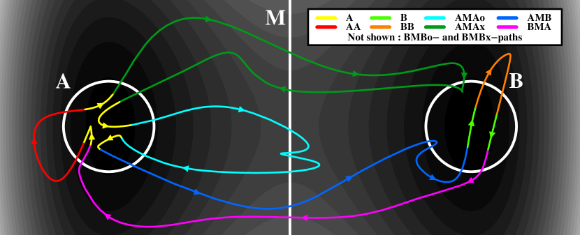
The different types of subtrajectories are generated by performing three different simulations. First, by starting in A, staying there for a time and evolving from then, ignoring the paths that go through M, the A- and AA-subtrajectories are sampled. Next, analogous simulations around B are performed to find the B- and BB-subtrajectories. Finally, simulations starting in M are performed to generate the subtrajectories through M. These subtrajectories through M are sampled by starting in M and evolving both forward and backward in time until a correlation time is spent in A or B continuously at both ends of the path. As shown in [4, 5], the starting points should be chosen from the set of points of first arrival in M from either A or B to sample the trajectories with the correct frequency. Because of time reversal symmetry, this can be achieved by sampling points on M from its equilibrium distribution, generating the trajectory by going forward and backward in time, and ignoring all paths that encounter M again on its backward part.
2.3 Recombination of subtrajectories
Now that the different types of subtrajectories are sampled, they should be recombined to generate complete phase space trajectories. These are concatinations of the subtrajectories, where the ones of the types AA, AMAo, AMAx, AMB, BB, BMBo, BMBx and BMA are intertwined with A- and B-subtrajectories. Recombination is based on the notion that in the stable regions in phase space A and B the system will mostly wander for a long time. If this time exceeds some value the system has lost memory of where it entered. Since after this time there is no correlation between the entrance and exit point of region A or B, any random recombination of these subtrajectories would constitute a valid trajectory. The subtrajectories of different simulations can be recombined if given the proper weights; that is why the method is efficient. In a straightforward simulation the subtrajectories crossing M typically are extremely rare, which strongly reduces statistical accuracy, but we generate additional subtrajectories through M by starting there and these subtrajectories can be combined with the AA- and BB-subtrajectories to sample long trajectories.
The weights for the different sets of subtrajectories can be determined from the condition that in the resulting long trajectories the system must be found in A, B or M with the correct equilibrium probabilities, , and . We assume these are known, either analytically or from other kinds of simulations, for instance parallel tempering [6], methods involving umbrella sampling [7, 8], cluster algorithms [9, 10] or the Wang-Landau method [11]. For each subtrajectory, we measure the time it spends in regions A, B and M. From these measurements we determine for each class of subtrajectories (where can be AA, AMAo, AMAx, AMB, BB, BMBo, BMBx and BMA) the average time spent in each region (where can be A, B or M) and these average times are also determined for the class M of all subtrajectories crossing M; these are the quantities . The notation without superscript will denote the average total time spent on one subtrajectory of class . Since these different subtrajectories are always preceded and succeeded by either an A- or B-subtrajectory, the time these latter subtrajectories take is also included in the times . The frequency with which a long trajectory enters subtrajectories of class is called . With these definitions, it follows immediately that the probabilities of being in the three regions satisfy the equalities
| (1a) | ||||
| (1b) | ||||
| (1c) | ||||
From these the subtrajectory frequencies may be expressed as:
| (2a) | ||||
| (2b) | ||||
| (2c) | ||||
During the simulations through M, the number of times that the specific classes of subtrajectories through M are encountered, are counted. These lead to the following relationships:
| (3) |
and these determine the remaining frequencies.
From the frequencies of the different subtrajectories we immediately obtain the probabilities for subtrajectories leaving A or B to be of specific type:
| (4a) | ||||
| (4b) | ||||
| (4c) | ||||
| (4d) | ||||
with and the analogous relations for the paths starting in B. Knowing these probabilities we can randomly recombine subtrajectories with the proper weights to generate complete trajectories.
2.4 Determining transition times
Depending on the exact quantity of interest, often the explicit recombination process can be skipped and replaced by a combination of appropriate averages over the subtrajectories. Here we specifically want to address the average transition time from A to B. Note that a traversal to B has to end with either an AMB- or AMAx-subtrajectory. To calculate the average transition time, we need to know the probabilities of finishing with an AMB- or AMAx-subtrajectory, the average numbers of times the AA- and AMAo-subtrajectories are traversed before this happens and the average times these subtrajectories take. This results in the following equation for the transition time:
| (5) |
The labels “first” are added to and , since the first time that region B is reached is relevant for the transition time, instead of the total time of the subtrajectory. These can also be measured during the simulations. We added an asterisk, to distinguish these times from the first arrival time of B for a system starting Boltzmann distributed in A; these times are the first arrival times of B for a system starting in A with another distribution, namely the distribution of points after being in A for a time . To obtain the real first arrival time , we must perform final simulations that start Boltzmann distributed in A until either time is spent in A, or arrival in B occurs. We call the average time until a time in A is spent , and the average time until arrival in B occurs ; these events happen with the probabilities and . The transition time from A to B, starting Boltzmann distributed in A, is then
| (6) |
2.5 Overview
Since the determination of the transition time from A to B involves multiple simulations in which a lot of quantities are measured, this section provides an overview of the different simulations including all measured quantities; these are presented in table 1. With these quantities measured, equations (2) - (6) yield the average time of first arrival in B for a system starting Boltmann distributed in A; other dynamical quantities can be obtained as well from different related equations.
| Simulations starting with a time in A | |
|---|---|
| The total time of an A-trajectory | |
| The total time of an AA-trajectory | |
| The time an AA-trajectory spends in A | |
| Simulations starting with a time in B | |
| The total time of a B-trajectory | |
| The total time of a BB-trajectory | |
| The time a BB-trajectory spends in B | |
| Simulations starting in M | |
| The total time of an M-trajectory | |
| , , | The time an M-trajectory spends in A, B or M, respectively |
| , | The first time that an AMAx- or AMB-trajectory arrives in B |
| The total number of M-trajectories | |
| , , | The number of AMAx-, AMAo- and AMB-trajectories, respectively |
| , , | The number of BMBx-, BMBo- and BMA-trajectories, respectively |
| Simulations starting Boltzmann distributed in A | |
| The time until a time is spent in A continuously | |
| The time to reach B without spending a time in A continuously | |
| , | The probabilities of starting with AA and AB |
3 Simple toy model
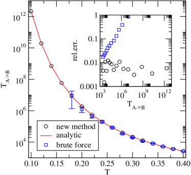
As a first test we applied this method to a system consisting of a 1010-lattice with a potential energy assigned to each site222The potential energy of the lattice sites is given by the function evaluated in the points with steps of . The sites and form potential minima, while the diagonal in between is around the potential maximum.. The dynamics consist of jumps of a single particle to neighboring sites with Metropolis [12] jump rates. “Regions” A and B are two opposing corners of the lattice, which are minima of the potential. M is the diagonal in between, which forms a ridge in the potential landscape. The simulations are performed for different values of the temperature. Their results are shown in figure 2, together with the results of brute force simulations. Both simulations lasted for one minute of CPU time. Also plotted is the exact transition time that is calculated by solving a set of linear equations.
The results are as expected: both our method and the brute force method sample the transition time without any systematic error. However, with our method the statistical error is constant as a function of the transition time, while the statistical errors of brute force simulation increase proportional to the inverse square root of the transition time, as the law of large numbers dictates (see the inset of figure 2).
4 Ising model
To show that the method does not only work efficiently in low-dimensional toy systems, we apply it to determine the nucleation time of a Ising model with spin-flip dynamics and Metropolis acceptance probabilities, for a large range of parameter values for and , i.e. the coupling constant and the external magnetization in units of .
Details of the simulations are as follows: we start in a metastable state consisting of spins antiparallel to the external magnetization. The coordinate used to characterize the regions A, B and M is the number of spins that are parallel to the external magnetization, and that have four neighbours which are also parallel to it. This turns out to be a much better reaction coordinate than for instance the size of the largest cluster of parallel spins. The convenient property of is that it can only change by a maximum of five; if the size of the largest cluster is taken as a reaction coordinate, it can undergo large changes due to the merging or splitting of clusters. To obtain the free energy as a function of we use successive umbrella sampling [13]: by restricting to either or , the free energy difference between and is determined; this process is repeated for increasing values of , until the free energy (as a function of ) returns to the value at . A typical result of this free energy sampling is shown in figure 3.
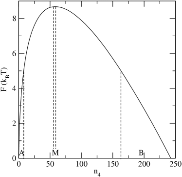
Next, the regions A, B and M are characterized in terms of . The region M is chosen at the top of the barrier and has width five, so that every nucleation trajectory intersects it. The regions A and B are such that the free energy barriers to its boundaries are . The motivation behind this is as follows: the barriers should be high enough that the system will linger in A and B long enough to lose correlation, but on the other hand low enough that it can be crossed by thermal activation to sample AA- and BB-trajectories; seems a reasonable choice for that. We will call region A the pre-nucleation state and B the nucleated state, since when the system arrives in B, it is extremely likely to continue to a stable state in which most spins are aligned with the external field. The regions A, B and M are also indicated in figure 3. With the regions A, B and M defined and the probabilities of being there known, the method can be applied to determine the nucleation times. In our simulations, we took a correlation time of 100 attemped spin flips per site. Equilibration inside region A and B is fast, and the system is certainly statistically uncorrelated within this time. We also verified this in simulations with and 500.
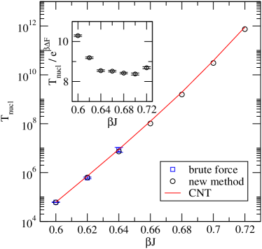
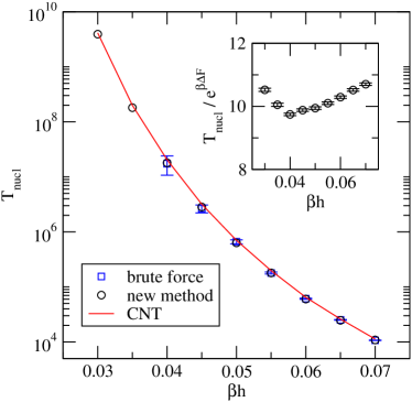
The resulting nucleation times are presented in figure 4. Note that the nucleation times span 10 orders of magnitude with constant relative statistical errors. For comparison, results of brute force simulations (if possible) and classical nucleation theory333Classical nucleation theory predicts that the nucleation time equals . The constant is fitted to the data. are also shown. The general trend is well captured by CNT. However, as shown in the insets, our method is accurate enough to reveal the shortcomings of CNT.
The computational effort in this calculation of the average nucleation time is approximately 13 hours of CPU time on an AMD-64 single-processor workstation for each set of temperature and field strength; one hour is spent for the determination of the free energy as a function of cluster size and 12 hours for the generation of the various subtrajectories and the nucleation time. An equal amount of computational effort was invested in the brute-force computations.
We would like to thank Henk van Beijeren for useful discussion.
 |
 |
References
- [1] C. Dellago, P.G. Bolhuis and P.L. Geissler, Adv. Chem. Phys. 123 (2002)
- [2] T.S. van Erp et al., J. Chem. Phys. 118, 7762 (2003)
- [3] A.K. Faradjian and Ron Elber, J. Chem. Phys. 120, 10880 (2004)
- [4] R.L. Jaffe, J.M. Henry and J.B. Anderson, J. Chem. Phys. 59, 1128 (1973)
- [5] J.B. Anderson, J. Chem. Phys. 60, 2566 (1974)
- [6] D.J. Earl and M.W. Deem, Phys. Chem. Chem. Phys. 7, 3910 (2005)
- [7] G. Torrie and J. Valleau, Chem. Phys. Lett. 28, 578 (1974)
- [8] G. Torrie and J. Valleau, J. Comp. Phys. 23, 187 (1977)
- [9] R.H. Swendsen and J.-S. Wang, Phys. Rev. Lett. 58, 86 (1987)
- [10] U. Wolff, Phys. Rev. Lett. 62, 361 (1989)
- [11] F. Wang and D.P. Landau, Phys. Rev. Lett. 86, 2050 (2001)
- [12] N. Metropolis et al., J. Chem. Phys. 21, 1087 (1953)
- [13] P. Virnau and M. Mueller, J. Chem. Phys. 120, 10925 (2004)