Chandra spectroscopy of the hot star $\beta$ Crucis and the discovery of a pre-main-sequence companion

Abstract

In order to test the O star wind-shock scenario for X-ray production in less luminous stars with weaker winds, we made a pointed 74 ks observation of the nearby early B giant, $\beta$ Cru (B0.5 III), with the Chandra High Energy Transmission Grating Spectrometer. We find that the X-ray spectrum is quite soft, with a dominant thermal component near 3 million K, and that the emission lines are resolved but quite narrow, with half-widths of 150 km s^-1. The forbidden-to-intercombination line ratios of Ne  ix and Mg  xi indicate that the hot plasma is distributed in the wind, rather than confined near the photosphere. It is difficult to understand the X-ray data in the context of the standard wind-shock paradigm for OB stars, primarily because of the narrow lines, but also because of the high X-ray production efficiency. A scenario in which the bulk of the outer wind is shock heated is broadly consistent with the data, but not very well motivated theoretically. It is possible that magnetic channeling could explain the X-ray properties, although no field has been detected on $\beta$ Cru. We detected periodic variability in the hard ($h\nu>1$ keV) X-rays, modulated on the known optical period of 4.58 hours, which is the period of the primary $\beta$ Cephei pulsation mode for this star. We also have detected, for the first time, an apparent companion to $\beta$ Cru at a projected separation of 4″. This companion was likely never seen in optical images because of the presumed very high contrast between it and $\beta$ Cru in the optical. However, the brightness contrast in the X-ray is only 3:1, which is consistent with the companion being an X-ray active low-mass pre-main-sequence star. The companion’s X-ray spectrum is relatively hard and variable, as would be expected from a post T Tauri star. The age of the $\beta$ Cru system (between 8 and 10 Myr) is consistent with this interpretation which, if correct, would add $\beta$ Cru to the roster of Lindroos binaries – B stars with low-mass pre-main-sequence companions.

1 Introduction

X-ray emission in normal O and early B stars is generally thought to arise in shocked regions of hot plasma embedded in the fast, radiation-driven stellar winds of these very luminous objects. High-resolution X-ray spectroscopy of a handful of bright O stars has basically confirmed this scenario (Kahn et al., 2001; Kramer et al., 2003; Cohen et al., 2006; Leutenegger et al., 2006). The key diagnostics are line profiles, which are Doppler broadened by the wind outflow, and the forbidden-to-intercombination ($\mathit{f}/i$) line ratios in helium-like ions of Mg, Si, and S, which are sensitive to the distance of the shocked wind plasma from the photosphere. Additionally, these O stars typically show rather soft spectra and little X-ray variability, both of which are consistent with the theoretical predictions of the line-driving instability (LDI) scenario (Owocki et al., 1988) and in contrast to observations of magnetically active coronal sources and magnetically channeled wind sources.

Table 1: Properties of $\beta$ Cru

MK Spectral Type	B0.5 III	Hiltner et al. (1969).
Distance (pc)	$108\pm 7$	Hipparcos (Perryman et al., 1997).
Age (Myr)	$8$ to $11$	Lindroos (1985); de Geus et al. (1989); Bertelli et al. (1994) and this work.
$\theta_{\rm LD}$ (mas)	$0.722\pm 0.023$	Hanbury Brown et al. (1974).
$M$ ($\mathrm{M_{\sun}}$)	$16$	Aerts et al. (1998).
$T_{\rm eff}$ (K)	$27,000\pm 1000$	Aerts et al. (1998).
log $g$ (cm s-2)	$3.6\pm 0.1$; $3.8\pm 0.1$	Aerts et al. (1998); Mass from Aerts et al. (1998) combined with radius.
$v\sin i$ (km s-1)	$35$	Uesugi & Fukuda (1982).
$L$ ($\mathrm{L_{\sun}}$)	$3.4\times 10^{4}$	Aerts et al. (1998).
$R$ ($\mathrm{R_{\sun}}$)	$8.4\pm 0.6$	From distance (Perryman et al., 1997) and $\theta_{\rm LD}$ (Hanbury Brown et al., 1974).
Pulsation periods (hr)	4.588, 4.028, 4.386, 6.805, 8.618	Aerts et al. (1998); Cuypers et al. (2002).
$\dot{M}$ ($\mathrm{M_{\sun}~{}{\mathrm{y}r^{-1}}}$)	$10^{-8}$	Theoretical calculation, using Abbott (1982).
${\dot{M}}q$ ($\mathrm{M_{\sun}~{}{\mathrm{y}r^{-1}}}$)	$10^{-11}$	Product of mass-loss rate and ionization fraction of C iv (Prinja, 1989).
$v_{\infty}$ (km s-1)	$2000$	Theoretical calculation, using Abbott (1982).
$v_{\infty}$ (km s-1)	$420$	Based on C iv absorption feature blue edge (Prinja, 1989).

In order to investigate the applicability of the LDI wind-shock scenario to early B stars, we have obtained a pointed Chandra grating observation of a normal early B star, $\beta$ Crucis (B0.5 III). The star has a radiation-driven wind but one that is much weaker than those of the O stars that have been observed with Chandra and XMM-Newton. Its mass-loss rate is at least two and more likely three orders of magnitude lower than that of the O supergiant $\zeta$ Pup, for example. Our goal is to explore how wind-shock X-ray emission changes as one looks to stars with weaker winds, in hopes of shedding more light on the wind-shock mechanism itself and also on the properties of early B star winds in general. We will apply the same diagnostics that have been used to analyze the X-ray spectra of O stars: line widths and profiles, $\mathit{f}/i$ ratios, temperature and abundance analysis from global spectral modeling, and time-variability analysis.

There are two other properties of this particular star that make this observation especially interesting: $\beta$ Cru is a $\beta$ Cephei variable, which will allow us to explore the potential connection among pulsation, winds, and X-ray emission; and the fact that there are several low-mass pre-main-sequence stars in the vicinity of $\beta$ Cru. This second fact became potentially quite relevant when we unexpectedly discovered a previously unknown X-ray source four arc seconds from $\beta$ Cru in the Chandra data.

In the next section, we discuss the properties and environment of $\beta$ Cru. In §3 we present the Chandra data. In §4 we analyze the spectral and time-variability properties of $\beta$ Cru. In §5 we perform similar analyses of the newly discovered companion. We discuss the implications of the analyses of both $\beta$ Cru and the companion as well as summarize our conclusions in §6.

2 The $\beta$ Cru system

One of the nearest early-type stars to Earth, $\beta$ Cru is located at a distance of only 108 pc (Perryman et al., 1997). With a spectral type of B0.5, this makes $\beta$ Cru – also known as Becrux, Mimosa, and HD 111123 – extremely bright. In fact, it is the 19th brightest star in the sky in the V band, and as a prominent member of the Southern Cross (Crux), it appears in the flags of at least five nations in the Southern Hemisphere, including Australia, New Zealand, and Brazil.

The fundamental properties of $\beta$ Cru have been extensively studied and, in our opinion, quite well determined now, although binarity and pulsation issues make some of this rather tricky. In addition to the Hipparcos distance, there is an optical interferometric measurement of the star’s angular diameter (Hanbury Brown et al., 1974), and thus a good determination of its radius. It is a spectroscopic binary (Heintz, 1957) with a period of 5 years (Aerts et al., 1998). Careful analysis of the spectroscopic orbit, in conjunction with the brightness contrast at 4430 Å from interferometric measurements (Popper, 1968) and comparison to model atmospheres, enable determinations of the mass, effective temperature, and luminosity of $\beta$ Cru (Aerts et al., 1998). The log $g$ value and mass imply a radius that is consistent with that derived from the angular diameter and parallax distance, giving us additional confidence that the basic stellar parameters are now quite well constrained. The projected rotational velocity is low ($v\sin i=35$ km s^-1), but the inclination is also likely to be low. Aerts et al. (1998) constrain the orbital inclination to be between 15° and 20°, and binary orbital and equatorial planes are well aligned for binaries with $a\la 10$ AU (Hale, 1994). This implies $v_{\mathrm{rot}}\approx 120$ km s^-1 and combined with $\rm R_{\ast}=8.4~{}\mathrm{R_{\sun}}$, the rotational period is $P_{\mathrm{rot}}\approx 3\aas@@fstack{d}6$. The star’s properties are summarized in Table 1.

With $T_{\rm eff}=27,000\pm 1000$ K, $\beta$ Cru lies near the hot edge of the $\beta$ Cephei pulsation strip in the HR diagram (Stankov & Handler, 2005). Three different non-radial pulsation modes with closely spaced periods between 4.03 and 4.59 hours have been identified spectroscopically (Aerts et al., 1998). Modest radial velocity variations are seen at the level of a few km s^-1 overall, with some individual pulsation components having somewhat larger amplitudes (Aerts et al., 1998). The three modes are identified with azimuthal wavenumbers $\ell=1$, 3, and 4, respectively (Aerts et al., 1998; Cuypers et al., 2002). The observed photometric variability is also modest, with amplitudes of a few hundredths of a magnitude seen only in the primary pulsation mode (Cuypers, 1983). More recent, intensive photometric monitoring with the star tracker aboard the WIRE satellite has identified the three spectroscopic periods and found two additional very low amplitude (less than a millimagnitude), somewhat lower frequency components (Cuypers et al., 2002).

The wind properties of $\beta$ Cru are not very well known, as is often the case for non-supergiant B stars. The standard theory of line-driven winds (Castor et al., 1975) (CAK) enables one to predict the mass-loss rate and terminal velocity of a wind given a line list and stellar properties. There has not been much recent work on applying CAK theory to B stars, as the problem is actually significantly harder than for O stars, because B star winds have many fewer constraints from data and the ionization/excitation conditions are more difficult to calculate accurately. With those caveats, however, we have used the CAK parameters from Abbott (1982) and calculated the mass-loss rate and terminal velocity using the stellar parameters in Table 1 and the formalism described by Kudritzki et al. (1989). The mass-loss rate is predicted to be about $10^{-8}$ $\mathrm{M_{\sun}~{}{\mathrm{y}r^{-1}}}$ and the terminal velocity, $v_{\infty}\approx 2000$ km s^-1. There is some uncertainty based on the assumed ionization balance of helium, as well as the uncertainty in the stellar properties (gravity, effective temperature, luminosity), and whatever systematic errors exist in the line list. The wind models of Vink et al. (2000) also predict a mass-loss rate close to $10^{-8}$ $\mathrm{M_{\sun}~{}{\mathrm{y}r^{-1}}}$ for $\beta$ Cru.

Interestingly, IUE observations show very weak wind signatures - in Si iv and C iv, with no wind signature at all seen in Si iii. The C iv doublet near 1550 Å has a blue edge velocity of only 420 km s^-1, while the blue edge velocity of the Si iv line is slightly smaller. The products of the mass-loss rate and the ionization fraction of the relevant ion are roughly $10^{-11}$ $\mathrm{M_{\sun}~{}{\mathrm{y}r^{-1}}}$ for both of these species (Prinja, 1989). Either the wind is much weaker than CAK theory (using Abbott’s parameters) predicts or the wind has a very unusual ionization structure. We will come back to this point in §6.

$\beta$ Cru is most likely a member of the Lower Centaurus Crux (LCC) subgroup of the Sco-Cen OB association. Although a classical member of LCC (e.g, Blaauw, 1946), $\beta$ Cru was not selected as an LCC member by de Zeeuw et al. (1999) in their analysis of Hipparcos data. However, the timespan of the Hipparcos proper motion measurement (4 years) is similar to the 5-yr orbital period of the spectroscopic binary companion. The rate of orbital angular displacement of $\beta$ Cru is similar to its proper motion, which likely influenced the Hipparcos proper-motion measurement. For this reason, de Zeeuw et al. (1999) suspect that $\beta$ Cru is an LCC member even though it is not formally selected as one by their criteria, and indeed Hoogerwerf (2000) find that $\beta$ Cru is an LCC member based on longer-time-baseline proper motion measurements.

The age of $\beta$ Cru is also roughly consistent with LCC membership, given the uncertainty about the age(s) of the LCC itself. The age of LCC has been variously found to be from 10–12 Myr (de Geus et al., 1989) to 17–23 Myr (Mamajek, Meyer, & Liebert, 2002), and more recent work has found evidence for an age spread and spatial substructure within the region (Preibisch & Mamajek, 2007). $\beta$ Cru has been claimed to have an evolutionary age of 8 Myr (Lindroos, 1985), though the distance was much more uncertain when this work was done. Using our adopted stellar parameters (Table 1), $\beta$ Cru has an age of 8–10 Myr when plotted on the evolutionary tracks of Bertelli et al. (1994). As such, $\beta$ Cru has evolved off the main sequence, but not very far. Its spectroscopic binary companion is a B2 star that is still on the main sequence (Aerts et al., 1998), and the projected X-ray companion discussed below, if it is a physical companion, is likely to be a pre–main-sequence (PMS) star. There are two other purported wide visual companions ($\beta$ Cru B and C) listed in the Washington Double Star catalog (Worley & Douglass, 1997), with separations of 44″ and 370″, although they are almost certainly not physical companions of $\beta$ Cru (Lindroos, 1985).

A small group of X-ray bright pre–main-sequence stars within about a degree of $\beta$ Cru was discovered by ROSAT (Park & Finley, 1996). These stars are likely part of the huge low-mass PMS population of the LCC (Feigelson & Lawson, 1997). They have recently been studied in depth (Alcalá et al., 2002), and four of the six have been shown to be likely post-T-Tauri stars (and one of those is a triple system). They have ${\mathrm{H}{\alpha}}$ in emission, strong Li 6708 Å absorption, and radial velocities consistent with LCC membership. Assuming that they are at the same distance as $\beta$ Cru, their ages from PMS evolutionary tracks are 4–10 Myr. This is somewhat younger than LCC ages derived from the more massive members, but this is consistent with a larger pattern of systematic age differences for LCC members of different masses and may indicate systematic errors in the evolutionary tracks (Preibisch & Mamajek, 2007).

3 The Chandra data

We obtained the data we report on in this paper in a single long pointing on 28 May 2002, using the Chandra Advanced CCD Imaging Spectrometer in spectroscopy mode with the High Energy Transmission Grating Spectrometer (ACIS-S/HETGS configuration) (Canizares et al., 2005). The ACIS detector images the dispersed spectra from two grating components of the HETGS, the medium energy grating (MEG) and the high energy grating (HEG). The mirror, grating, and detector combination has significant response on a wavelength range extending roughly from 2 Å to 40 Å, though with a total (including both negative and positive orders) effective area of only about 10 cm². The spectral resolution exceeds $\lambda/\Delta{\lambda}=1000$ at the long-wavelength end of each grating’s spectral range, and decreases toward shorter wavelengths. The spatial resolution of Chandra is excellent, with the core of the point spread function having a full width of less than half an arcsecond. Properties and characteristics of the telescope and detector are available via the Proposers’ Observatory Guide (CXC, 2007).

We reran the pipeline reduction tasks in the the standard Chandra Interactive Analysis of Observations (CIAO) software, version 3.3, using the calibration database, CALDB 3.2, and extracted the zeroth order spectrum and the dispersed first order MEG and HEG spectra of both $\beta$ Cru and the newly discovered companion. The zeroth order spectrum of a source in the Chandra ACIS-S/HETGS is an image created by source photons that pass directly through the transmission gratings without being diffracted. The ACIS CCD detectors themselves have some inherent energy discrimination so a low-resolution spectrum can be produced from these zeroth-order counts.

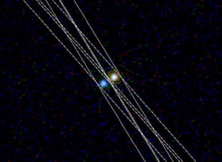
Figure 1: Image of the center of the ACIS detector, showing the zeroth order spectra of $\beta$ Cru and its newly discovered companion. North is up and east is left. $\beta$ Cru is the source to the northwest. Its position in the ACIS detector is coincident with the optical position of $\beta$ Cru to within the positional accuracy of Chandra. The companion is to the southeast, at a separation of 4.0″ and with a position angle relative to $\beta$ Cru of $120^{\circ}$. The extraction regions for the MEG and HEG (both positive and negative orders) are indicated for both sources. It can be seen in this image that the position angle is nearly perpendicular to the dispersion directions (for both the MEG and HEG) and thus that the dispersed spectra of the two sources can be separated. In the on-line color version of this figure, hard counts (h$\nu>1$ keV) are blue, soft counts (h$\nu<0.5$ keV) are red, and counts with intermediate energies are green. It can easily be seen in the color image that the X-ray emission of the companion is dramatically harder than that of $\beta$ Cru.

The zeroth order spectrum of each source has very little pileup ($\sim 7$% for $\beta$ Cru), and the grating spectra have none. The HEG spectra and the higher order MEG spectra have almost no source counts, so all of the analysis of dispersed spectra we report on here involves just the MEG $\pm$1 orders. There were typically five to ten pixels across each emission line, and few lines have even 100 counts per line. The random errors on the source count rates are dominated by Poisson photon-counting noise. Thus even the strongest lines have signal-to-noise ratios per pixel of only several. The background (instrumental and astrophysical) is negligible. We made observation-specific response matrix files (rmfs; encoding the energy-dependent spectral response) and grating ancillary response files (garfs; containing information about the wavelength-dependent effective area) and performed our spectral analysis in both XSPEC 11.3.1 and ISIS 1.4.8. We performed time-variability analysis on both binned light curves and unbinned photon event tables using custom-written codes.

The observation revealed only a small handful of other possible sources in the field, which we identified using the CIAO task celldetect with the threshold parameter set to a value of 3. We extracted background-subtracted source counts from three weak sources identified with this procedure. Their signal-to-noise ratios are each only slightly above 3. The only other bright source in the field of view is one just 4$\aas@@fstack{\prime\prime}$0 to the southeast of $\beta$ Cru at a position angle of 120 degrees, which is clearly separated from $\beta$ Cru, as can be seen in Fig. 1. The position angle uncertainty is less than a degree based on the formal errors in the centroids of the two sources, and the uncertainty in the separation is less than 0$\aas@@fstack{\prime\prime}$1. We present the X-ray properties of this source in §5 and argue in §6 that it is most likely a low-mass PMS star in orbit around $\beta$ Cru. The B star that dominates the optical light of the $\beta$ Cru system and which is the main subject of this paper should formally be referred to as $\beta$ Cru A (with spectroscopic binary components 1 and 2). The companion at a projected separation of 4″ will formally be known as $\beta$ Cru D, since designations B and C have already been used for the purported companions listed in the Washington Double Star Catalog, mentioned in the previous section. Throughout this paper, we will refer to $\beta$ Cru A and D simply as “$\beta$ Cru” and “the companion.”

Table 2: Point sources in the field

Name(s)	RA	Dec.	total counts	X-ray flux
	(J2000)	(J2000)		($10^{-14}$ ergs s-1 cm-2)
$\beta$ Cru A; Mimosa; Becrux; HD 111123	$12~{}47~{}43.35$	$-59~{}41~{}19.2$	$3803\pm 12$	$186\pm 1$
$\beta$ Cru D; CXOU J124743.8-594121	$12~{}47~{}43.80$	$-59~{}41~{}21.3$	$1228\pm 12$	$57.3\pm.6$
CXOU J124752.5-594345	$12~{}47~{}52.53$	$-59~{}43~{}45.8$	$25.9\pm 8.6$	$1.58\pm.52$
CXOU J124823.9-593611	$12~{}48~{}23.91$	$-59~{}36~{}11.8$	$47.4\pm 10.4$	$3.32\pm.73$
CXOU J124833.2-593736	$12~{}48~{}33.22$	$-59~{}37~{}36.8$	$29.6\pm 9.8$	$2.23\pm.74$

We summarize the properties of all the point sources on the ACIS chips in Tab. 2. We note that the other three sources have X-ray fluxes about two orders of magnitude below those of $\beta$ Cru and the newly discovered companion. They show no X-ray time variability, and their spectra have mean energies of roughly 2 keV and are fit by absorbed power laws. These properties, along with the fact that they have no counterparts in the 2MASS point source catalog, indicate that they are likely AGN. We did not detect any of the pre-main-sequence stars seen in the ROSAT observation because none of them fell on the ACIS CCDs. We also note that there is no X-ray source detected at the location of the wide visual companion located 44″ from $\beta$ Cru, $\beta$ Cru C, which is no longer thought to be physically associated with $\beta$ Cru (Lindroos, 1985). We place a $1\sigma$ upper limit of 7 source counts in an extraction region at the position of this companion. This limit corresponds to an X-ray flux more than two orders of magnitude below that of $\beta$ Cru or its X-ray bright companion.

The position angle of the newly discovered companion is oriented almost exactly perpendicular to the dispersion direction of the MEG for this particular observation. This can be seen in Fig. 1, where parts of the rectangular extraction regions for the dispersed spectra are indicated. We were thus able to cleanly extract not just the zeroth order counts for both sources but also the MEG and HEG spectra for both sources. We visually inspected histograms of count rates versus pixel in the cross-dispersion direction at the locations of several lines and verified that there was no contamination of one source’s spectrum by the other’s. We analyze these first-order spectra as well as the zeroth-order spectra and the timing information for both sources in §4 and §5.

4 Analysis of $\beta$ Cru

4.1 Spectral Analysis

The dispersed spectrum of $\beta$ Cru is very soft and relatively weak. We show the co-added negative and positive first-order MEG spectra in Fig. 2, with the strong lines labeled. The softness is apparent, for example, in the relative weakness of the Ne x Lyman-$\alpha$ line at 12.13 Å compared to the Ne ix He_α complex near 13.5 Å, and indeed the lack of any strong lines at wavelengths shorter than 12 Å.

Figure 2: The MEG spectrum of $\beta$ Cru, with negative and positive first orders coadded and emission lines identified by ion. Bins are 5 mÅ wide, and each emission line spans several bins. We show a smoothed version of these same data in Fig. 4.

4.1.1 Global thermal spectral modeling

We characterized the temperature and abundance distributions in the hot plasma on $\beta$ Cru by fitting Astrophysical Plasma Emission Code (APEC) thermal, optically thin, equilibrium plasma spectral emission models (Smith et al., 2001) to both the zeroth and first order spectra. We included a model for pileup in the fit to the zeroth order spectrum (Davis, 2001). For the dispersed MEG spectrum, we adaptively smoothed the data for the fitting in ISIS. This effectively combines bins with very few counts to improve the statistics in the continuum. We also modified the vAPEC (“v” for variable abundances) implementation in ISIS to allow the helium-like forbidden-to-intercombination line ratios to be free parameters (the so-called ${\mathcal{G}}$ parameter, which is the ratio of the forbidden plus intercombination line fluxes to the flux in the resonance line, ${\mathcal{G}}\equiv\frac{f+i}{r}$, was also allowed to be a free parameter). We discuss these line complexes and their diagnostic power later in this subsection. The inclusion of these altered line ratios in the global modeling was intended at this stage simply to prevent these particular lines from influencing the fits in ways that are not physically meaningful.

The number of free parameters in a global thermal model like APEC can quickly proliferate. We wanted to allow for a non-isothermal plasma, non-solar abundances, and thermal and turbulent line broadening (in addition to the non-standard forbidden-to-intercombination line ratios). However, we were careful to introduce new model parameters only when they were justified. So, for example, we only allowed non-solar abundances for species that have several emission lines in the MEG spectrum. And we found we could not rely solely on the automated fitting procedures in XSPEC and ISIS because information about specific physical parameters is sometimes contained in only a small portion of the spectrum, so that it has negligible effect on the global fit statistic.

We thus followed an iterative procedure in which we first fit the zeroth-order spectrum with a solar-abundance, two-temperature APEC model. We were able to achieve a good fit with this simple type of model, but when we compared the best fit model to the dispersed spectrum, systematic deviations between the model and data were apparent. Simply varying all the free model parameters to minimize the fit statistic (we used both the Cash C statistic (Cash, 1979) and $\chi^{2}$, periodically comparing the results for the two statistics) was not productive because, for example, the continuum in the MEG spectrum contains many more bins than do the lines, but the lines generally contain more independent information. And for some quantities, like individual abundances, only a small portion of the spectrum shows any dependence on that parameter, so we would hold other model parameters fixed and fit specific parameters on a restricted subset of the data. Once a fit was achieved, we would hold that parameter fixed and free others and refit the data as a whole.

Ultimately, we were able to find a model that provided a good fit to the combined data, both zeroth-order and dispersed spectra. The model parameters are listed in Tab. 3, and the model is plotted along with the zeroth order spectrum in Fig. 3 and the adaptively smoothed first order MEG spectrum in Fig. 4. There are some systematic deviations between the model and the data, but overall the fit quality is good, with $\chi^{2}_{\nu}=1.09$ for the combined data. The formal confidence limits on the fit parameters are unrealistically narrow, at least partly because the statistical error cannot be fully accounted for. For example, the abundance determinations are each made on narrow wavelength intervals and thus the temperature cannot reliably be allowed to vary along with the abundances in the confidence limit testing procedure. We return to this point below when we discuss the abundance determinations. The overall result, that a thermal model with a dominant temperature near 3 million K and an emission measure of $\sim 3.5\times 10^{53}$ cm^-3 and abundances that overall are slightly sub-solar is required to fit the data, is quite robust.

The model we present provides a better fit for the first-order MEG spectrum, which has 443 bins when we adaptively smooth it. The model gives $\chi_{\nu}^{2}=1.00$ for the first order MEG spectrum alone, while it gives $\chi_{\nu}^{2}=1.42$ for the zeroth order spectrum alone, which has 90 bins. We suspect the relatively poor agreement between the CCD spectrum and the MEG spectrum stems from the small, but non-zero, transmission of red optical light through the MEG and HEG gratings and through the ACIS optical blocking filter (Wolk, 2002). Being so bright, $\beta$ Cru is more susceptible to this effect than nearly any other object. We examined the Chandra ACIS spectrum of Vega, which is very bright in the optical and X-ray dark. Its CCD spectrum, which is presumably due entirely to the optical contamination, looks very similar to the excess above the model seen in the $\beta$ Cru spectrum. The optical contamination is particularly noticeable in the $0.22-0.5$ keV ACIS-S band, which we have chosen not to model. There appears to be some contamination up to $\sim 0.7$ keV, however.

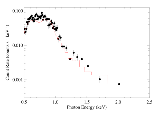
Figure 3: The best-fit two-temperature, variable abundance thermal spectral (APEC) model (dotted line), corrected for pileup, superimposed on the zeroth-order spectrum of $\beta$ Cru. The model shown is the best-fit model fit to both the zeroth and first order spectra, with parameters listed in Tab. 3. It seems likely that some of the systematic deviations in the softer channels are due to optical contamination, as discussed in §4.1.1.

In Fig. 4, where we show our global best-fit model superimposed on the adaptively smoothed MEG spectrum, the continuum is seen to be well reproduced and the strengths of all but the very weakest lines are reproduced to well within a factor of two. It is interesting that no more than two temperature components are needed to fit the data; the continuum shape and line strengths are simultaneously explained by a strong 2.5 million K component and a much weaker 6.5 million K component.

The constraints on abundances from X-ray emission line spectra are entangled with temperature effects. So, it is important to have line strength measurements from multiple ionization stages. This is strictly only true in the MEG spectrum for O and Ne, but important lines of Mg, Si, and Fe from non-dominant ionization stages would appear in the spectrum if they were strong, so the non-detections of lines of Mg  xii, Si  xiv, and Fe  xviii provide information about the abundances of these elements. These five elements are the only ones for which we report abundances derived from the model fitting (see Tab. 3). We allowed the nitrogen abundance to be a free parameter of the fit as well, but do not report its value, as it is constrained by only one detected line in the data. The uncertainties on these abundances are difficult to reliably quantify (because of the interplay with the temperature distribution) but they are probably less than a factor of two, based on our experience varying these parameter values by hand. They are certainly somewhat larger than the formal confidence limits listed in Tab. 3, but even given that, there is an overall trend of slightly subsolar abundances, consistent with a value perhaps somewhat above half solar. Only the oxygen abundance seems to be robustly and significantly sub-solar. We note, however, that in general, the abundances we find are significantly closer to solar than those reported by Zhekov & Palla (2007).

Table 3: Best-fit parameters for the two-temperature APEC thermal equilibrium spectral model

parameter	value	90% confidence limits
$T_{\mathrm{1}}$ (K)	$2.5\times 10^{6}$	$2.4:2.6\times 10^{6}$
${\mathcal{E}M}_{\mathrm{1}}$ (cm-3)	$3.3\times 10^{53}$	$3.1:3.5\times 10^{53}$
$T_{\mathrm{2}}$ (K)	$6.5\times 10^{6}$	$6.2:6.8\times 10^{6}$
${\mathcal{E}M}_{\mathrm{2}}$ (cm-3)	$2.8\times 10^{52}$	$2.3:3.3\times 10^{52}$
$v_{\mathrm{turb}}$ (km s-1)	180	90:191
O	0.35	0.30:0.40
Ne	0.78	0.70:0.99
Mg	0.52	0.29:0.62
Si	1.05	0.68:1.56
Fe	0.80	0.70:0.90

The abundances are the (linear) fraction of the solar abundance, according to Anders & Grevesse (1989).

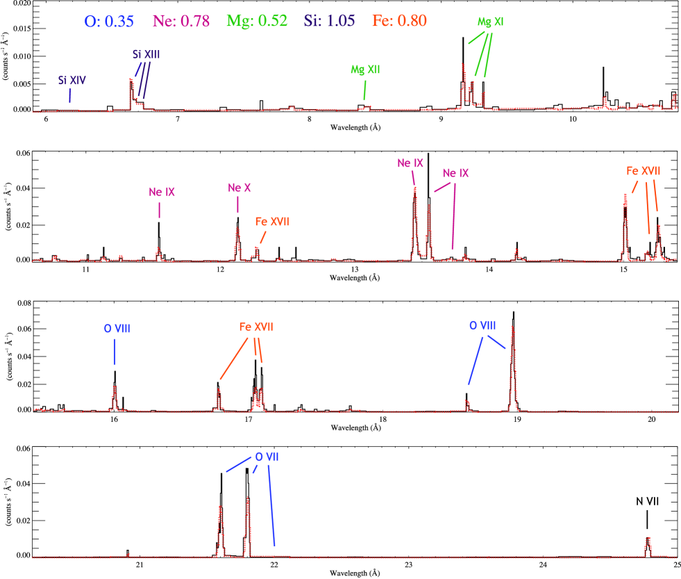
Figure 4: The best-fit two-temperature, variable abundance thermal spectral (vAPEC) model (red, dotted line; parameters listed in Tab. 3; same model as shown in Fig. 3), superimposed on the adaptively smoothed co-added MEG first-order spectrum of $\beta$ Cru. Emission lines are labeled and color coded according to element, with the abundances of each element listed at the top of the figure. Some non-detected lines are labeled, including the forbidden line of O  vii near 22.1 Å and the Lyman-alpha line of Si  xiv near 6.2 Å.

In all fits we included ISM absorption assuming a hydrogen column density of $3.5\times 10^{19}$ cm^-2. This value is consistent with the very low $E(B-V)=0.002\pm.011$ (Niemczura & Daszynska-Daszkiewicz, 2005) and is the value determined for the nearby star HD 110956 (Fruscione et al., 1994). This low ISM column produces very little attenuation, with only a few percent of the flux absorbed even at the longest Chandra wavelengths. The overall X-ray flux of $\beta$ Cru between $0.5$ keV and 8 keV is $1.86\pm.01\times 10^{-12}$ ergs s^-1 cm^-2, implying $L_{\rm x}=2.6\times 10^{30}$ ergs s^-1, which corresponds to $\log L_{\rm x}/L_{\rm Bol}=-7.72$.

4.1.2 Individual emission lines: strengths and widths

Even given the extreme softness of the dispersed spectrum shown in Figs. 2, 3, and 4, the most striking thing about these data is the narrowness of the X-ray emission lines. Broad emission lines in grating spectra of hot stars are the hallmark of wind-shock X-ray emission (Kahn et al., 2001; Cassinelli et al., 2001; Kramer et al., 2003; Cohen et al., 2006). While the stellar wind of $\beta$ Cru is weaker than that of O stars, it is expected that the same wind-shock mechanism that operates in O stars is also responsible for the X-ray emission in these slightly later-type early B stars (Cohen et al., 1997). The rather narrow X-ray emission lines we see in the MEG spectrum of $\beta$ Cru would thus seem to pose a severe challenge to the application of the wind-shock scenario to this early B star. We will quantify these line widths here, and discuss their implications in §6.

Table 4: Emission Lines in the HETGS/MEG Spectrum

ion	$\lambda_{{\rm lab}}$	$\lambda_{{\rm obs}}$	shift	half-width	normalization	corrected flux
	(Å)	(Å)	(mÅ)	(mÅ)	(10-6 ph s-1 cm-2)	(10-15 erg s-1 cm-2)
Si  xiii	6.6479 (r)	$-$	$-$	$1.7^{+3.5}_{-1.7}$	$1.06^{+0.41}_{-0.34}$	$3.15^{+1.22}_{-1.01}$
Si  xiii	6.6882 (i)	$-$	$-$	$1.7$	$0.31^{+0.26}_{-0.17}$	$0.93^{+0.78}_{-0.51}$
Si  xiii	6.7403 (f)	$-$	$-$	$1.7$	$0.77^{+0.33}_{-0.26}$	$2.26^{+0.97}_{-0.76}$
Mg  xi	9.1687 (r)	$-$	$-$	$1.5^{+4.2}_{-1.5}$	$2.21^{+0.63}_{-0.52}$	$4.81^{+1.37}_{-1.13}$
Mg  xi	9.2312 (i)	$-$	$-$	$1.5$	$1.25^{+0.50}_{-0.40}$	$2.70^{+1.08}_{-0.86}$
Mg  xi	9.3143 (f)	$-$	$-$	$1.5$	$0.82^{+0.46}_{-0.30}$	$1.56^{+1.04}_{-0.71}$
Ne  ix	11.5440	$-$	$-$	$1.3^{+12.8}_{-1.3}$	$6.0^{+1.3}_{-1.4}$	$10.5^{+2.2}_{-2.5}$
Ne  x	12.1339	$12.1331\pm 0.0019$	$-0.8\pm 1.9$	$6.3^{+2.1}_{-2.3}$	$13.0^{+2.6}_{-1.9}$	$21.5^{+4.3}_{-3.1}$
Ne  ix	13.4473 (r)	$-$	$-$	$7.0\pm 1.3$	$39.9^{+4.0}_{-5.2}$	$59.6^{+6.0}_{-6.6}$
Ne  ix	13.5531 (i)	$-$	$-$	$7.0$	$37.4_{-4.9}^{+4.2}$	$55.5_{-7.3}^{+6.1}$
Ne  ix	13.6990 (f)	$-$	$-$	$7.0$	$3.4_{-1.5}^{+1.7}$	$4.9_{-2.2}^{+2.5}$
Fe  xvii	15.0140	$15.0146^{+0.0021}_{-0.0020}$	$0.6^{+2.1}_{-2.0}$	$10.0_{-2.0}^{+2.6}$	$60.6_{-11.1}^{+5.7}$	$81.1_{-14.9}^{+7.6}$
Fe  xvii	15.2610	$-$	$-$	$11.7^{+3.7}_{-3.0}$	$28.1^{+5.2}_{-4.6}$	$37.1^{+6.9}_{-6.1}$
O  viii	16.0059	$16.0053^{+0.0017}_{-0.0013}$	$-0.6^{+1.7}_{-1.3}$	$0.9_{-0.8}^{+5.1}$	$32.2_{-4.5}^{+6.1}$	$40.5_{-5.7}^{+7.7}$
Fe  xviii	16.0710	$-$	$-$	$2.6_{-1.6}^{+4.4}$	$8.2_{-2.5}^{+2.9}$	$10.3_{-3.2}^{+3.9}$
Fe  xvii	16.7800	$16.7756^{+0.0044}_{-0.0010}$	$-4.4^{+4.4}_{-1.0}$	$0.8_{-0.8}^{+3.1}$	$31.8_{-5.7}^{+5.9}$	$38.3_{-6.9}^{+7.1}$
Fe  xvii	17.0510	$17.0477_{-0.0017}^{+0.0020}$	$-3.3_{-1.7}^{+2.0}$	$8.8^{+1.5}_{-1.7}$	$67.3^{+6.4}_{-5.8}$	$78.4^{+9.0}_{-5.5}$
Fe  xvii	17.0960	$17.0938_{-0.0016}^{+0.0022}$	$-2.2_{-1.6}^{+2.2}$	$8.8$	$53.2^{+6.3}_{-6.5}$	$62.9^{+7.4}_{-7.7}$
O  vii	18.6270	$-$	$-$	$3.9^{+12.4}_{-3.9}$	$21.1_{-5.9}^{+8.3}$	$22.9_{-6.4}^{+9.0}$
O  viii	18.9689	$18.9671_{-0.0011}^{+0.0014}$	$-1.8_{-1.1}^{+1.4}$	$10.4\pm 1.3$	$260_{-24}^{+21}$	$278_{-26}^{+22}$
O  vii	$21.6015$ (r)	$21.6016^{+0.0018}_{-0.0017}$	$-0.1^{+1.8}_{-1.7}$	$11.0\pm 1.8$	$295\pm 34$	$279\pm 30$
O  vii	$21.8038$ (i)	$21.7982^{+0.0012}_{-0.0009}$	$-5.6^{+1.2}_{-0.9}$	$5.4^{+1.6}_{-1.7}$	$414^{+42}_{-41}$	$389^{+39}_{-39}$
O  vii	$22.0977$ (f)	$-$	$-$	$-$	$<19.3$	$<17.9$
N  vii	$24.7810$	$-$	$-$	$7.7_{-3.2}^{+3.7}$	$92\pm{21}$	$75^{+18}_{-16}$

We first fit each emission line in the MEG spectrum individually, fitting the negative and positive first order spectra simultaneously (but not coadded) with a Gaussian profile model plus a power law to represent the continuum. In general, we fit the continuum near a line separately to establish the continuum level, using a power-law index of $n=2$, ($F_{\nu}\propto\nu^{n}$, which gives a flat spectrum in $F_{\lambda}$ vs. $\lambda$). We then fixed the continuum level and fit the Gaussian model to the region of the spectrum containing the line. We used the C statistic (Cash, 1979), which is appropriate for data where at least some bins have very few counts, for all the fitting of individual lines. We report the results of these fits, and the derived properties of the lines, in Tab. 4, and show the results for the line widths in Fig. 5. Note that the half-width at half-maximum line width, for the higher signal-to-noise lines (darker symbols in Fig. 5), is about 200 km s^-1. The weighted mean HWHM of all the lines is 143 km s^-1, which is indicated in the figure by the dashed line. The typical thermal width for these lines is expected to be roughly 50 km s^-1, so thermal broadening cannot account for the observed line widths.

To explicitly test for the presence of broadening beyond thermal broadening, when we fit the two-temperature variable abundance APEC models to the entire MEG spectrum we accounted explicitly for turbulent and thermal broadening. We found a turbulent velocity of $180$ km s^-1, corresponding to a half-width at half-maximum turbulent velocity of 150 km s^-1, from a single global fit to the spectrum. We will characterize the overall line widths as $v_{\mathrm{hwhm}}=150$ km s^-1 for the rest of the paper. The thermal velocity for each line follows from the fitted temperature(s) and the atomic mass of the parent ion. This turbulent broadening is consistent with what we find from the individual line fitting, as shown in Fig. 5. We also find a shift of $-20$ km s^-1 from a single global fit to the spectrum. We note that this 20 km s^-1 blue shift of the line centroids is not significant, given the uncertainty in the absolute wavelength calibration of the HETGS (Marshall et al., 2004).

Because the emission lines are only barely resolved, there is not a lot of additional information that can be extracted directly from their profile shapes. However, because the working assumption is that this line emission arises in the stellar wind, it makes sense to fit line profile models that are specific to stellar wind X-ray emission. We thus fit the empirical wind-profile X-ray emission line model developed by Owocki & Cohen (2001) to each line, again with a power-law continuum model included. This wind-profile model, though informed by numerical simulations of line-driving instability (LDI) wind shocks (Owocki et al., 1988; Cohen et al., 1996; Feldmeier et al., 1997), is phenomenological, and only depends on the spatial distribution of X-ray emitting plasma, its assumed kinematics (described by a beta velocity law in a spherically symmetric wind), and the optical depth of the bulk cool wind. For the low-density wind of $\beta$ Cru, it is safe to assume that the wind is optically thin to X-rays. And once a velocity law is specified, the only free parameter of this wind-profile model - aside from the normalization - is the minimum radius, $R_{\rm min}$, below which there is assumed to be no X-ray emission. Above $R_{\rm min}$, the X-ray emission is assumed to scale with the square of the mean wind density.

When we fit these wind-profile models, we had to decide what velocity law to use for the model. From CAK (Castor et al., 1975) theory, we expect a terminal velocity of roughly 2000 km s^-1. The $\beta$ parameter of the standard wind velocity law governs the wind acceleration according to $v=v_{\infty}(1-\rm R_{\ast}/r)^{\beta}$ so that large values of $\beta$ give more gradual accelerations. Typically $\beta\approx 1$. When we fit the wind-profile model with $v_{\infty}=2000$ km s^-1 and $\beta=1$ to the stronger lines, we could only fit the data if $R_{\rm min}<1.1$ $\rm R_{\ast}$. This puts nearly all of the emission at the slow-moving base of the wind (because of the density-squared weighting of X-ray emissivity and the $v^{-1}r^{-2}$ dependence of density), which is unrealistic for any type of wind-shock scenario, but which is the only way to produce the relatively narrow profiles in a model with a large wind terminal velocity. This quantitative result verifies the qualitative impression that the relatively narrow emission lines in the MEG spectrum are inconsistent with a standard wind-shock scenario in the context of a fast wind.

Table 5: Helium-like complexes

Ion	${\mathcal{R}}\equiv f/i$	$\lambda_{\rm UV}$ (Å)	$H_{\nu}$ (ergs s-1 cm-2 Hz-1)	$R_{\rm fir}$ ($\rm R_{\ast}$)	$R_{\rm min}$ ($\rm R_{\ast}$)	${\mathcal{G}}\equiv\frac{(f+i)}{r}$
Ne  ix	$0.09\pm.05$	$1248,1273$	$1.35\times 10^{-3}$	$2.9^{+0.7}_{-1.0}$	$1.37^{+.18}_{-.02}$	1.05
Mg  xi	$0.65\pm.44$	$998,1034$	$1.39\times 10^{-3}$	$3.2^{+1.4}_{-1.5}$	$1.80^{+1.33}_{-0.45}$	1.01

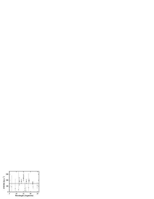
Figure 5: Half-width at half-maximum line widths derived from fitting Gaussian line-profile models to each individual line in the MEG first-order spectrum. The strongest, well behaved, isolated lines are indicated with darker symbols. The lower signal-to-noise, blended, or otherwise less reliable lines are shown in gray. 68% confidence limit error bars are shown for all the lines. The weighted mean HWHM velocity for all the lines is indicated by the dashed horizontal line, while the HWHM that corresponds to the turbulent velocity derived from the global spectral fit is indicated by the dotted horizontal line (recall that $v_{\mathrm{turb}}=180$ km s^-1 corresponds to a half width at half maximum of 150 km s^-1).

Figure 6: The C iv resonance doublet from several coadded archived IUE observations. A velocity scale (km s^-1) in the frame of the star is shown above the data. These lines show the characteristic blue-shifted absorption that is expected from a stellar wind, but the lines are not only weak compared to theoretical expectations but also much less wind broadened.

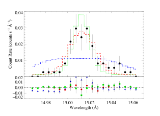
Figure 7: The Fe  xvii line at 15.014 Å with three different wind profile models. The red, dashed line is a constant-velocity wind model with $v_{\infty}=280$ km s^-1 (the best-fit value for a constant outflow velocity, which produces emission lines with $v_{\mathrm{hwhm}}\approx 150$ km s^-1). The model with $v_{\infty}=2000$ km s^-1, $\beta=1$, and $R_{\rm min}=1.5$ $\rm R_{\ast}$ is represented by the blue, dot-dash line. An infinitely narrow model is shown as the green, dotted line. The residuals for each model fit are shown in the lower panel, as red circles for the global best-fit, modestly broadened ($v_{\infty}=280$ km s^-1) model, green squares for the narrow profile model, and blue triangles for the broad wind model. The wind model with the higher velocity ($v_{\infty}=2000$ km s^-1) clearly does not provide a good fit, while the narrower constant velocity ($v_{\infty}=280$ km s^-1) wind model does. And while the very narrow model cannot be absolutely ruled out, the $v_{\infty}=280$ km s^-1 model is preferred over it with a high degree of significance. All the models shown here have been convolved with the instrumental response function (rmf) and multiplied by the wavelength-dependent effective area (garf).

However, although the theoretical expectation is for a fast wind with a terminal velocity of roughly 2000 km s^-1, the UV wind line profiles observed with IUE tell a different story. The UV line with the strongest wind signature is the C iv doublet at 1548,1551 Å, which shows a blue edge velocity of only 420 km s^-1 (Prinja, 1989). We show this line in Fig. 6. The Si  iii line shows no wind broadening and the Si  iv line shows a slightly weaker wind signature than the C  iv feature. Certainly the terminal velocity of the wind could be significantly higher than this, with the outer wind density being too low to cause noticeable absorption at high velocities. However, because the empirical evidence from these UV wind features indicates that the terminal velocity of the wind may actually be quite low, we refit the strong lines in the MEG spectrum with the wind-profile model, but this time using a terminal velocity of 420 km s^-1. The fits were again statistically good, and for these models, the fitted values of $R_{\rm min}$ were generally between 1.3 $\rm R_{\ast}$ and 1.5 $\rm R_{\ast}$, which are much more reasonable values for the onset radius of wind-shock emission.

We also considered a constant-velocity model ($\beta=0$), where the X-rays perhaps are produced in some sort of termination shock. For these fits, $R_{\rm min}$ hardly affects the line width, so we fixed it at 1.5 $\rm R_{\ast}$ and let the (constant) terminal velocity, $v_{\infty}$, be a free parameter. For the seven lines or line complexes with high enough signal-to-noise to make this fitting meaningful, we found best-fit velocities between 270 km s^-1 and 300 km s^-1 for five of them, with one having a best-fit value lower than this range and one line having a best-fit value higher than this range. The average wind velocity for these seven lines is $v_{\infty}=280$ km s^-1. All in all, the emission line widths are consistent with a constant-velocity outflow of $280$ km s^-1, and are inconsistent with a wind-shock origin in a wind with a terminal velocity of 2000 km s^-1. The lines are narrower than would be expected even for a wind with a terminal velocity not much greater than the observed C  iv blue edge velocity, $v=420$ km s^-1 (based on our $\beta=1$ fits as well as the $\beta=0$ fits). The X-ray emitting plasma must be moving significantly slower than the bulk wind. In Fig. 7 we show the best-fit constant velocity model ($v_{\infty}=280$ km s^-1) superimposed on the Fe  xvii line at 15.014 Å, along with the higher velocity model based on the theoretically expected terminal velocity, which clearly does not fit the data well. We also compare the best-fit wind-profile model to a completely narrow profile in this figure. The modestly wind-broadened profile that provides the best fit is preferred over the narrow profile at the 99% confidence level, based on the C statistic values of the respective fits (Numerical Recipes, Ch. 14; Press et al. (1982)).

4.1.3 Helium-like forbidden-to-intercombination line ratios

The final spectral diagnostic we employ is the UV-sensitive forbidden-to-intercombination line ratio of helium-like ions. These two transitions to the ground-state have vastly different lifetimes, so photoexcitation out of the $1{\rm s}2{\rm s}~{}^{3}{\rm S}_{1}$ state, which is the upper level of the forbidden line, to the $1{\rm s}2{\rm p}~{}^{3}{\rm P}_{1,2}$ state, which is the upper level of the intercombination line, can decrease the forbidden-to-intercombination line ratio, ${\mathcal{R}}\equiv f/i$. Because the photoexcitation rate depends on the local UV mean intensity, the $f/i$ ratio is a diagnostic of the distance of the X-ray emitting plasma from the photosphere. This diagnostic has been applied to many of the hot stars that have Chandra grating spectra, and typically shows a source location of at least half a stellar radius above the photosphere. Recently, Leutenegger et al. (2006) have shown that the $f/i$ ratios from a spatially distributed X-ray emitting plasma can be accounted for self-consistently with the line profile shapes in four O stars, providing a unified picture of wind-shock X-ray emission on O stars.

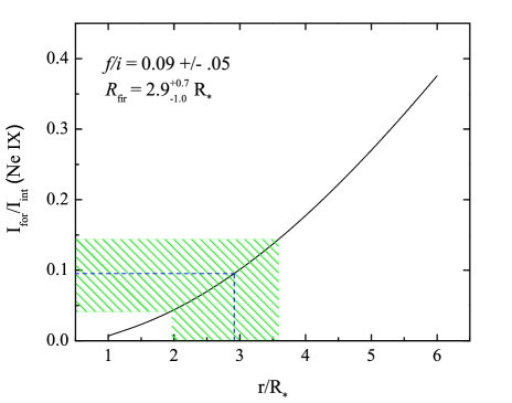
Figure 8: The Ne  ix resonance-intercombination-forbidden complex in the co-added MEG data, with the best-fit three-Gaussian model overplotted (top). The constraints on the measured $f/i$ ratio ($0.09\pm.05$), from the fit shown in the top panel, are indicated by the cross-hatched area’s intersection with the y-axis (bottom). The solid black curve is the model for the line ratio, as a function of radius. The cross-hatched region’s intersection with the model defines the 68% confidence limit on $r/\rm R_{\ast}$ of (1.9:3.6). The dashed line represents the best-fit value, $f/i=0.09$, and the corresponding $R_{\rm fir}=2.9$ $\rm R_{\ast}$.

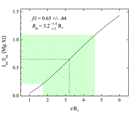
Figure 9: The Mg  xi resonance-intercombination-forbidden complex in the co-added MEG data, with the best-fit wind-profile models overplotted (top). The constraints on the formation radius, $R_{\rm fir}$, are shown in the bottom panel.

The lower-Z species like oxygen do not provide any meaningful constraints, as is the case for O stars, and there are not enough counts in the Si  xiii complex to put any meaningful constraints on the source location. Only the Ne  ix and Mg  xi complexes provide useful constraints. For both Ne  ix and Mg  xi we find $R_{\rm fir}\approx 3\pm 1\rm R_{\ast}$. Of course, the line-emitting plasma is actually distributed in the wind, and so we also fit the same modified Owocki & Cohen (2001) wind profile model that Leutenegger et al. (2006) used to fit a distributed X-ray source model to the He-like complexes, accounting simultaneously for line ratio variations and wind-broadened line profiles. With the wind velocity law and ${\mathcal{G}}\equiv\frac{f+i}{r}$ as free parameters, strong constraints could not be put on the models. Typically, these distributed models of $\mathit{f}/i$ gave onset radii, $R_{\rm min}$, that were quite a bit lower than $R_{\rm fir}$. This is not surprising, because a distributed model will inevitably have some emission closer to the star than $R_{\rm fir}$ to compensate for some emission arising at larger radii. We list the results of such a wind-profile fit to the He-like complexes in Tab. 5 along with the $R_{\rm fir}$ values. The two helium-like complexes and the best-fit models are shown in Figs. 8 and 9, along with the modeling of the $f/i$ ratios and the characteristic formation radii, $R_{\rm fir}$. We note that the data rule out plasma right at the photosphere only at the 68% confidence level.

We derive a single characteristic radius of formation, $R_{\rm fir}$, for each complex by calculating the dependence of the $f/i$ ratio on the distance from the photosphere, using a TLUSTY model atmosphere (Lanz & Hubeny, 2007). We used the formalism of Blumenthal et al. (1972), equation (1c), ignoring collisional excitation out of the ${}^{3}{\rm S}_{1}$ level, and explicitly expressing the dependence on the dilution factor, and thus the radius, as in equation (3) in Leutenegger et al. (2006). The measurement of $f/i$ from the data can then be used to constrain the characteristic formation radius, $R_{\rm fir}$.

4.2 Time Variability Analysis

We first examined the Chandra data for overall, stochastic variability. Both a K-S test applied to the unbinned photon arrival times and a ${\chi}^{2}$ fitting of a constant source model to the binned light curve showed no evidence for variability in the combined zeroth order and first order spectra. This is to be expected from wind-shock X-rays, which generally show no significant variability. This is usually interpreted as evidence that the X-ray emitting plasma is distributed over numerous spatial regions in the stellar wind (Cohen et al., 1997). Separate tests of the hard ($h\nu>1$ keV) and soft ($h\nu<1$ keV) counts showed no evidence for variability in the soft data, but some evidence for variability (K-S statistic implies 98% significance) in the hard data.

Because $\beta$ Cru is a $\beta$ Cephei variable, we also tested the data for periodic variability. Both the changes in the star’s effective temperature with phase and the possible effects of wave leakage of the pulsations into the stellar wind could cause the X-ray emission, if it arises in wind shocks, to show a dependence on the pulsation phase (Owocki & Cranmer, 2002). Our Chandra observation covers about four pulsation periods. To test for periodic variability, we used a variant of the K-S test, the Kuiper test (Paltani, 2004), which is also applied to unbinned photon arrival times. To test the significance of a given periodicity, we converted the photon arrival times to phase and formed a cumulative distribution of arrival phases from the events table. We then calculated the Kuiper statistic and its significance for that particular period. By repeating this process for a grid of test periods, we identified significant periodicities in the data.

Figure 10: Rejection probability (significance level increasing downward) of assumed period, according to the Kuiper statistic. The five known optical pulsation periods (Aerts et al., 1998; Cuypers et al., 2002) are indicated by the vertical lines. The primary pulsation period is the third of these.

Figure 11: The light curve of the hard counts in the zeroth and first order spectra of the primary, along with the best-fit sinusoidal model.

When we applied this procedure to all the zeroth-order and first-order counts we did not find any significant periodicities. However, applying it only to the hard counts produced a significant peak near the primary and tertiary optical pulsation periods ($f_{1}$ and $f_{3}$) of 4.588 hours and 4.386 hours (Aerts et al., 1998), as shown in Fig. 10. This peak is significant at the 99.95% level. It is relatively broad as the data set covers only about four cycles of the pulsation, so it is consistent with both pulsation modes, but not with the secondary ($f_{2}$) mode (Aerts et al., 1998). No significant periods are found in the soft bandpass, despite the higher signal-to-noise there. To quantify the level of periodic variability we found in the hard counts, we made a binned light curve from these counts and fit a sine wave with a period of 4.588 hours, leaving only the phase and the amplitude as free parameters. We find a best-fit amplitude of 18%. We show the light curve and this fit in Fig. 11 and note that there appears to be some additional variability signal beyond the strictly periodic component. We also note that there is a phase shift of about a quarter period ($\Delta\phi=0.27\pm.04$) between the times of maximum X-ray and optical light, with the X-rays lagging behind the optical variability. To make this assessment, we compared the time of maximum X-ray light from the sinusoidal fitting shown in Fig. 11 to the time of maximum optical light in the WIRE data, based on just the primary pulsation mode (Cuypers 2007, private communication). We note that $\phi=0.25$ corresponds to the maximum blue shift in the radial velocity variability of $\beta$ Cephei stars (Mathias et al., 1992).

5 Analysis of the companion

We subjected the newly discovered companion to most of the same analyses we have applied to $\beta$ Cru, as described in the previous section. The exceptions are the wind-profile fitting, which is not relevant for the unresolved lines in the companion’s spectrum, and the tests for periodic variability, since none is expected.

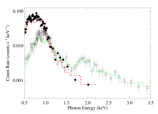
Figure 12: The zeroth order spectrum of the companion (open squares) is shown along with that of $\beta$ Cru (filled circles). The companion’s spectrum is significantly harder, and is well-fit by a two-temperature thermal model with component temperatures several times higher than those found for $\beta$ Cru. The best-fit models – to the combined zeroth order and grating spectra – are shown as the dashed ($\beta$ Cru) and dotted (companion) lines.

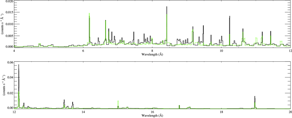
Figure 13: The best-fit two-temperature, variable abundance thermal spectral (APEC) model (green, dotted line), superimposed on the adaptively smoothed co-added MEG first-order spectrum of the companion (black, solid line).

Our working hypothesis is that the X-ray bright companion is a low-mass pre-main-sequence star, similar to those found in the ROSAT pointing (Park & Finley, 1996; Feigelson & Lawson, 1997; Alcalá et al., 2002). In the following two subsections, we marshal evidence from the spectral and time-variability properties to address this hypothesis.

5.1 Spectral Analysis

The spectrum of the companion is significantly harder than that of $\beta$ Cru. This can be seen in both the zeroth-order spectrum (see Fig. 12 and Fig. 1) and the dispersed spectrum (see Fig. 13). The dispersed spectrum has quite poor signal-to-noise, as the hardness leads to fewer counts per unit energy flux.

We fit a two-temperature optically thin coronal equilibrium spectral model to the zeroth order spectrum of the companion. As we did for the primary, we compared the best-fit model’s predictions to the MEG spectrum and found good agreement. This source is significantly harder than $\beta$ Cru, as indicated by the model fit, which has component temperatures of 6.2 and 24 million K. The emission measures of the two components are $1.8\times 10^{52}$ cm^-3 and $4.2\times 10^{52}$ cm^-3, respectively, yielding an X-ray flux of $5.71\pm.06\times 10^{-13}$ ergs s^-1 cm^-2, corrected for ISM absorption using the same column density that we used for the analysis of the spectrum of $\beta$ Cru. This flux implies $L_{\rm x}=8.0\times 10^{29}$ ergs s^-1. No significant constraints can be put on the abundances of the X-ray emitting plasma from fitting the Chandra data. This best-fit two-temperature APEC model is shown superimposed on the adaptively smoothed, coadded MEG spectrum in Fig. 13 (it is also shown, as the dotted histogram, in Fig. 12). These MEG data are much noisier than those from $\beta$ Cru, but the overall fit is reasonable, and the stronger continuum, indicative of higher temperature thermal emission is quite well fit. We note that only three of the line complexes have even a dozen counts in this spectrum.

Unlike $\beta$ Cru, the companion has lines that are narrow – unresolved at the resolution limit of the HETGS. This, and the hardness of the spectrum, indicates that the companion is consistent with being an active low-mass main-sequence or pre-main-sequence star.

The $f/i$ ratios that provided information about the UV mean intensity and thus the source distance from the photosphere in the case of $\beta$ Cru can be used in coronal sources as a density diagnostic. The depopulation of the upper level of the forbidden line will be driven by collisions, rather than photoexcitation, in the case of cooler stars. Some classical T Tauri stars (cTTSs) have shown anomalously low $f/i$ ratios compared to main sequence stars and even weak-line T Tauri stars (wTTSs) (Kastner et al., 2002; Schmitt et al., 2005). The best constraint in the companion’s spectrum is provided by Ne  ix, which has $f/i=2.2\pm 1.1$. This value is consistent with the low-density limit of $f/i=3.0$ (Porquet & Dubau, 2000), which is typically seen in wTTSs and active main sequence stars but is sometimes altered in cTTSs. Using the calculations in Porquet & Dubau (2000), we can place an upper limit on the electron density of $n_{\rm e}\approx 10^{12}$ cm^-3, based on the $1\sigma$ lower limit of the $f/i$ ratio.

5.2 Time Variability Analysis

Figure 14: The binned light curve of the companion, including all zeroth- and first-order counts.

Figure 15: The hardness ratio as a function of time, defined as $HR\equiv\frac{CR{\mathrm{(>1keV)}}-CR{\mathrm{(<1keV)}}}{CR{\mathrm{(>1keV)}}+CR{\mathrm{(<1keV)}}}$, where $CR$ denotes the count rate in the combined zeroth order and first order (MEG) data, over the indicated photon energy ranges. We fit a linear function to the data, and find $\chi^{2}=25$ for 24 degrees of freedom for a constant model (slope of zero), so a constant source model cannot be rejected outright. However, the best-fit slope of $-1.9\times 10^{-6}$ cts s^-2 (solid line) gives $\chi^{2}=20$, for 23 degrees of freedom, which is a statistically significant improvement over the constant model.

The companion is clearly much more variable than is $\beta$ Cru. The K-S test of the unbinned photon arrival times compared to a constant source model shows significant variability in all energy bands, though the significance is higher in the hard X-rays ($h\nu>1$ keV). The binned light curve also shows highly significant variability, again with the null hypothesis of a constant source rejected for the overall data, and both the soft and hard counts, separately. An overall decrease in the count rate is clearly seen as the observation progressed (Fig. 14).

The short rise followed by a steady decline of nearly 50% in the X-ray count rate over the remainder of the observation is qualitatively consistent with flare activity seen in late-type PMS stars (Favata et al., 2005), although the rise is not as rapid as would be expected for a single, large flare. We examined the spectral evolution of the companion during this decay, and there is mild evidence for a softening of the spectrum at late times, but not the dramatic spectral evolution expected from a cooling magnetic loop after a flare. For example, the hardness ratio (the difference between the count rate above 1 keV and below 1 keV, normalized by the total count rate) is shown in Fig. 15. There is a mild preference for a negative slope over a constant hardness ratio (significant at the 95% level), but with the data as noisy as they are, a constant hardness ratio cannot be definitively ruled out.

6 Discussion and Conclusions

Although it is very hot and luminous, $\beta$ Cru has a Chandra spectrum that looks qualitatively quite different from those of O stars, with their significantly Doppler broadened X-ray emission lines. Specifically, the emission lines of $\beta$ Cru are quite narrow, although they are resolved in the MEG, with half-widths of $\sim 150$ km s^-1. These relatively narrow lines are incompatible with the wind-shock scenario that applies to O stars if the wind of $\beta$ Cru has a terminal velocity close to the expected value of $v_{\infty}\approx 2000$ km s^-1. They are, however, consistent with a spherically symmetric outflow with a constant velocity of $v_{\infty}=280$ km s^-1.

If the wind terminal velocity is significantly less than 2000 km s^-1 – perhaps just a few hundred km s^-1 above the $420$ km s^-1 maximum absorption velocity shown by the strongest of the observed UV wind lines – a wind-shock origin of the X-ray emission is possible, but still difficult to explain physically. One wind-shock scenario that we have considered relies on the fact that the low-density wind of $\beta$ Cru should take a long time to cool once it is shock heated. If a large fraction of the accelerating wind flow passes through a relatively strong shock front at $r\approx 1.5$ $\rm R_{\ast}$, where the pre-shock wind velocity may be somewhat less than 1000 km s^-1, it could be decelerated to just a few 100 km s^-1, explaining the rather narrow X-ray emission lines. Similar onset radii are seen observationally in O stars (Kramer et al., 2003; Cohen et al., 2006; Leutenegger et al., 2006). The hottest plasma component from the global thermal spectral modeling requires a shock jump velocity of roughly 700 km s^-1, with the dominant cooler component requiring a shock jump velocity of roughly 400 km s^-1.

The $\mathit{f}/i$ ratios of Ne  ix and Mg  xi indicate that the hot plasma is either several stellar radii from the photosphere or distributed throughout the wind starting at several tenths of a stellar radius. This is broadly consistent with this scenario of an X-ray emitting outer wind. The lack of overall X-ray variability would also be broadly consistent with this quasi-steady-state wind-shock scenario. And the periodic variability seen in the hard X-rays could indicate that the shock front conditions are responding to the stellar pulsations, while the lack of soft X-ray variability would be explained if the softer X-rays come from cooling post-shock plasma in which the variability signal has been washed out.

The overall level of X-ray emission is quite high given the modest wind density, which is a problem that has been long-recognized in early B stars (Cohen et al., 1997). A large fraction of the wind is required to explain the X-ray emission. Elaborating on the scenario of a shock-heated and inefficiently cooled outer wind, we can crudely relate the observed X-ray emission measure to the uncertain mass-loss rate.

Assuming a spherically symmetric wind in which the X-rays arise in a constant-velocity post-shock region that begins at a location, $R_{0}$, somewhat above the photosphere; say $R_{0}\approx 1.5$ (in units of $\rm R_{\ast}$), we can calculate the emission measure available for X-ray production from

$$\mathcal{E}M\equiv\int n_{\rm e}n_{\rm H}dV=\int^{\infty}_{R_{0}}n_{\rm e}n_{\rm H}4\pi r^{2}dr.$$

Again assuming spherical symmetry and a smooth flow with a constant velocity for $r>R_{0}$, we have

$$\mathcal{E}M=1.3\times 10^{54}\frac{\dot{M}_{-9}^{2}}{R_{0}v_{\rm 100}^{2}}~{}~{}~{}{\rm(cm^{-3})}$$

for the emission measure of the entire wind above $r=R_{0}$, where $\dot{M}_{-9}$ is the mass-loss rate in units of $10^{-9}\mathrm{M_{\sun}~{}{\mathrm{y}r^{-1}}}$ and $v_{\rm 100}$ is the wind velocity in units of $100$ km s^-1. Equating this estimate of the available emission measure to that which is actually observed in the data, $3.5\times 10^{53}$ cm^-3, we get

$$\dot{M}_{-9}=\sqrt{\frac{\mathcal{E}M}{1.3\times 10^{54}}R_{0}v_{\rm 100}^{2}}\approx 1$$

for $R_{0}\approx 1.5$ and $v=280$ km s^-1 ($v_{\rm 100}=2.8$), which is the velocity obtained from fitting the line widths in the MEG spectrum. Thus a mass-loss rate of order $10^{-9}\mathrm{M_{\sun}~{}{\mathrm{y}r^{-1}}}$ is consistent with the observed X-ray emission measure. This type of simple analysis relating the observed X-ray emission measure in early B stars to their mass-loss rate in the context of shock heating and inefficient radiative cooling in the outer wind was applied to ROSAT observations of the early B giants $\epsilon$ and $\beta$ CMa by Drew et al. (1994), who, like we have here, found lower mass-loss rates than expected from theory. A downward revision in the mass-loss rates of early B stars might not be surprising given recent work indicating that the mass-loss rates of O stars have been overestimated (Bouret et al., 2005; Fullerton et al., 2006; Cohen et al., 2007).

Given the estimated mass-loss rate of $\dot{M}\approx 10^{-9}$ $\mathrm{M_{\sun}~{}{\mathrm{y}r^{-1}}}$ for $\beta$ Cru, we can assess the cooling time, or cooling length, of the purported wind shocks. A crude estimate of the cooling time and length of shock-heated wind material can be made by comparing the thermal energy content of the post-shock plasma,

$$E_{\mathrm{th}}=\frac{3}{2}n{\rm k}T\approx 0.1~{}~{}~{}~{}{\rm(ergs~{}cm^{-3})}$$

to the radiative cooling rate,

$$\frac{dE}{dt}=n^{2}\Lambda\approx 5\times 10^{-7}~{}~{}~{}~{}{\rm(ergs~{}s^{-1}~{}cm^{-3})}.$$

These numbers come from taking expected values of the wind density based on the assumptions of spherical symmetry of the wind and a constant outflow velocity,

$$n=6\times 10^{8}\frac{\dot{M}_{-9}}{R^{2}v_{\rm 100}}~{}~{}~{}~{}{\rm(cm^{-3}),}$$

where $R$ is the radial location in units of stellar radii. Using $v_{\rm 100}=2.8$ and $\dot{M}_{-9}=1$, the density is just $n\approx 10^{8}$ cm^-3 at $R=1.5$. We use temperatures of $T=2.5$ and $6.5\times 10^{6}$ K, given by the spectral fitting discussed in §4.1, assuming that some of the softer thermal component is produced directly by shock heating (rather than by radiative cooling of hotter plasma) since the emission measure of the hot component is so small. We take the integrated line emissivity to be $\Lambda\approx 5\times 10^{-23}$ ergs s^-1 cm³ for a plasma of several million K (Benjamin et al., 2001). The characteristic cooling time thus derived,

$$t_{\mathrm{cool}}=\frac{3{\rm k}T}{2n\Lambda}\approx 1~{}{\mathrm{to}}~{}2\times 10^{5}~{}~{}~{}~{}{\rm(s),}$$

is many times longer than the characteristic flow time,

$$t_{\mathrm{flow}}\equiv\frac{r}{v}\approx\frac{\rm R_{\ast}}{v}\approx 2\times 10^{4}~{}~{}~{}~{}{\rm(s).}$$

Thus, material shock heated to several million degrees at half a stellar radius above the surface will essentially never cool back down to the ambient wind temperature by radiative cooling, motivating the picture we have presented of a wind with an inner, cool acceleration zone and a quasi-steady-state outer region that is hot, ionized, X-ray emitting, and moving at a more-or-less constant velocity (because it is too highly ionized to be effectively radiatively driven).

Although the scenario we have outlined above is phenomenologically plausible, there are several significant problems with it. First of all, the behavior of wind shocks produced by the line-driving instability is not generally as we have described here. Such shocks tend to propagate outward at an appreciable fraction of the ambient wind velocity (Owocki et al., 1988; Feldmeier et al., 1997). Whereas the scenario we have outlined involves a strong shock that is nearly stationary in the frame of the star, as one would get from running the wind flow into a wall. There is, however, no wall for the wind to run into. It is conceivable that a given shock front forms near $r=1.5$ $\rm R_{\ast}$ and propagates outward, with another shock forming behind it (upstream) at roughly the same radius, so that the ensemble of shocks is close to steady state. However, the narrow observed X-ray lines severely limit the velocity of the shock front, as the post-shock velocity in the star’s frame must be greater the shock front’s velocity. Yet the observed lines are consistent with a post-shock flow of only $v=280$ km s^-1. A related, second, problem with the scenario is that the shocks required to heat the plasma to $T\approx 2.5$ to $6.5\times 10^{6}$ K are relatively strong for a weak wind. Smaller velocity dispersions are seen in statistical analyses of the LDI-induced structure in O star winds (Owocki & Runacres, 2002). Perhaps the purported wind shocks could be seeded by pulsations at the base of the wind. Seeding the instability at the base has been shown to lead to stronger shocks and more X-ray emission (Feldmeier et al., 1997), though the shocks still propagate relatively rapidly away from the star.

Another problem with this scenario is the very large X-ray production efficiency that is implied. Again, this general problem – that early B stars produce a lot of X-rays given their weak winds – has been known for quite some time. Quantifying it here, using the outer wind shock scenario presented above, and the mass-loss rate of $\dot{M}\approx 10^{-9}$ $\mathrm{M_{\sun}~{}{\mathrm{y}r^{-1}}}$ implied by this analysis, an appreciable fraction of the wind material is heated to X-ray emitting temperatures at any given time. And since the wind must be nearly completely decelerated when it passes through the shock front, a similar fraction of the available wind kinetic energy would go into heating the wind to $T\ga 10^{6}$ K. The self-excited LDI typically is much less efficient than this (Feldmeier et al., 1997).

If this scenario of a nearly completely shocked-heated outer wind with a low velocity is not likely, then what are the alternatives? As already stated, a more standard model of embedded wind shocks formed by the LDI and outflowing with the wind cannot explain the very modest X-ray emission line widths nor the relatively large emission measures (or shock heating efficiency). However, a standard coronal-type scenario, as applied successfully to cool stars, cannot explain the data either. Coronal sources do not have emission lines that can be resolved in the Chandra HETGS. And the $\mathit{f}/i$ ratios would be lower than observed if the hot plasma were magnetically confined near the surface of the star. And of course, there is no reasonable expectation of a strong dynamo in OB stars. The relative softness and lack of variability would also seem to argue against an origin for the X-rays in a traditional corona at the base of the wind.

Perhaps magnetic fields are involved, but just not in the context of a dynamo and corona. Magnetic channeling of hot-star winds has been shown to efficiently produce X-rays and that X-ray emission has only modestly broad emission lines (Gagné et al., 2005). There is, however, no indication that $\beta$ Cru has a magnetic field. However, a field of only $B\approx 5$ G would be sufficiently strong to channel the low-density wind of $\beta$ Cru. The degree of magnetic confinement and channeling can be described by the parameter

$$\eta_{\ast}\equiv\frac{B^{2}R_{\ast}^{2}}{\dot{M}v_{\infty}},$$

where values of $\eta_{\ast}>1$ imply strong magnetic confinement and $B$ is the equatorial field strength for an assumed dipole field (ud-Doula & Owocki, 2002). We note that a stronger field has already been detected in another $\beta$ Cephei star, $\beta$ Cep itself (Donati et al., 2002), though attempts to detect a field on $\beta$ Cru have not yet been successful (Hubrig et al., 2006). The upper limits on the field strength are roughly an order of magnitude higher than what would be needed for significant confinement and channeling, though. We also note that the radius of the last closed loop scales as $\eta_{\ast}^{0.5}$ (ud-Doula & Owocki, 2002), so a field of 50 G – still undetectable – would lead to a magnetosphere with closed field lines out to 3 $\rm R_{\ast}$, consistent with the value found for $R_{\rm fir}$in §4.1.3.

In a more speculative scenario, it is possible that the material giving rise to the X-ray emission is near the base of the wind, and is falling back toward the star – a failed wind. This scenario has been invoked to explain the X-ray emission from $\tau$ Sco (B0.2 V) (Howk et al., 2000), which subsequently had a complex surface magnetic field detected on it (Donati et al., 2006). If material gets accelerated off the surface by radiation pressure, but after moving a distance off the surface finds that it can no longer be accelerated – perhaps because of the formation of optically thick clumps - those clumps may stall or even fall back toward the star and interact with the ambient wind, leading to shock heating of wind material and material on the surfaces of the clumps. The problems with this scenario include the ad hoc nature of the clump formation and wind fall-back (though this behavior is in fact seen in conjunction with magnetic channeling (ud-Doula & Owocki, 2002; Gagné et al., 2005)) and the $\mathit{f}/i$ ratios which indicate that the hot material is several stellar radii above the surface. Chandra observations of $\tau$ Sco do show $\mathit{f}/i$ ratios consistent with hot plasma significantly above the photosphere and they also show only modestly broadened X-ray emission lines, similar to what we see in $\beta$ Cru, although the spectrum of $\tau$ Sco is significantly harder (Cohen et al., 2003).

Finally, perhaps the physical characteristics of a wind with a slow, hot outer component that we described in our initial scenario is correct – that is what the $\mathit{f}/i$ ratios and the line widths are telling us – but the heating mechanism is not LDI-related wind shocks. Instead a more complete plasma treatment may be required to describe at least the outer wind, where the densities are below $10^{8}$ cm^-3. In such low density winds, the radiatively driven ions can decouple from the protons and rapidly accelerate, leading to frictional heating (Springmann & Pauldrach, 1992; Gayley & Owocki, 1994; Krtička & Kubát, 2001; Owocki & Puls, 2002). Heating to X-ray emitting temperatures is predicted to occur only at about spectral type B5 (Krtička & Kubát, 2001), but perhaps if the wind mass-loss rates of B stars are lower than anticipated significant frictional heating could occur in early B stars, like $\beta$ Cru.

We point out that the energy requirements for heating the low density ($n<10^{8}$ cm^-3) outer wind of $\beta$ Cru are not severe at all. The heating mechanism might even involve wave propagation if there is even a weak magnetic field on this star. And once significantly heated, such low density circumstellar matter will tend to remain hot, due to the inefficiency of radiative cooling (Owocki, 2004). In this sense, the hot plasma in the wind of $\beta$ Cru could be considered a corona, and though likely initiated by radiation pressure as described in CAK theory, the low-density, slow, far wind of $\beta$ Cru might even be driven by gas pressure gradients.

None of these scenarios of X-ray production on $\beta$ Cru are both physically natural and also in agreement with all the available data. Although, if a magnetic field were to be detected on $\beta$ Cru, then the magnetically channeled wind shock interpretation would be quite reasonable. However, we stress that the main characteristics that constrain any models that may be put forward are quite secure: the plasma temperature is several million degrees; the emission is not highly variable, except for the periodic hard X-ray variability; the X-ray emission lines are broadened but only modestly so; and the X-ray production efficiency (if the X-ray emission is related to the star’s wind) is rather high. Finally, we note that the periodic signal in the hard X-rays and its phasing with the radial velocity variability might be a clue to the X-ray production mechanism.

Put in the context of the empirical X-ray spectral properties of OB stars, the case of $\beta$ Cru may be extreme but it seems to lie at one end of a continuum of line-profile behavior in hot stars with radiation-driven stellar winds. The late-type O stars $\delta$ Ori (Miller et al., 2002) and $\sigma$ Ori A (Skinner et al., 2004, 2008) have lines that are broad, but not as broad as would be expected in the standard wind-shock scenario given their known wind properties. Perhaps there is a gradual transition from stars with X-ray emission lines consistent with their fast stellar winds, such as $\zeta$ Pup (Kahn et al., 2001; Cassinelli et al., 2001; Kramer et al., 2003) and $\zeta$ Ori (Cohen et al., 2006), through some late O stars with X-ray lines of intermediate width, to early B stars like $\beta$ Cru for which Chandra can barely resolve their lines.

The newly discovered companion to $\beta$ Cru is most likely a low-mass pre-main-sequence star, similar to the post T Tauri stars found in the ROSAT data (Park & Finley, 1996; Alcalá et al., 2002). It has a hard, thermal spectrum as PMS stars do, and shows significant variability, again, as PMS stars do (Favata et al., 2005). The age of $\beta$ Cru is less than the pre-main-sequence lifetimes of most low-mass stars. Lindroos (1986) identified a few dozen B stars with likely PMS companions. If this newly discovered companion indeed is a PMS star, then $\beta$ Cru would be a Lindroos binary. As such, it would be useful for testing evolutionary models if an optical spectrum of the companion can be obtained. It would be especially helpful if enough information about the mid-B spectroscopic companion (which is supposed to still be on the main sequence (Aerts et al., 1998)) can also be obtained. There are systematic age differences as a function of spectral type in the LCC which seem to reflect problems with models (Preibisch & Mamajek, 2007), and the analysis of the three coeval stars in the $\beta$ Cru system could provide important constraints on the evolutionary models.

Given the companion’s X-ray luminosity of nearly $10^{30}$ ergs s^-1 cm^-2 at the assumed distance of 108 pc, even a G star somewhat above the main sequence would have a $f_{X}/f_{V}$ ratio consistent with those seen in PMS stars. The nearby K and M post-T Tauri stars detected in the ROSAT pointing are typically $m_{\mathrm{v}}\approx 13$ and have $f_{X}/f_{V}\approx 10^{-2}$ (Park & Finley, 1996). If the companion has a similar X-ray-to-V-magnitude flux ratio, then it is a $12^{th}$ magnitude PMS K star. If the magnitude difference between $\beta$ Cru and this newly discovered companion is roughly 11, then at a separation of 4″ and with the primary being so bright, detecting it with a ground-based optical or IR telescope will be a challenge, though such data would obviously be very useful for confirming its PMS status and characterizing its properties. Any accretion disk it might have would be significantly irradiated by UV light from the primary. Finally, given a projected separation of 430 AU, the companion should have an orbital period (around $\beta$ Cru and its spectroscopic companion) of at least 1000 years.

References

- Abbott (1982) Abbott D.C., 1982, ApJ, 259, 282
- Aerts et al. (1998) Aerts C., De Cat P., Cuypers J., Becker S.R., Mathias P., De Mey K., Gillet D., Waelkens C., 1998, A&A, 329, 137
- Alcalá et al. (2002) Alcalá J.M., Covino E., Melo C., Sterzik M.F., 2002, A&A, 384, 521
- Anders & Grevesse (1989) Anders E., Grevesse N., 1989, Geochimica et Cosmochimica Acta, 53, 197
- Benjamin et al. (2001) Benjamin R.A., Benson B.A., Cox D.P., 2001, ApJ, 554, L225
- Blaauw (1946) Blaauw A., 1946, Publications of the Kapteyn Astronomical Laboratory Groningen, 52, 1
- Bertelli et al. (1994) Bertelli G., Bressan A., Chiosi C., Fagotto F., Nasi E., 1994, A&AS, 106, 275
- Blumenthal et al. (1972) Blumenthal G.R., Drake G.W.F., Tucker W.H., 1972, ApJ, 172, 205
- Bouret et al. (2005) Bouret J.-C., Lanz T., Hillier D.J., 2005, A&A, 438, 301
- Canizares et al. (2005) Canizares C.R., et al., 2005, PASP, 117, 1144
- Cash (1979) Cash W., 1979, ApJ, 228, 939
- Cassinelli et al. (2001) Cassinelli J.P., Miller N.A., Waldron W.L., MacFarlane J.J., Cohen D.H., 2001, ApJ, 554, L55
- Castor et al. (1975) Castor J.I., Abbott D.C., Klein R.I., 1975, ApJ, 195, 157
- CXC (2007) Chandra X-ray Center, Chandra Proposers’ Observatory Guide, version 10.0, 2007. Cambridge, CXC, cxc.harvard.edu/proposer/POG/pdf/MPOG.pdf
- Cohen et al. (1996) Cohen D.H., Cooper R.G., MacFarlane J.J, Owocki S.P., Cassinelli J.P., Wang P., 1996, ApJ, 460, 506
- Cohen et al. (1997) Cohen D.H., Cassinelli J.P., & MacFarlane J.J, 1997, ApJ, 487, 867
- Cohen et al. (2003) Cohen D.H., de Messières G.E., MacFarlane J.J., Miller N.A., Cassinelli J.P., Owocki S.P., Liedahl D.A., 2003, ApJ, 586, 495
- Cohen et al. (2006) Cohen D.H., Leutenegger M.A., Grizzard K.T., Reed C.L., Kramer R.H., Owocki S.P., 2006, MNRAS, 368, 1905
- Cohen et al. (2007) Cohen D.H., Leutenegger M.A., Townsend R.H.D., 2007, in Hamann W.-R.,Feldmeier A., Oskinova L., eds, Clumping in Hot Star Winds. Potsdam, Univ.–Verl., in press, arXiv:0712.1050v1
- Cuypers (1983) Cuypers J., 1983, A&A, 127, 186
- Cuypers et al. (2002) Cuypers J., Aerts C., Buzasi D., Catanzarite J., Conrow T., Laher R., 2002, A&A, 392, 599
- Davis (2001) Davis J.E., 2001, ApJ, 562, 575
- de Geus et al. (1989) de Geus E.J., de Zeeuw P.T., Lub J., 1989, A&A, 216, 44
- de Zeeuw et al. (1999) de Zeeuw P. T., Hoogerwerf R., de Bruijne J. H. J., Brown A. G. A., Blaauw A., 1999, AJ, 117, 354
- Donati et al. (2002) Donati J.-F., Wade G.A., Babel J., Henrichs H.F., de Jong J.A., Harries T.J., 2002, MNRAS, 326, 1265
- Donati et al. (2006) Donati J.-F., et al., 2006, MNRAS, 370, 629
- Drew et al. (1994) Drew J.E., Denby M., Hoare M.G., 1994, MNRAS, 266, 917
- Favata et al. (2005) Favata R., Flaccomio E., Reale F., Micela G., Sciortino S., Shang H., Stassun K.G., Feigelson E.D., 2005, ApJ, 160, 469
- Feigelson & Lawson (1997) Feigelson E.D, Lawson W.A., 1997, AJ, 113, 2130
- Feldmeier et al. (1997) Feldmeier A., Puls J., Pauldrach A.W.A., 1997, A&A, 322, 878
- Fruscione et al. (1994) Fruscione A., Hawkins I., Jelinsky P., Wiercigroch A., 1994, ApJ, 94, 127
- Fullerton et al. (2006) Fullerton A.W., Massa D.L., Prinja R.K., 2006, ApJ, 637, 1025
- Gagné et al. (2005) Gagné M., Oksala M., Cohen D.H., Tonnesen S.K., ud-Doula A., Owocki S.P., Townsend R.H.D., MacFarlane J.J., 2005, ApJ, 628, 986
- Gayley & Owocki (1994) Gayley K.G., Owocki S.P., 1994, ApJ, 434, 684
- Hale (1994) Hale A., 1994, A&A, 107, 306
- Hanbury Brown et al. (1974) Hanbury Brown R., Davis J., Allen L.R., 1974, MNRAS, 167, 121
- Heintz (1957) Heintz W., 1957, The Observatory, 77, 200
- Hillier et al. (1993) Hillier D.J., Kudritzki R.–P., Pauldrach A.W.A., Baade D., Cassinelli J.P., Puls J., Schmitt J.H.M.M., 1993, ApJ, 276, 117
- Hiltner et al. (1969) Hiltner W.A., Garrison R.F., Schild R.E., 1969, ApJ, 157, 313
- Hoogerwerf (2000) Hoogerwerf R., 2000, MNRAS, 313, 43
- Howk et al. (2000) Howk J.C., Cassinelli J.P., Bjorkman J.E., Lamers H.J.G.L.M., 2000, ApJ, 534, 348
- Hubrig et al. (2006) Hubrig S., Briquet M., Schöller M., De Cat P., Mathys G., Aerts C., 2006, MNRAS, 369, L61
- Kahn et al. (2001) Kahn S.M., Leutenegger M.A., Cottam J., Rauw G., Vreux J.–M., den Boggende A.J.F., Mewe R., Güdel M., 2001, A&A, 365, L312
- Kastner et al. (2002) Kastner J.H., Huenemoerder D.P., Schulz N.S., Canizares C.R., Weintraub D.A., 2002, ApJ, 567, 434
- Kramer et al. (2003) Kramer R.H., Cohen D.H., Owocki S.P., 2003, ApJ, 592, 532
- Krtička & Kubát (2001) Krtička J., Kubát J., 2001, A&A, 359, 983
- Kudritzki et al. (1989) Kudritzki R.P., Pauldrach A.W.A., Puls J., Abbott D.C., 1989, A&A, 219, 205
- Lanz & Hubeny (2007) Lanz T., Hubeny I., 2007, ApJ, 169, 83
- Leutenegger et al. (2006) Leutenegger M.A., Paerels F.B.S., Kahn S.M., Cohen D.H., 2006, ApJ, 650, 1096
- Lindroos (1985) Lindroos K.P., 1985, A&AS, 60, 183
- Lindroos (1986) Lindroos K.P., 1986, A&A, 156, 223
- Maiz Apellániz et al. (2008) Maiz Apellániz J., Alfaro E.J., Sota A., 2008, in Bresolin F., Crowther P., Puls J., eds, Massive Stars as Cosmic Engines. Cambridge University Press, in press
- Mamajek, Meyer, & Liebert (2002) Mamajek E. E., Meyer M. R., Liebert J., 2002, AJ, 124, 1670
- Marshall et al. (2004) Marshall H.L., Dewey D., Ishibashi K., 2004, SPIE, 5165, 457
- Mathias et al. (1992) Mathias P., Gillet D., Crowe R., 1992, A&A, 257, 681
- Miller et al. (2002) Miller N.A., Cassinelli J.P., Waldron W.L., MacFarlane J.J., Cohen D.H., 2002, ApJ, 577, 951
- Morrison & McCammon (1983) Morrison R., McCammon D., 1983, ApJ, 270, 119
- Niemczura & Daszynska-Daszkiewicz (2005) Niemczura E., Daszynska-Daszkiewicz J., 2005, A&A, 433, 659
- Owocki (2004) Owocki S.P., 2004, in Heydari-Malayeri M., Stee Ph., Zahn J.-P., eds, Evolution of Massive Stars, Mass Loss and Winds. EAS Publication Series, 13, 163
- Owocki et al. (1988) Owocki S.P., Castor J.I., Rybicki G.B., 1988, ApJ, 335, 914
- Owocki & Cohen (2001) Owocki S.P., Cohen D.H., 2001, ApJ, 559, 1108
- Owocki & Cranmer (2002) Owocki S.P., Cranmer S.R., 2002, in Aerts C., Bedding T. R., Christensen-Dalsgaard J., eds, I.A.U. Coll. 185. San Francisco, ASP, 259, 512
- Owocki & Puls (2002) Owocki S.P., Puls J., 2002, ApJ, 568, 965
- Owocki & Runacres (2002) Owocki S.P., Runacres M.C., 2002, A&A, 381, 1015
- Paltani (2004) Paltani S., 2004, A&A, 420, 789
- Park & Finley (1996) Park S., Finley J.P., 1996, AJ, 112, 693
- Perryman et al. (1997) Perryman M.A.C., et al., 1997, A&A, 323, L49
- Popper (1968) Popper D.M., 1968, ApJ, 151, L51
- Porquet & Dubau (2000) Porquet D.,Dubau J., 2000, A&AS, 143, 495
- Preibisch & Mamajek (2007) Preibisch T., Mamajek E., 2007, in B. Reipurth, ed, Handbook of Star Forming Regions Vol. II. The Southern Sky, in press
- Press et al. (1982) Press W.H., Flannery B.P., Teukolsky S.A., Vetterling W.T., 1982, Numerical Recipes, 2nd edition. Cambridge, Cambridge University Press, Ch. 14
- Prinja (1989) Prinja R.K., 1989, MNRAS, 241, 721
- Schmitt et al. (2005) Schmitt J.H.M.M., Robrade J., Ness J.-U., Favata F., Stelzer B., 2005, A&A, 432, L35
- Smith et al. (2001) Smith R.K, Brickhouse N.S., Liedahl D.A., Raymond J.C., 2001, ApJ, 556, L91
- Skinner et al. (2004) Skinner S.L., Cohen D.H., Gagné M., Owocki S.P., Townsend R.H.D., 2004, BAAS, 20510517S
- Skinner et al. (2008) Skinner S.L., Sokal K.R., Cohen D.H., Gagné M., Owocki S.P., Townsend R.H.D., 2008, in preparation
- Stankov & Handler (2005) Stankov A., Handler G., 2005, ApJ, 158, 193
- Springmann & Pauldrach (1992) Springmann U.W.E., Pauldrach A.W.A., 1992, A&A, 262, 515
- ud-Doula & Owocki (2002) ud-Doula A., Owocki S.P., 2002, ApJ, 576, 413
- Uesugi & Fukuda (1982) Uesugi A., Fukuda I., 1982, Catalogue of stellar rotational velocities (revised). Kyoto: University of Kyoto, Department of Astronomy
- van Leeuwen (2007a) van Leeuwen R., 2007a, A&A, 474, 653
- van Leeuwen (2007b) van Leeuwen R., 2007b, Hipparcos, the New Reduction of the Raw Data. Springer, Berlin
- Vink et al. (2000) Vink J. S., de Koter A., Lamers H.J.G.L.M., 2000, A&A, 362, 295
- Wolk (2002) Wolk S.J., 2002, Chandra Calibration Workshop. cxc.harvard.edu/ccw/proceedings/02_proc/
- Worley & Douglass (1997) Worley C.E., Douglass G.G., 1997, A&AS, 125, 523
- Zhekov & Palla (2007) Zhekov S. A., Palla F., 2007, MNRAS, 382, 1224